Predictability of the Large Relaxations in a Cellular Automaton Model

Abstract

A simple one-dimensional cellular automaton model with threshold dynamics is introduced. It is loaded at a uniform rate and unloaded by abrupt relaxations. The cumulative distribution of the size of the relaxations is analytically computed and behaves as a power law with an exponent equal to $-1$. This coincides with the phenomenological Gutenberg-Richter behavior observed in Seismology for the cumulative statistics of earthquakes at the regional or global scale. The key point of the model is the zero-load state of the system after the occurrence of any relaxation, no matter what its size. This leads to an equipartition of probability between all possible load configurations in the system during the successive loading cycles. Each cycle ends with the occurrence of the greatest –or characteristic– relaxation in the system. The duration of the cycles in the model is statistically distributed with a coefficient of variation ranging from 0.5 to 1. The predictability of the characteristic relaxations is evaluated by means of error diagrams.This model illustrates the value of taking into account the refractory periods to obtain a considerable gain in the quality of the predictions.

1 Introduction

The cellular automaton model presented here will be denoted, for brevity, as the C-Model (CM). It has analogies and differences with the so called Minimalist Model (MM) [1, 2] that will be emphasized in the next Sections. These types of cellular automaton models appeared in the context of the Self Organised Criticality (SOC) paradigm, introduced by Bak et al. [3, 4], which meant a very important new conceptual perspective to try to understand complexity in nature in general and in natural hazards, such as forest-fires, landslides and earthquakes, in particular. The flagship of SOC is the sand-pile model. It is a conservative cellular automaton where the size-frequency distribution of avalanches exhibits a power-law behaviour where the exponent corresponding to the non-cumulative distribution is around $-1$.

We will pay particular interest to studying two properties of the CM, namely the probability of occurrence of a relaxation of size $k$ for a system of size $N$, and the probability distribution for the time interval between successive characteristic relaxations, i.e. for the length of the loading cycles. This distribution will be called $P_{N}(n)$, where $n$ is the discrete time elapsed since the occurrence of the last characteristic relaxation. The mean and the variance of $P_{N}(n)$ will receive special consideration for the reasons that will be explained later.

For a better perspective of the results of this model we will refer to two important concepts coming from seismology. The best established law in regional seismicity is the Gutenberg-Richter relation between the magnitude of an earthquake and its frequency. This law is of the power-law type when magnitudes are expressed in terms of rupture areas

$$\dot{N}\propto S^{-b},$$ (1)

where $\dot{N}$ is the number of observed earthquakes, per time unit, with rupture area equal to or greater than $S$, and $b$ is the so-called $b$-value, which is a universal phenomenological parameter with a value close to unity [5]. Note that equation (1) represents a cumulative distribution. The corresponding non-cumulative distribution would also be a fractal law with an exponent equal to

$$-(b+1)\sim-2.$$ (2)

The interpretation of $b$ as a sort of universal critical exponent in nature exactly equal to $1$ has spurred theoreticians for years and many ideas, typically based on specific models and/or mechanisms, have been offered to explain both the power law behavior of (1) and the value of the $b$ parameter [6, 7, 8, 9, 10, 11]. Therefore, the Sand Pile model is not suitable for describing the observed Gutenberg-Richter Relation. But other SOC cellular automaton models for earthquakes, such as those introduced by Olami, Feder and Christensen [9] provided, within a certain limit of conservation, a correct order of magnitude for the $b$ parameter. For a review of SOC and earthquakes, see [12, 13].

Besides, it is important to bear in mind that the above mentioned Gutenberg-Richter law is a property of regional seismicity, appearing when one averages seismicity over big enough areas and long enough time intervals (e.g. [14]). For individual faults, the type of size-frequency relationship is different from the G-R law and consists of an approximate power-law distribution of small events (small compared with the maximum earthquake size that a fault can support, given its area), which occur between roughly quasi-periodic earthquakes of much larger size that rupture the entire fault. These large quasi-periodic earthquakes are termed “characteristic” [15], and the resulting size-frequency relationship is the Characteristic Earthquake distribution. It must be mentioned that the very concept of characteristic earthquake is under debate [16, 17].

Although the terminology that we use in this paper is often reminiscent of the seismological jargon, the CM could be applied to any entity where energy enters at a constant smooth rate and exits in the form of sudden relaxations with a very low efficiency because of dissipation.

The structure of the paper is as follows. In Section 2, the rules of the model are given together with a table and several figures of numerical results. Section 3 is devoted to some analytical deductions. In particular, using several properties of Markov chains, we compute the stationary probabilities of the configurations in the CM, the probability of occurrence of relaxations of any size, and some other properties of the loading cycle. Section 4 is devoted to the evaluation of the predictability of the large relaxations in this model. This is accomplished by using the so called error diagrams. A brief discussion and the conclusions are gathered in Section 5. In a final Appendix we explain some detailed calculations for the case $N=3$.

2 The C-Model: rules and some numerical results

The CM is a simple one-dimensional cellular automaton with threshold dynamics. Consider a one-dimensional array of length $N$. The ordered positions in the array will be labeled by an integer index $i$ varying from $1$ to $N$. This system is loaded by receiving individual particles in the various positions of the array, and unloaded by emitting groups of particles through the first position $i=1$, which are called relaxations or events. These two functions proceed using the following five rules:

1. The incoming particles arrive at the system at a constant rate. Thus the time interval between successive particles will be the basic time unit in the evolution of the system. In comparison with this time interval, the time taken by the relaxations is negligible.

2. All the $N$ positions have the same probability of receiving a new particle. When a position receives a particle we say that it is occupied.

3. The reception of a particle saturates a position, i.e. if a new particle comes to a position already occupied, that particle is dissipated.

4. The position $i=1$ is special. When a particle goes to the first position a relaxation occurs. Then if all successive positions from $i=1$ to $i=k$ are occupied and the position $k+1$ is empty, the effect of the relaxation is to unload all the levels from $i=1$ to $i=k$. Hence the size of the event is $k$. The maximum relaxation corresponds to $k=N$, which is called the characteristic relaxation of the system.

5. Besides, those positions that were occupied by particles but were not affected by the relaxation lose their particles so that the array is left completely empty.

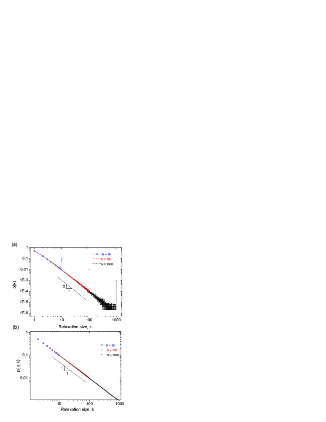
Figure 1: (a) Size-frequency plot for the relaxations in the CM; the three cases $N=10$, 100, and 1000 are superimposed. (b) cumulative magnitude-frequency plot. In both graphs a line of slope $-2$ (top) and $-1$ (bottom) has been added for visual comparison.

Table 1: Probability of occurrence of a relaxation of magnitude $k$ for a system size, $N$.

Size	N=2	N=3	N=4	N=10	N=100
k=1	0.50006	0.50003	0.50000	0.50009	0.49948
k=2	0.49994	0.16666	0.16652	0.16647	0.16667
k=3	-	0.33331	0.08333	0.08348	0.08359
k=4	-	-	0.25015	0.04994	0.05012
k=5	-	-	-	0.03339	0.03358
k=6	-	-	-	0.02370	0.02370
k=7	-	-	-	0.01785	0.01768
k=8	-	-	-	0.01396	0.01413
k=9	-	-	-	0.01108	0.01118
k=10	-	-	-	0.10002	0.00906
k=99	-	-	-	-	0.00009
k=100	-	-	-	-	0.00990

Thus in the CM, after any small relaxation, the system always restarts from the empty state, keeping no memory. The simplicity of these five rules makes it very appropriate for numerical simulations. The formalism and results of the Markov Chains can also be applied to this model. In contrast with the CM, in the MM [1], rule 5 did not exist. The fifth rule of this model could be representative of what occurs with the precipitation of a cloud. In the process of growth of the CCN (cloud condensation nuclei) by condensation, only those CCN that have been activated become cloud droplets and take part in the posterior processes of collision and coalescence, and therefore only they eventually contribute to the rain. The so-called haze droplets that were not activated evaporate.

Using these five rules and carrying out numerical simulations, we have obtained the results contained in Table 1 and in figures 1-4, and figures 6 and 7 later. From Table 1 and Fig. 1a we see that in the CM the value of $p_{k}(k<N)$ is an $N$-independent constant. This sort of scale invariance, which also appeared in the MM, can be justified by using the same arguments written in Ref. [1]. We also note that the non-cumulative size-frequency plot for the events in this model is of the Characteristic Earthquake type, as mentioned in the Introduction. In Fig. 1b, it is shown that, independently of $N$, the cumulative size-frequency plot for the relaxations in this model is a perfect power law with an exponent equal to $-1$. It is worth saying at this point that, as far as the authors know, there is no other model with this beautiful property. In the next Section, a probabilistic argument will be provided for this notable result.

Note that the non-cumulative distribution in Fig. 1a clearly shows the special character of the maximum magnitude relaxation, while the cumulative distribution hides this preponderance.

In Fig. 2, we show the probability distribution for the length of the cycles, $P_{N}(n)$, for $N=3$ (squares) and $N=10$ (circles). In both cases the distribution shows an initial refractory period (i.e., an interval of null probability of relaxation occurrence) of length equal to $N-1$, and a slow asymptotic decrease which will be reflected in the high variances of this model. In case $P_{3}(n)$, the results obtained by simulations are compared with the analytical result (continuous line) obtained in the Appendix.

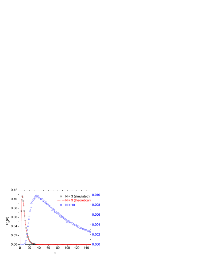
Figure 2: Probability distribution for the length of the cycles, $P_{N}(n)$, for $N=3$ (squares, left axis), and $N=10$ (circles, right axis). In the $N=3$ case the simulation result is compared with the analytical result (continuous line).

3 Stationary Probabilities in the CM, Spectrum of Earthquakes and other Analytic Properties

In the CM, for a system of size $N$, there are $N$ groups of configurations distinguished by their index of load occupation $\theta$,

$$\theta=0,1,2,\dots,N-1.$$ (3)

In each of these groups there are

$$\left({\begin{array}[]{*{20}c}N-1\\ \theta\\ \end{array}}\right)$$ (4)

different stationary configurations denoted by $\theta_{j}$, where the integer index $j$ runs in the range

$$1\leq j\leq\left({\begin{array}[]{*{20}c}N-1\\ \theta\\ \end{array}}\right).$$ (5)

As in any Markov chain of this type, if the Markov matrix is denoted by $\mathbf{M}$, then the stationary probabilities for each configuration are the components of the eigenvector of $\mathbf{M}^{T}$ corresponding to the eigenvalue $+1$. These components will be denoted by $\pi(\theta_{j})$. Their $j$-independent values are

$$\pi(\theta_{j})=\frac{1}{N}\frac{1}{\left({\begin{array}[]{*{20}c}N-1\\ \theta\\ \end{array}}\right)}.$$ (6)

Relations (6) are identified in a straightforward way because of the regularity of the Markov matrix $\mathbf{M}$ in this model (as an illustration, the case $N=3$ is worked out in detail in the Appendix). Thus, all the configurations that share the same $\theta$ have the same probability, and the sum of the probabilities of all of them is $1/N$. In other words, any load $\theta$ in this system has identical probability $1/N$, and the probability among all the possible configurations corresponding to a given $\theta$ is also equally distributed.

Using these results, let us compute first the fraction of particles that, on their way to a position in the array, find this position occupied and are therefore lost. This proportion will be called the reflectivity $\rho$ of the system:

$$\rho = \sum_{\theta_{j}}\pi(\theta_{j})\frac{\theta}{N}=\sum_{\theta}\left({\begin{array}[]{*{20}c}N-1\\ \theta\\ \end{array}}\right)\frac{1}{N}\frac{1}{\left({\begin{array}[]{*{20}c}N-1\\ \theta\\ \end{array}}\right)}\frac{\theta}{N}$$ (11)

$$= \frac{1}{N^{2}}\sum_{\theta=0}^{\theta=N-1}\theta=\frac{1}{N^{2}}\frac{N(N-1)}{2}=\frac{1}{2}\left(1-\frac{1}{N}\right).$$ (12)

Thus, for large $N$ nearly 50% of the particles are lost by reflection. This result is compared with the simulations in figure 3. We see there that the reflectivity (open and filled squares) increases with the system size, abruptly at the beginning and more slowly for bigger system sizes, reaching an asymptotic value of $\sim 0.5$ for big systems ($N\geq 200$). The smallest reflectivity is $\rho\sim 0.34$ for $N=3$.

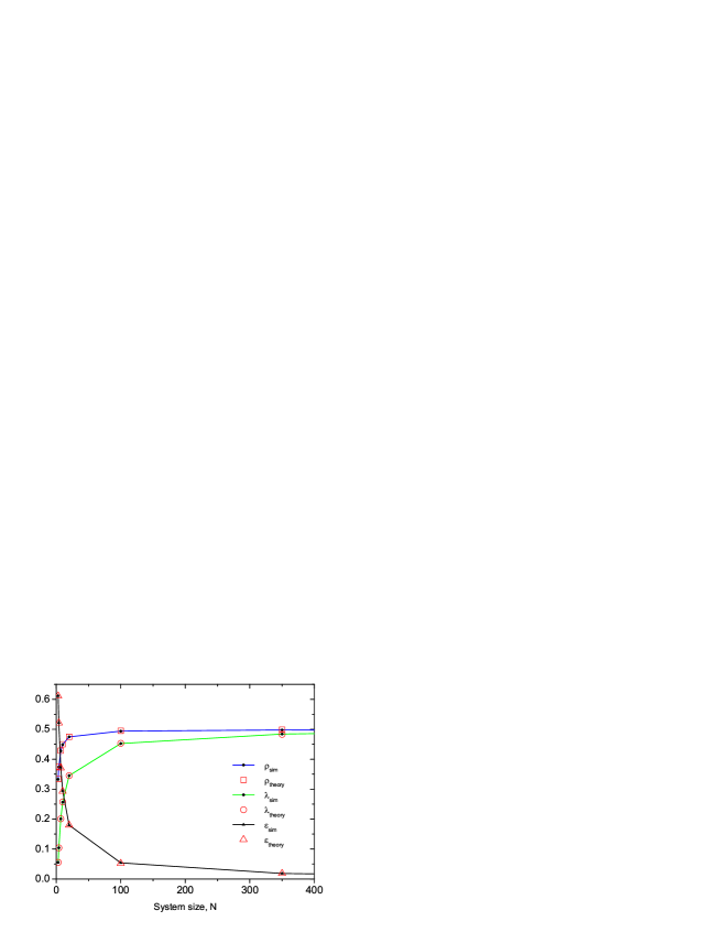
Figure 3: Reflectivity $\rho$, efficiency $\epsilon$, and fraction of lost particles during relaxations $\lambda$ as a function of $N$. For details, see Section 3.

A second analytical conclusion is the following. From Eq.(6), we know that in the case of maximum occupation, i.e., when there are $N-1$ particles in the system, its probability is

$$\pi(N-1)=\frac{1}{N},$$ (13)

therefore the probability that at any arbitrary time a characteristic event occurs is $1/N^{2}$ and, in consequence, the mean value of the time elapsed between two consecutive characteristic relaxations in this model is

$$<P_{N}(n)>=N^{2}.$$ (14)

This conclusion coincides with the numerical result presented in figure 4a, better seen in the inset where log-log scales have been used to appreciate the +2-slope trend of the mean. Note also how, for small system sizes, the mean is bigger than the standard deviation but that both of them tend to a common value as the system size increases. This can be better appreciated in figure 4b where the aperiodicity, i.e. the ratio of the standard deviation to the mean, is plotted. The minimum aperiodicity is 0.57 ($N=3$) and grows asymptotically to unity.

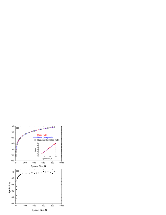
Figure 4: (a) Mean and standard deviation of $P_{N}(n)$ as a function of $N$; the inset shows the trend of the mean in log-log scales. MC stands for MonteCarlo results. (b) Aperiodicity versus $N$.

We also know that the mean time between two arbitrary consecutive relaxations in the model is $N$, and therefore we deduce that in this model, between two consecutive characteristic events, there are, on average, $N-1$ non-characteristic relaxations.

As mentioned above, a cycle is the time between two successive characteristic events. And each cycle is formed by a succession of several initial sub-cycles, marked by the occurrence of non characteristic events, and a final sub-cycle marked by the occurrence of the characteristic relaxation that ends the cycle. The calculation of the length of the final sub-cycle is straightforward. This time length is formed by the addition of two independent stages. The first stage, which starts from the state $\theta=0$ and ends when the system arrives to the state $\theta=N-1$, will be called the loading stage. The second, in which the system is completely loaded, ends when a particle hits the first site; this will be called the hitting stage. The length of the loading stage is the mean time taken to fill a box of $N-1$ cells by random assignments of the particles taking into account the reflection of particles by occupied cells [18]. The length of the hitting stage is the mean time of a geometric distribution with a hitting probability equal to $1/N$. Thus, we have

$$<n>_{fsc}=<n>_{l}+<n>_{h}=N(S-1)+N,$$ (15)

where $S$ is a function of $N$ defined as

$$S=\sum_{k=1}^{N}\frac{1}{k}.$$ (16)

For $N\geq 10$, $S$ is already well approximated by

$$\lim_{N\rightarrow\infty}S=C+\ln N+\frac{1}{2N}+\mathcal{O}\left(\frac{1}{N^{2}}\right),$$ (17)

where $C=0.577215\dots$ is Euler’s constant. Therefore, the asymptotic behavior of the duration of the final sub-cycle is of the form

$$\lim_{N\rightarrow\infty}<n>_{fsc}=N\ln N.$$ (18)

The variance of the time length of the final sub-cycle can also be analytically calculated.

Using numerical simulations, we have also seen in Section 2 that the CM provides a power-law relation, with $b=1$, for the cumulative size-frequency distribution of the relaxations. This power-law relation can be understood by a simple probabilistic argument. In the CM, after any relaxation, the grid contains no particles, i.e., all the positions of the system are empty. Therefore, to have in the next event a relaxation of size $\geq k$ $(1\leq k\leq N)$, it is necessary that the process of occupation of the lowest $k$ levels be in such a way that the first level ($i=1$) is the last one to be occupied. The question then is: What is the probability that $k$ identical sites be occupied with the condition that one of them be the last? As all of the sites are equivalent, the answer is

$$\frac{1}{k}.$$ (19)

Thus, for $1\leq k\leq N$,

$$p(\geq k)=\frac{1}{k}$$ (20)

independently of the size $N$ of the system.

Now, due to the fact that

$$p(k)=p(\geq k)-p(\geq k+1),$$ (21)

which can be applied for $1\leq k\leq N-1$ , we find that

$$p(k)=\frac{1}{k}-\frac{1}{k+1}=\frac{1}{k(k+1)}=\frac{1}{k^{2}(1+1/k)},$$

$$k\leq N-1.$$ (22)

For the limit case $k=N$, we apply expression (20) and obtain

$$p(k=N)=p(k\geq N)=\frac{1}{N}.$$ (23)

The verification of the adequate normalization of $p(k)$ is carried out as follows:

$$\sum_{k=1}^{N-1}p(k)+p(N) = \sum_{k=1}^{N-1}\left(\frac{1}{k}-\frac{1}{k+1}\right)+\frac{1}{N}$$ (24)

$$= 1-\frac{1}{N}+\frac{1}{N}=1.$$

Therefore, in the CM the cumulative spectrum of relaxation given in (20) constitutes a power law with an exponent $-1$. This coincides with the phenomenological Gutenberg - Richter exponent observed in seismology for the cumulative statistics at the regional or global scale. And according to this, in the CM the non-cumulative form of the size-frequency relation, as given in (3), is asymptotically a power law with an exponent equal to $-2$. These conclusions exactly reproduce the plots in figure 1. Relation (21) is the discrete derivation of (20); in the continuum it would correspond to

$$-\frac{d}{dx}\frac{1}{x}=\frac{1}{x^{2}}.$$ (25)

With respect to the probability partition that relates a system of size $N$ with the next one of size $N+1$, that is, the form in which relation

$$p_{N}(N)=p_{N+1}(N)+p_{N+1}(N+1)$$ (26)

is implemented in this model, we have the following simple form

$$\frac{1}{N}=\frac{1}{N(N+1)}+\frac{1}{N+1}.$$ (27)

Here, it is interesting to note that the counterpart of equation (27) in the MM can only be obtained numerically.

Let us now compute the efficiency of the system $\epsilon$, i.e., the proportion of particles that contribute to the relaxations of the system. We know that, on average, in $N$ time units a relaxation is produced. Thus,

$$\epsilon=\frac{1}{N}\left[\sum_{k=1}^{N-1}\frac{1}{k^{2}\left(1+\frac{1}{k}\right)}k+\frac{1}{N}N\right].$$ (28)

And using the function $S(N)$ as defined in (16), the efficiency can be expressed as

$$\epsilon=\frac{S}{N}.$$ (29)

This function amounts to $\epsilon=0.61$ for $N=3$ and monotonously decays to $0$ as $N$ grows (figure 3, open and filled stars). Thus, we realise that this model is by far less generous than a standard slot machine. For example, present laws in Nevada impose a minimum of $\epsilon=0.75$ for the payout percentage of slot machines in the casinos of this state. For large $N$,

$$\lim_{N\rightarrow\infty}\epsilon=\frac{\ln N}{N}.$$ (30)

In this stochastic model, the history of one particle can be only one of the three following things: (i) reflected by the system, (ii) emitted in a relaxation, or (iii) lost on the occasion of a relaxation in the system. Calling $\lambda$ to the fraction of these lost particles, we have

$$\lambda=1-\rho-\epsilon.$$ (31)

Due to the fact that $\epsilon\rightarrow 0$ for large $N$, in this limit both $\rho$ and $\lambda$ share one half of the probability. This is illustrated in figure 3 where we see how $\lambda$ (open and filled circles) grows from $\lambda\sim 0.05$ for $N=3$ to $\lambda=0.5$ for big system sizes.

4 Forecasting the Large-Avalanche Occurrence.

A hint of the predictability of the large relaxations in this type of model is given by the aperiodicity of their time series. The aperiodicity is a quantitative measure of the lack of regularity of a time series. If $\mu$ is the average time between two consecutive characteristic relaxations (i.e., the mean duration of the cycle), and $\sigma$ is the standard deviation of the duration around the mean, then $\alpha=\sigma/\mu$. The aperiodicity is otherwise known as the coefficient of variation. A value of $\alpha=0$ means that the system is periodic and all the cycles have exactly the same duration; the range $0<\alpha<1$ defines quasi-periodic time series; and the case $\alpha=1$ can correspond to a purely random (Poissonian) time series, but not necessarily so. Time series with $\alpha>1$ are said to be clustered. As the $\alpha$ of this model takes values between $0.5$ and $1$, the occurrence of the large events is a quasi-periodic phenomenon. A robust way to assess the predictability of a time series is by trying to forecast its events by declaring alarms at particular times (Figure 5). The aim is to declare alarms before all the events in order not to miss any event, but to declare them just before the events in order to minimize the total alarm time. Many strategies can be devised to declare the alarms but there is a reference strategy to which all others can be compared [2, 19, 20]. This strategy consists of setting the alarm a fixed time interval after each event (waiting time, $t$) and maintaining it until the occurrence of the event. If the following event in the time series occurs before the alarm is raised, it is counted as a prediction error; if the following event in the time series occurs after the alarm is raised, it is counted as a prediction success and the alarm is then cancelled.

Figure 5: Reference strategy for the assessment of the predictability of a time series and its representation on an error diagram. The events that are to be predicted (large relaxations) are the vertical red bars numbered correlatively. An alarm is set a fixed time interval after each event (waiting time) and the prediction is labeled error (E) or success (S) depending on whether the alarm was off or on when the event occurred. The fraction of errors is the number of events not predicted (one in the example) divided by the total number of events (four events), i.e., $f_{e}=0.25$; and the fraction of alarm time is the total alarm time (blue sections of the time line, 71 time units) divided by the total duration of the time series(178 time units), i.e., $f_{a}=0.4$ in the example shown in the figure.

The fraction of errors $f_{e}$ (number of missed events divided by the total number of events) and the fraction of alarm time $f_{a}$ (total alarm time divided by the total duration of the time series) can be computed as a function of the above mentioned waiting time $t$, and the purpose is to find the optimum waiting time. This optimum waiting time depends on the relative importance that failing to predict an event has compared to keeping the alarm on. An objective function, called loss function, $L$, can be defined that incorporates this trade-off in each particular case. Here we will use the simplest of them, $L=f_{e}+f_{a}$, where failure to predict and a long alarm time are equally penalized. Thus, our aim is to find the waiting time $t=t^{\star}$ that minimizes $L(t)$. This minimum value is denoted by $L^{\star}=L(t^{\star})$. And the best way to graphically display this is by means of an error diagram, where the fraction of errors $f_{e}$ runs along the horizontal axis and the fraction of alarm time $f_{a}$ runs along the vertical axis (Fig. 5). Error diagrams were introduced in earthquake forecasting by Molchan [21] who contributed with rigorous mathematical analysis to the optimization of the earthquake prediction strategies.

Figure 6: Error Diagrams (a)(c) for $N=10$ and (b)(d) for $N=100$. The results of the Reference Strategy are shown at the left. The right figures show the improvement in the predictability provoked by considering the refractory periods. For details see the text.

Figures 6a y 6b show the results of applying the reference strategy to a system of $N=10$ and $N=100$ . For $N=10$ : $t^{*}=29$, $f_{e}=0.09$, $f_{a}=0.72$ and $L^{*}=0.81$; for $N=100$ : $t^{*}=588$, $f_{e}=0.02$, $f_{a}=0.94$ and $L^{*}=0.96$. This increase in $L^{*}$ is what one would reasonably expect as the aperodicity of these systems is $\alpha=0.78$ for $N=10$ and $\alpha=0.96$ for $N=100$. The question now is, can we perform a better job in forecasting the occurrence of the large relaxations in this model? The answer is definitely yes. For this goal we will exploit the conspicuous refractory periods that take place after the occurrence of any relaxation in the model.

The reference strategy consists in connecting the alarm at $t$ time units after the occurrence of each characteristic relaxation in the system, and the best $t$ is that which minimizes the loss function $L$. As the alarm is not disconnected until the occurrence of the next characteristic relaxation, in this strategy there are no false alarms. The new strategy consists in connecting the alarm at $(N-1)+t^{\prime}$ time units after the occurrence of any relaxation, big or small, in the system. And the best $t^{\prime}$ is that which minimizes L. As in this strategy the alarm is disconnected when any relaxation takes place, we will have false alarms that will contribute to the total $f_{a}$. The results of the new strategy are plotted in figures 6c and 6d. The best values of the parameters for $N=10$ are ${t^{\prime}}^{*}=7$, $f_{e}=0.05$, $f_{a}=0.18$ and $L^{*}=0.23$; and for $N=100$ are ${t^{\prime}}^{*}=214$, $f_{e}=0.01$, $f_{a}=0.04$ and $L^{*}=0.05$. It is clear that the new strategy has been a success.

5 Discussion and Conclusions

The CM presented here is a new model of the type that started with the MM [1, 2]. In these models, the only parameter to be fixed is $N$, the total number of sites, or cells, susceptible to occupation. The two models are materialized on discrete one-dimensional arrays, which permits their study by means of Markov chains or straightforward Montecarlo simulations.

The CM is by no means conservative: the load is dissipated in several forms. The array that is loaded and unloaded in successive cycles dissipates load by reflection of the already occupied sites, and when relaxations are produced. As a result of its rules, this system maintains a statistical equilibrium such that all possible values of the load in the system have the same probability. Besides, all the configurations with the same load are also equally probable. The non-cumulative size-frequency relation for all the relaxations in this model is of the Characteristic-Earthquake type, with an excess of system-wide events. After an initial transient, the probability of the small relaxations is a power law with an exponent equal to $-2$ (see figure 1a). In consequence, the cumulative size-frequency relation for all the events in this model is a neat power-law with exponent $-1$. This is notable because it coincides with the form of the Gutenberg-Richter law of the global seismicity.

The lack of memory in the CM with respect to the MM makes this model simpler. A clear manifestation of this simplicity can be observed in the computation of the probability distribution of the length of the cycles when the Jordan form of the respective $\mathbf{M}^{\prime}$ matrices are computed in the CM (see the Appendix for the definition of matrix $\mathbf{M}^{\prime}$ and other algebraic details). In the CM the Jordan form of $\mathbf{M}^{\prime}$ is a diagonal matrix and therefore $P_{N}(n)$ is just a combination of exponentials (with $n$ in the exponents). In the MM, however, the appearance of off-diagonal terms in $\mathbf{M}^{\prime}$ led $P_{N}(n)$ to be formed by terms where polynomial terms in $n$ are multiplied by exponential terms in $n$ [22].

In spite of the fact that in the CM the period of return of the big relaxations has a aperiodicity between 0.5, for small N, and tends to 1, for large N, we have shown that these big relaxations can be accurately predicted by exploiting the refractory periods that take place after the occurrence of any relaxations in the system. In fact, it has been shown that, the bigger N is, the better can be the result of the forecasting.

There are plenty of natural systems where just after the occurrence of a characteristic event, the probability of occurrence of a new one is null or very low. Examples of this type of inhibition are the process of firing of neurons, the refractory periods that occur between the breakouts of contagious diseases, etc. This model has illustrated the importance of taking into account these periods for making accurate predictions.

5.1 Note Added.

An anonimous referee has suggested us to make a comparison between the model studied in this work, the CM (and especially the MM) and those models recently used to describe the dynamics of microtubules. Microtubules are linear polymers that serve as structural components within cells and are involved in many cellular processes including vesicular transport. In its simplest version, called the minimalist model [23] microtubules are represented by a chain formed by two types of monomers: GTP (for guanosine triphosphate) and GDP (for guanosine diphosphate). The state of a microtubule evolves due to the three following three processes:

1. Attachment. A microtubule grows by attachment of a GTP monomer at its tip, with a rate $\lambda$ if in the tip there is a monomer GTP, and with a rate $p\lambda$ if in the tip there is a GDP monomer

2. Conversion. Each GTP monomer of the chain can be independently converted by hydrolysis into a GDP monomer. This occurs at a rate unity.

3. Detachment. A microtubule shrinks due to the detachment of a GDP monomer that is situated at the tip of the microtubule. This process takes place at a rate $\mu$ .

In the phase space subtended by the set of parameters ($\lambda$, $\mu$, p) there is a rich phenomenology for the microtubule growth dynamics such as phase boundaries separating regions where the microtubule grows, on average, at a certain rate from other regions where the average length of the microtubule is finite, etc. And as a glaring event in the limit of large $\mu$ it is worth mentioning that a global catastrophe can occur when a newly attached GTP at the tip converts to a GDP and the rest of the microtubule consists only of GDP at that moment, the microtubule instantaneously shrinks to zero length.

And the question now is which are the differences and similarities between these idealized microtubule growth models (MGM) and our CM and MM? Both type of models are stochastic and in one spatial dimension but while the MGM describe a system where its length can grow or shrink, i.e. fluctuates in time, in both the CM and the MM the length of the array where the particles are positioned, $N$, is fixed. Obviously this difference is crucial. What fluctuates in our models is the number of particles, $k$, emitted in a relaxation, which varies between 1 and $N$.

Having stated the main difference, the question would be: could we modify our models to resemble the MGM? Maintaining all the other rules of these models, this task would require addding new basic ingredients. Assuming that the first site corresponds to the tip of the polymer, a new parameter $\alpha$ with dimensions of a rate would be responsible of adding new free sites at the tip. Second, after the occurrence of a relaxation of $k$ particles, the $k$ sites of the array neighbour of the tip would disappear and the $k+1$ position of the array, which is free, would turn into the new first site responsible of controlling the new relaxation. Thus, in a short dictionary between the two models a GTP monomer would be represented by a free site, a GDP monomer by an occupied site, the reception of a particle shifts the site from GTP to GDP, a relaxation shrinks the length, and characteristic relaxation would be the equivalent to the catastrophe of the microtubule. The new MG-like model sketched here would be more economical in parameters than those studied in [23]. Its properties will be studied in a next future.

Appendix A Explicit calculations for $N=3$

In this Appendix the algebraic calculations corresponding to the case $N=3$ are worked out in detail. These results will likely be useful to the reader for a better understanding of the content of Section 3.

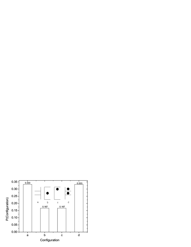
Figure 7: Configurations and residence probabilities for the case $N=3$. Only four states, labeled a, b, c, and d, are possible (inset). The probability of states a and d is 1/3 and the probability of states b and c is 1/6.

A scheme of the possible states for this system is plotted in Fig. 7. Note that the relation between this notation and the more general notation expressed in equations (3), (4) and (5) is $a\equiv(\theta=0)$, $b\equiv(\theta=1,\;j=1)$, $c\equiv(\theta=1,\;j=2)$, $d\equiv(\theta=2)$.

Using the rules of the model, the probabilities of the non-null one-step transitions are: $\mathbf{M}_{a\rightarrow a}=1/3$, $\mathbf{M}_{a\rightarrow b}=1/3$, $\mathbf{M}_{a\rightarrow c}=1/3$, $\mathbf{M}_{b\rightarrow a}=1/3$, $\mathbf{M}_{b\rightarrow b}=1/3$, $\mathbf{M}_{b\rightarrow d}=1/3$, $\mathbf{M}_{c\rightarrow a}=1/3$, $\mathbf{M}_{c\rightarrow c}=1/3$, $\mathbf{M}_{c\rightarrow d}=1/3$, $\mathbf{M}_{d\rightarrow a}=1/3$, $\mathbf{M}_{d\rightarrow d}=2/3$. Thus, for $N=3$, the Markov matrix is

$$\mathbf{M}=\left(\begin{array}[]{cccc}1/3&1/3&1/3&0\\ 1/3&1/3&0&1/3\\ 1/3&0&1/3&1/3\\ 1/3&0&0&2/3\\ \end{array}\right).$$ (32)

The stationary probabilities of residence in this Markov system are the normalized components of the eigenvector of $\mathbf{M}^{T}$ corresponding to the eigenvalue $\lambda=1$, $\mathbf{M}^{T}$ being the transpose of $\mathbf{M}$. These components are

$$\left|\lambda=1\right\rangle=\frac{1}{3}\left(\begin{array}[]{c}1\\ 1/2\\ 1/2\\ 1\\ \end{array}\right),$$ (33)

which agrees with that written in (4) and (6) for any $N$. In the calculation of the probability distribution of the length of the cycles we will follow the general method used in [1], that is

$$P_{N}(n)=\frac{1}{N}[\mathbf{M}^{\prime}]^{n-1}(\theta=0,\,\theta=N-1).$$ (34)

This equations means that the probability of having a cycle of length $n$ is given by $1/N$ times element ($\theta=0,\,\theta=N-1$) of the matrix $[\mathbf{M}^{\prime}]^{n-1}$. This is justified as follows. On the left, we have, by definition, the probability that the cycle lasts $n$ steps. On the right, it is written the probability that, in $n-1$ steps, the system has moved from the empty state to the state with a load $N-1$, with the restriction that this is the first visit to this maximally loaded state. This restriction is easily implemented by making the matrix element $(\theta=N-1,\;\theta=0)$ in $\mathbf{M}$ equal to $0$. That “pruning” converts matrix $\mathbf{M}$ into the new matrix $\mathbf{M}^{\prime}$. Once the system has done this transit in $n-1$ steps, with the mentioned restriction, the probability of passing in one step from the state $\theta=N-1$ to the state $\theta=0$ is $1/N$. This is the reason to include this factor in (34).

In the case $N=2$ the MM [1] and the CM are actually the same model. The $P(n)$ distribution is

$$P_{N=2}(n)=\frac{n-1}{2^{n}}.$$ (35)

In the case $N=3$, $\mathbf{M}^{\prime}$ is

$$\mathbf{M}^{\prime}=\frac{1}{3}\left(\begin{array}[]{cccc}1&1&1&0\\ 1&1&0&1\\ 1&0&1&1\\ 0&0&0&2\\ \end{array}\right).$$ (36)

In order to obtain a generic power of this matrix, we will perform its Jordan decomposition

$$\mathbf{M}^{\prime}=\mathbf{QJQ}^{-1}$$ (37)

and hence

$$\mathbf{M}^{\prime n-1}=\mathbf{QJ}^{n-1}\mathbf{Q}^{-1},$$ (38)

where the factors on the right of (38) are

$$\mathbf{Q} = \left(\begin{array}[]{cccc}0&-2&-\sqrt{2}&\sqrt{2}\\ -1&-1&1&1\\ 1&-1&1&1\\ 0&1&0&0\\ \end{array}\right),$$ (43)

$$\mathbf{J}^{n-1} = \left(\frac{1}{3}\right)^{n-1}\times$$ (48)

$$\left(\begin{array}[]{cccc}1&0&0&0\\ 0&2^{n-1}&0&0\\ 0&0&(1-\sqrt{2})^{n-1}&0\\ 0&0&0&(1+\sqrt{2})^{n-1}\\ \end{array}\right),$$

$$\mathbf{Q}^{-1} = \left(\begin{array}[]{cccc}0&-1/2&1/2&0\\ 0&0&0&1\\ -\frac{1}{2\sqrt{2}}&1/4&1/4&-\frac{4-2\sqrt{2}}{4\sqrt{2}}\\ \frac{1}{2\sqrt{2}}&1/4&1/4&-\frac{-4-2\sqrt{2}}{4\sqrt{2}}\\ \end{array}\right).$$ (53)

Inserting the corresponding formulae into (34), we obtain

$$P_{N=3}(n)=\left(\frac{1}{3}\right)^{n}\left\{-2^{n}+\frac{2-\sqrt{2}}{2(1-\sqrt{2})}(1-\sqrt{2})^{n}+\right.$$ (55)

$$\left.\frac{2+\sqrt{2}}{2(1+\sqrt{2})}(1+\sqrt{2})^{n}\right\},n\geq 2.$$

This function has been plotted in figure 2 together with its numerical counterpart. It is null for $n=2$, as it should, because for $N=3$ the minimum length of a cycle is $3$. It is apparent that $P_{N=3}(n)$ is formed by a combination of three geometric-like terms. This is due to the fact that matrix $\mathbf{J}$ has no off-diagonal term. Inside the brackets the first term is negative, the second is oscillating, and the third –and dominant– is positive. Therefore, in the limit of large $n$ this function is composed only by the third positive geometric decaying term and, in consequence, the asymptotic hazard rate of this model is a constant. The mean $\mu$ and standard deviation $\sigma$ of $P_{N=3}(n)$ are $9$ and $27^{1/2}$ respectively, with an aperiodicity $\alpha=\sigma/\mu=0.58$.

References

References

- [1] M. Vázquez-Prada, A. González, J. B. Gómez, and A. F. Pacheco. Nonlin. Processes Geophys., 9:513, 2002.
- [2] M. Vázquez-Prada, A. González, J. B. Gómez, and A. F. Pacheco. Nonlin. Processes Geophys., 10:565, 2003.
- [3] P. Bak, C. Tang, and K. Wiesenfeld. Phys. Rev. Lett., 59:381, 1987.
- [4] P. Bak, C. Tang, and K. Wiesenfeld. Phys. Rev. A, 38:364, 1988.
- [5] Y. Y. Kagan. Pure Appl. Geophys, 155:537, 1999.
- [6] D. Vere-Jones. Geophys. J. R. Astron. Soc., 42:811, 1975.
- [7] P. Bak and K. Sneppen. Phys. Rev. Lett., 71:4083, 1993.
- [8] K. Ito. Phys. Rev. E, 52:3232, 1995.
- [9] Z. Olami, H. J. S. Feder, and K. Christensen. Phys. Rev. Lett., 68:1244, 1992.
- [10] P. A. Varotsos, N. V. Sarlis, E. S. Skordas, and H. Tanaka. Proc. Japan Acad. Ser. B, 80:429–434, 2004.
- [11] O. Sotolongo and A. Posadas. Phys. Rev. Lett., 92(4):048501, 2004.
- [12] S. Hergarten. Self-Organized Criticality in Earth Systems. Springer, 2002.
- [13] D. Sornette. Critical Phenomena in Natural Sciences. Springer, second edition, 2004.
- [14] V. Kossobokov and Y. Mazhkenov. In D. K. Chowdhury, editor, Computational Seismology and Geodynamics, pages 6–15. American Geophysical Union, 1994.
- [15] D. P. Schwartz and K. J. Coppersmith. J. Geophys. Res., 89:5681, 1984.
- [16] Y. Y. Kagan. Tectonophysics, 270:207, 1997.
- [17] J. C. Savage. Bull. Seism. Soc. Am., 83:1, 1993.
- [18] Alvaro González, Javier B. Gómez, and Amalio F. Pacheco. Am. J. Phys., 73:946, 2005.
- [19] W.I. Newman and D.L. Turcotte. Nonlin. Proc. Geophys., 9:453–461, 1992.
- [20] D. V. Keilis-Bork and A. Soloviev. Nonlinear Dynamics of the Lithosphere and Earthquake Prediction. Springer, 2003.
- [21] G. M. Molchan. Pure Appl. Geophys., 149:233–247, 1997.
- [22] Javier B. Gomez and Amalio F. Pacheco. Bull. Seism. Soc. Am., 94:1960, 2004.
- [23] T. Antal, P. L. Krapivsky, S. Render, M. Mailman, and N. Chakraborty. (and references therein). Phys. Rev. E, 76:041907, 2007.