Multipolar expansion of orbital angular momentum modes

Abstract

In this letter a general method for expanding paraxial beams into multipolar electromagnetic fields is presented. This method is applied to the expansion of paraxial modes with orbital angular momentum (OAM), showing how the paraxial OAM is related to the general angular momentum of an electromagnetic wave. This method can be extended to quasi-paraxial beams, i.e. highly focused laser beams. Some applications to the control of electronic transitions in atoms are discussed.

The angular momentum of light fields continues to draw the interest of the scientific community. Since the work of Allen and coworkers, showing that the angular momentum components of a paraxial light beam, i.e. the spin and the orbital angular momentum (OAM), could be controlled separately Allen et al. (1999), there has been an ongoing discussion regarding concepts as the conservation of angular momentum in different light interaction processes Bloembergen (1969); Berzanskis et al. (1997); Barbosa and Arnaut (2002), the angular momentum flux Barnett (2002) or the measurement of the angular momentum of light Leach et al. (2002); Vasnetsov et al. (2003).

In parallel to this scientific discussion, there has been an explosion of applications of the angular momentum of light, and in particular to the orbital part, covering areas as diverse as trapping and rotating microparticles Grier (2003), astrophysical measurements Harwit (2003); Swartzlander (2006); Thidé et al. (2007) or quantum information Molina-Terriza et al. (2007). Also, recently there has been a renewed interest in the interaction of the orbital angular momentum of light with atomic ensembles Inoue et al. (2006) and the electronic structure of atoms and molecules Alexandrescu et al. (2006).

On the other hand, a general electromagnetic field it is known to have an angular momentum content Jackson (1999). One can even construct solutions to the electromagnetic field with the right spherical symmetries to have well defined values of the total angular momentum and one component of the angular momentum. This kind of solutions receive the general name of multipolar solutions of the electromagnetic field. Up to now, the multipolar fields and the paraxial modes with OAM have been used separately in different regimes. In this letter I try to close this gap and I calculate the multipolar content of any paraxial beam and in particular of the OAM modes.

A general electromagnetic field in free space has two components of the angular momentum (${\mathbf{J}}$): the spin part (hereby denoted by ${\mathbf{S}}$), which is related to the vectorial character of the field, and the orbital angular momentum (OAM) ${\mathbf{L}}$, which is related to the spatial structure of the field Jackson (1999). Both parts are needed to generate rotations in space, and consequently only the combination of the two components plays a meaningful role in the rotational symmetries of an electromagnetic wave, i.e. ${\mathbf{J}}={\mathbf{L}}+{\mathbf{S}}$ Rose (1995). Multipolar modes are precisely a set of solutions to the Maxwell equations which are eigenvectors of the square of the total angular momentum $J^{2}$, one component of the total angular momentum, i.e. the $z$-component, $J_{z}=L_{z}+S_{z}$ and the parity operator. The exact form of these fields can be found for example in Rose (1995). In this letter, I will just use the properties of the vector potential of the multipolar monocromatic fields in the solenoidal gauge. Then following ref. Rose (1995) the vector potentials of the set of multipolar fields is ${\mathbf{A}}_{jm}^{(x)}$, where $x=m$ represents the magnetic multipoles and $x=e$ the electric multipoles. Both classes of multipoles have eigenvalues ${\mathbf{J}}^{2}{\mathbf{A}}_{jm}^{(x)}=j(j+1){\mathbf{A}}_{jm}^{(x)}$ and $J_{z}{\mathbf{A}}_{jm}^{(x)}=m{\mathbf{A}}_{jm}^{(x)}$, but magnetic and electric multipoles differ in their parity. Any given electromagnetic field can be fully expanded onto multipolar fields, if we also add a longitudinal field of the form ${\mathbf{A}}_{jm}^{(l)}={\mathbf{\nabla}}\xi_{j}Y_{jm}$, with $Y_{jm}$ being the usual spherical harmonics.

Let me start by constructing an electromagnetic field by superposing rotated circularly polarized plane waves:

$${\mathbf{A}}=\int_{0}^{\pi}\sin(\theta)d\theta\int_{0}^{2\pi}d\varphi g(\theta,\varphi)R(\theta,\varphi){\mathbf{e}}_{p}\exp(ikz)$$ (1)

where the original plane wave propagates along the $z$ direction and is right (left) handed polarized when $p=1$ ($p=-1$). The altitude and azimuthal rotation angles are given respectively by $(\theta,\varphi)$. The operator $R$, rotates the vector field in the usual manner: $R(\theta,\varphi){\mathbf{e}}_{p}\exp(ikz)=M^{-1}{\mathbf{e}}_{p}\exp(ik\hat{{\mathbf{z}}}\cdot(M{\mathbf{r}}))$. Note that this field is completely general and does not have to fulfil paraxiality. In particular, it can be used to describe beams highly focused with aplanatic lenses Novotny and Hecht (2006). The function $g(\theta,\varphi)$ controls the relative amplitudes of the plane waves.

The main idea of this letter is to find a family of fields using suitable functions $g(\theta,\varphi)$, which in the limit of paraxiality can be identified with the usual orbital angular momentum modes. Let me then develop the rotation operator to the lowest orders in the angle $\theta$ to obtain

$$R(\theta,\varphi){\mathbf{e}}_{p}e^{ikz}\approx e^{ik\theta\rho\cos(\phi-\varphi)+ikz-i\frac{(k\theta)^{2}}{2k}z}(e^{-ip\varphi}{\mathbf{e}}_{p}-\frac{\theta}{\sqrt{2}}\hat{{\mathbf{z}}}),$$ (2)

where I use cylindrical coordinates $(\rho,\phi,z)$. Now, compare this result with a circularly polarized paraxial field of the kind ${\mathbf{A}}={\mathfrak F}_{l}(\rho,z)\exp(ik_{z}z)\exp(il\phi){\mathbf{e}}_{p}$. Any paraxial beam can be expressed as a convenient superposition of this kind of modes Molina-Terriza et al. (2001), so our results apply to any paraxial beam. Besides, this kind of beams are cylindrically symmetric and thus are eigenmodes of both the OAM and the spin AM components in the $z$ direction, i.e. $L_{z}$ and $S_{z}$. Note, however, that this feature is in principle only valid in the paraxial approximation, when $k_{z}\approx k$ and $F_{l}$ is slowly varying in $z$ with respect to $1/k$. This paraxial field can be reexpressed in its Fourier components as ${\mathbf{A}}=\int_{0}^{\infty}k_{r}\,dk_{r}\int_{0}^{2\pi}d\phi_{k}f_{l}(k_{r})\exp(il\phi_{k})\exp(ik_{r}rcos(\phi-\phi_{k}))\exp(ikz-ik_{r}^{2}/(2k)z){\mathbf{e}}_{p}$.

It is clear from inspection of Eqs. (1) and (2) that if we do the correspondence

$$k_{r}=k\sin(\theta),\;\phi_{k}=\varphi,$$

$$g(k_{r}/k,\phi_{k})=k^{2}\,f_{l}(k_{r})\exp\left(i(l+p)\phi_{k}\right),$$ (3)

then the two expansions of the paraxial beam, i.e. in Fourier components and in rotated plane waves Eq. (1), are one and the same, within the paraxial approximation. Then, the set of functions $g$, fulfilling Eq. (3 defines the sought-after family of fields. Note that, in general, we can use functions $f_{l}(k_{r})$ which are not paraxial, thus defining cylindrically symmetric electromagnetic fields.

This identification is useful, because now I will use the expansion of a rotated plane wave into multipole waves Rose (1995, 1955) and perform the integral over the rotation parameters. The expansion reads

$$R(\theta,\varphi){\mathbf{e}}_{p}e^{ikz} = \sum_{j=1}^{\infty}\sum_{m=-j}^{j}i^{j}(2j+1)^{1/2}$$ (4)

$$D_{m\,p}^{j}(\varphi,\theta,0)[{\mathbf{A}}_{jm}^{(m)}+ip{\mathbf{A}}_{jm}^{(e)}],$$

where $D_{m\,p}^{j}(\varphi,\theta,0)$ are the matrices of rotation for irreducible tensors of order $j$. This matrix can be expressed as $D_{m\,p}^{j}(\varphi,\theta,0)=\exp(-im\varphi)d_{m\,p}^{j}(\theta)$, where

$$d_{m\,p}^{j}(\theta) = \left[(j+p)!(j-p)!(j+m)!(j-m)!\right]^{1/2}\times$$ (5)

$$\sum_{s}\frac{(-)^{s}}{(j-m-s)!(j+p-s)!(s+m-p)!s!}\times$$

$$\left(\cos\frac{\theta}{2}\right)^{2j+p-m-2s}\left(-\sin\frac{\theta}{2}\right)^{m-p+2s}.$$

If we put together Eqs. (1),(4) and (5), we obtain

$${\mathbf{A}}=\sum_{j=1}^{\infty}\sum_{m=-j}^{j}i^{j}(2j+1)^{1/2}\int_{0}^{\pi}\sin(\theta)d\theta d_{m\,p}^{j}(\theta)$$

$$\int_{0}^{2\pi}d\varphi\exp(-im\varphi)g(\theta,\varphi)\left[{\mathbf{A}}_{jm}^{(m)}+i{\mathbf{A}}_{jm}^{(e)}\right].$$ (6)

Now, I will use the cylindrically symmetric function $g$ from Eq. (3) to perform the integrals. In this way, the $\varphi$ integral is immediate and the following result holds

$${\mathbf{A}} = 2\pi\sum_{j=\|l+p\|}^{\infty}i^{j}(2j+1)^{1/2}C_{jlp}\left[{\mathbf{A}}_{j\,(l+p)}^{(m)}+i{\mathbf{A}}_{j\,(l+p)}^{(e)}\right]$$

$$C_{jlp} = \int_{0}^{\pi}\sin(\theta)d\theta\,d_{(l+p)\,p}^{j}(\theta)\,f_{l}(ksin(\theta)).$$ (7)

This equation is the main result of this letter. Note that Eq. (7) is a valid solution of the Maxwell equations, as $f_{l}(k_{r})$ is not restricted to paraxial beams, and then can be applied to a wide number of situations. Also, note that all the multipolar beams in the superposition share the same value of $m=l+p$. This has the obvious meaning of summing the OAM and SAM in the paraxial approximation, but in the more general case, simply implies that we have been able to form a family of fields with a well defined $J_{z}$ value. This solution is different from that presented in Refs. Allen et al. (1999); Barnett (2002); Barnett and Allen (1994) and it does not have to fulfil the angular momentum equations derived there.

On the other hand, this result has an interesting side effect. As multipole fields only depend on the wavelength, we can control the multipolar content of a field with only paraxial fields. I will step back a little bit and assume the paraxial approximation again. In this case, the amplitude of the multipolar field of order $(j,m=l+p)$ can be approximated by

$$C_{j\;l\,p}=(-)^{l}\left[(j+p)!(j-p)!(j+l+p)!(j-l-p)!\right]^{1/2}$$

$$\sum_{s}\frac{(-)^{s}}{(j-l-p-s)!(j+p-s)!(s+l)!s!}\frac{M_{l+2s}\{f_{l}\}}{2^{l+2s}}$$ (8)

where the number $M_{a}\{f_{l}\}=\int_{0}^{\infty}k_{r}\,dk_{r}k_{r}^{a}f_{l}(k_{r})$ is the momentum of order $a$ of the function $f_{l}$.

Let me now discuss an important class of functions, the Laguerre-Gaussian modes (LG). The LG modes are defined by two indices, the OAM index, which I conveniently call $l$ and an index stating the number of transversal nodes of the function, which I call $q$. Then, the $f_{l}$ functions read $f_{l,q}(k_{r})=\sqrt{\frac{w_{0}^{2}q!}{2\pi(|l|+q)!}}(w_{0}k_{r}/\sqrt{2})^{|l|}\,L_{q}^{|l|}(w_{0}^{2}k_{r}^{2}/2)\exp(w_{0}^{2}k_{r}^{2}/4+i(q-|l|/2)\pi)$, where $w_{0}$ is the beam width of the LG mode in real space, and $L_{q}^{l}(x)$ are Laguerre polynomials. When this expression is used, the set of momenta $M_{a}$ can be calculated analytically and for the special case of LG modes with $q=0$, we can write the sum in Eq.(8) in a strikingly compact form

$$C_{j;lp}=\sqrt{\frac{(j+p)!(j-p)!(j+l+p)!(j-l-p)!}{(j-\frac{|l|-|l+2p|}{2})!}}$$ (9)

$$k(-)^{j+\frac{l+|l+2p|}{2}}2^{|l|/2+1}w_{0}^{-2j-1+|l+2p|}L_{j-\frac{|l|+|l+2p|}{2}}^{|l+2p|}\left((w_{0}/k)^{2}\right)$$

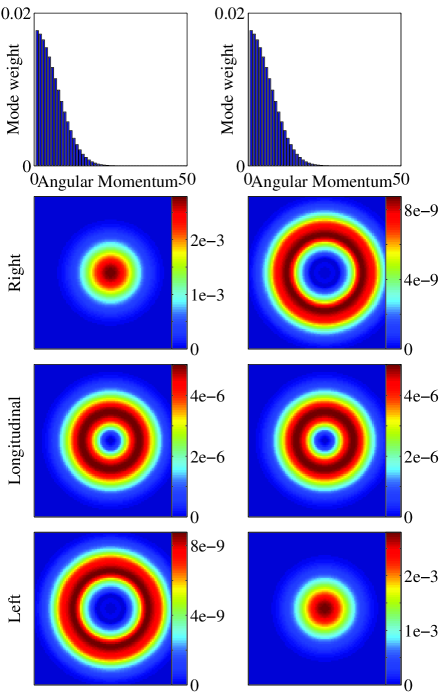
Figure 1: Multipolar decomposition of a Gaussian beam. First column: Right circular polarization ($p=+1$). Second column: Left circular polarization ($p=-1$). First row: weight of the multipolar components $C_{j\;0\,p}^{2}$. Second, third and last rows represent the different components (respectively right circular, longitudinal and left circular) of the field at $z=0$, after performing the summation of the multipole components. Note the different scales for the different components.

I will detail now some examples. The simplest case is that of a paraxial Gaussian beam ($w_{0}\gg 1/k$) with circular polarization. In this case, formula (Multipolar expansion of orbital angular momentum modes) gives the following result

$${\mathbf{A}}=2\pi\sum_{j=1}^{\infty}i^{j}(2j+1)^{1/2}C_{j\;0\,p}\left[{\mathbf{A}}_{j\,p}^{(m)}+ip{\mathbf{A}}_{j\,p}^{(e)}\right]$$

$$C_{j\;0p}=k(-)^{j+1}(j+p)!(j-p)!\sqrt{\frac{1}{(j+\|p\|)!}}$$

$$2w_{0}^{-2j-1+2\|p\|}L_{j-2\|p\|}^{2\|p\|}\left((w_{0}/k)^{2}\right)$$ (10)

Note the following features of this field. First, the field is composed of multipolar solutions with different total angular momentum, but with the same projection of the angular momentum in the direction $z$, which is $+1$ or $-1$ depending on the polarization of the field. Also, in both cases the amplitudes of the multipolar components are the same, as $C_{j;0p}$ does not depend on the sign of $p$. In Fig. (1) we plot the different amplitudes of the multipolar components for $w_{0}=15/k$, and the field resulting when sum (10) is numerically performed.

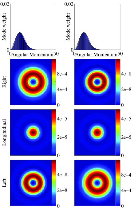
Figure 2: Multipolar decomposition of Laguerre Gaussian beams. First column: Right circular polarization ($p=+1$) and azimuthal index negative ($l=-1$). Second column: Left circular polarization ($p=-1$) and azimuthal index positive ($l=+1$). First row: weight of the multipolar components: $C_{j\;\pm 1\,-l}^{2}$. In this case $C_{j\;+1\,-1}=-C_{j\;-1\,+1}$. Second, third and last rows as in Fig. 1.

Another interesting case occurs when we use Laguerre-Gaussian beam with $l=\pm 1$, $q=0$ and circularly polarized $p=-l$. I have shown that, in the general case, all the multipolar fields have a component of $J_{z}$ is equal to $m=l+p$. Then, in this example the projection of the angular momentum in the $z$ direction of both considered fields is zero, i.e. $m=l+p=0$. The multipolar decomposition gives the following result,

$${\mathbf{A}}=2\pi\sum_{j=1}^{\infty}i^{j}(2j+1)^{1/2}C_{j\;\pm 1\,p=-l}\left[{\mathbf{A}}_{j\,0}^{(m)}+ip{\mathbf{A}}_{j\,0}^{(e)}\right]$$

$$C_{j;l=\pm 1p=-l}=lk(-)^{j}\sqrt{j!(j+p)!(j-p)!}$$

$$2^{1/2+1}w_{0}^{-2j}L_{j-1}^{1}\left((w_{0}/k)^{2}\right)$$ (11)

Note that the weights of the multipoles of the two fields have the same magnitude and opposite signs: $C_{j\;+1\,-1}=-C_{j\;+1\,-1}$. An example of such fields is found in Fig. (2).

This particular example is very interesting as the two considered fields are decomposed in the same subset of multipolar modes: ${\mathbf{A}}_{j\,0}^{(m)}$ and ${\mathbf{A}}_{j\,0}^{(e)}$. This will always be the case of fields with opposite polarizations and $\Delta l=2$. However, in this particular example, both fields share the same weights in the decomposition. This means that if we produce a superposition of the kind: ${\mathbf{A}}=\alpha LG_{10}{\mathbf{e}_{-1}}+\beta LG_{10}{\mathbf{e}_{-1}}$, we can produce a purely transversal electric field when $\alpha=-\beta$ or a pure magnetic one with $\alpha=\beta$. In other cases with opposite polarization and $\Delta l=2$, one can produce a multipole field with a well defined parity just in a set of discrete values of $j$, by playing with the amplitudes of the superpositions and the beam widths of the two fields.

The examples above, and the formulae (7) and (Multipolar expansion of orbital angular momentum modes) demonstrate the control of the superpositions of a set of multipolar fields by using paraxial beams. As considered above, multipolar fields are the solutions of the electromagnetic field one should use when treating spherically symmetric problems. For example, those problems where there is an exchange of angular momentum between the electromagnetic field and material particles are particularly well suited to be treated with multipolar expansions of the electromagnetic field. One such case are the electronic transitions in atoms or molecules. It is well known that multipolar transitions are increasingly more difficult to excite (or de-excite) for larger $j$’s. This is why almost all the literature dedicated to the exchange of angular momentum (or more exactly orbital angular momentum), treats the problem in the dipolar approximation. Actually an easy calculation shows that the probability for a multipolar transition to occur scales as $(a/\lambda)^{2\Delta j}$, with $a$ being the typical radius of the system involved, and $\Delta j$ the multipolar transition Jackson (1999).

Here we are interested in a different, but related problem. Let’s consider the case where it is needed to control a certain multipolar transition. This is the case, for example, when our system is in certain metastable states, as is the case of trapped Ca⁺ ions in quantum information applications Eschner (2005). In those cases the rate of transition is low compared to dipole transitions, simply due to the small size of the ion, compared with the wavelength of the field. Nevertheless, we can still maximize the overlap of the laser beam we are using to induce the transition with the electromagnetic multipole field associated with this transition. Also, in practical applications we have to deal with paraxial or near-paraxial beams. In this situations we can use Eq. (8) to engineer the shape and polarization of our control beam, to maximize the overlap with the desired transition.

Importantly, our method allows to control not only the total angular momentum exchange involved in a certain transition, but also the exchange of $J_{z}$. This can potentially lead to lower losses and errors in some applications, i.e. some quantum information protocols. Our results could be also interesting in the field of nanophotonics where, in some applications one needs to produce light which closely resembles the symmetry of a certain system. It is likely that our method allows to introduce new degrees of freedom in this kind of applications, considering that our equation (7) is valid beyond the paraxial approximation and as stated above, in particular can be used with highly focused beams.

In conclusion, our work closes an existing gap between the descriptions of angular momentum in paraxial and nonparaxial electromagnetic fields. We have demonstrated that a paraxial beam with OAM $l$ and polarization $p$ can be decomposed into multipolar modes with a fixed component of the angular momentum $m=l+p$ and different components of the total angular momentum $j$. We have provided analytical rules to calculate the weight of the superpositions for several interesting cases, thus allowing a control over the superposition of the multipolar fields. These rules could be of utility in fields where the interaction of light and matter has to be controlled with precision.

References

- Allen et al. (1999) L. Allen, M. J. Padgett, and M. babiker, The orbital angular momentum of light (Elsevier, North-Holland, 1999), vol. 39, pp. 291–372.
- Bloembergen (1969) N. Bloembergen, Conservation of angular momentum for optical processes in crystals (Presses Universitaires, Paris, 1969), vol. 109.
- Berzanskis et al. (1997) A. Berzanskis et al, Opt. Commun. 145, 237 (1997).
- Barbosa and Arnaut (2002) G. A. Barbosa and H. H. Arnaut, Phys. Rev. A 65, 053801 (2002).
- Barnett (2002) S. M. Barnett, J. Opt. B: Quantum Semiclass. Opt. 4, S7 (2002).
- Leach et al. (2002) J. Leach et al, Phys. Rev. Lett. 88, 257901 (2002).
- Vasnetsov et al. (2003) M. V. Vasnetsov, J. P. Torres, D. V. Petrov, and L. Torner, Optics Letters 28, 2285 (2003).
- Grier (2003) D. G. Grier, Nature 424, 810 (2003).
- Harwit (2003) M. Harwit, The Astrophysical Journal 59, 1266 (2003).
- Swartzlander (2006) G. Swartzlander, Opt. Photonics News 1, 39 (2006).
- Thidé et al. (2007) B. Thidé et al, Phys. Rev. Lett. 99, 087701 (2007).
- Molina-Terriza et al. (2007) G. Molina-Terriza, J. P. Torres, and L. Torner, Nature Phys. 3, 305 (2007).
- Inoue et al. (2006) R. Inoue et al, Phys. Rev. A 74, 053809 (2006).
- Alexandrescu et al. (2006) A. Alexandrescu, D. Cojoc, and E. D. Fabrizio, Phys. Rev. Lett. 96, 243001 (2006).
- Jackson (1999) J. D. Jackson, Classical electrodynamics (John Wiley and sons, NY, 1999), 3rd ed.
- Rose (1995) M. E. Rose, Elementary theory of angular momentum (Dover publications, Inc., NY, 1995).
- Novotny and Hecht (2006) L. Novotny and B. Hecht, Principles of nano-optics (Cambridge University Press, Cambridge, 2006).
- Molina-Terriza et al. (2001) G. Molina-Terriza, J. P. Torres, and L. Torner, Phys. Rev. Lett. 88, 013601 (2001).
- Rose (1955) M. E. Rose, Multipole fields (John Wiley and Sons, NY, 1955).
- Barnett and Allen (1994) S. M. Barnett and L. Allen, Opt. Commun. 110, 670 (1994).
- Eschner (2005) J. Eschner, in Enrico Fermi Summer School (Varenna, 2005).