Small-tau expansion for the form factor of glued quantum star graphs.

Abstract

We compute the small-tau expansion up to the third order for the form factor of two glued quantum star graphs with Neumann boundary conditions, by taking into account only the most backscattering orbits. We thus show that the glueing has no effect if the number of glueing edges is negligible compared to the number of edges of the graph, whereas it has an effect on the $\tau^{2}$ term when the numbers of glueing and non glueing edges are of the same order.

1 Introduction

The study of the Laplacian on a metric graph, a concept known as quantum graphs, now serves as a toy model for quantum chaos [1, 2, 3]. Indeed, there exists an exact trace formula relating eigenvalues and periodic orbits. Moreover, depending on the graphs, exact computations of these orbits may be possible, whereas they are out of reach in most dynamical systems. It has thus been shown [1, 4, 5] that spectral statistics of simple generic graphs follow random matrix statistics when the size of the graph tends to infinity, as expected for chaotic quantum systems. $V$-star graphs with Neumann boundary conditions (graphs formed by a central vertex connected to $V$ other vertices by edges of different lengths) play a special role because of the high degeneracy of their periodic orbits. As could be expected, this degeneracy breaks the random matrix statistics : this has been shown by the computation of the two-point correlation function ([6, 7]). We will investigate here what happens when two star graphs are glued together. We will first show that glueing two star graphs with $o(V)$ incommensurate bonds has no effect on the form factor when $V$ tends to infinity, and we will next compute the small $\tau$ expansion of two $V$-star graphs glued by $O(V)$ bonds.

Spectral statistics for quantum graphs and the trace formula relating them to periodic orbits will be presented in the first part, as well as a presentation of the model we will be dealing with. The second part will recall the small $\tau$ expansion of the form factor for star graphs as obtained in [7]. In a third part, we will explain our computations in the glued case.

2 Quantum graphs : the trace formula, and the quasar model

We will start by some vocabulary and notations. Let $G=(E,V)$ be a graph with a metric structure : to each edge $(i,j)\in E\subset V\times V$ is assigned a length $l_{ij}$, such that $l_{ij}=l_{ji}$; although the graph is supposed to be non oriented, that is $(i,j)\in E\Rightarrow(j,i)\in E$, and $l_{ij}=l_{ji}$, we will consider the edges to be oriented : $(i,j)$ is different form $(j,i)$, it really describes the edge going from $i$ to $j$). On each edge $(i,j)$, one can thus define a coordinate $x$ such that $x=0$ corresponds to the vertex $i$, and $x=l_{ij}$ corresponds to the vertex $j$. A periodic orbit of period $n$ is a set of $n$ edges $(p_{1},\ldots,p_{n})$ such that $p_{i}$ ends where $p_{i+1}$ starts (as well as $p_{n}$ and $p_{1}$). A periodic orbit is called primitive if it is not the repetition of a shorter periodic orbit. A primitive orbit repeated $r$ times is a non-primitive orbit with repetition number $r$. $\{\mathcal{l}\}$ will denote the equivalence class of all orbits of length $l$. On each edge $(i,j)$, one is looking for the spectrum of the Laplacian. In other words, one wants to find $\lambda$ and $\psi_{ij}$ such that $-\frac{\rmd^{2}\psi_{ij}}{\rmd x^{2}}=\lambda^{2}\psi_{ij}(x)$. As one looks for eigenfunctions defined on the whole graph, one imposes continuity relations at each vertex, $\psi_{ij}(0)=\psi_{ik}(0)$. Moreover, the function should have a unique value on a given point, regardless of the sense of the edge it belongs to : hence one wants $\psi_{ij}(x)=\psi_{ji}(l_{ij}-x)$. This actually corresponds to the Neumann condition on each vertex $\sum_{j}\frac{d\psi_{ij}}{dx}=0$. It is then a simple exercise to check that the eigenvalues $\lambda$ are the solutions of $\det(I-e^{-i\lambda L}S)=0$, where $S$ and $L$ are $|E|\times|E|$ matrices : $L$ is diagonal with the length of each edge as diagonal element, and $S$ is defined by $S_{(i,j),(j,k)}=-\delta_{i,k}+\frac{2}{v_{j}}$, where $v_{j}$ is the number of $j$’s neighbours.

The trace formula as derived in [1] states that if $d(\lambda)=\sum_{n}\delta(\lambda-\lambda_{n})$ is the spectral density, then $d(\lambda)=\frac{L}{2\pi}+\frac{1}{\pi}\sum_{n}\sum_{p\in P_{n}}\frac{l_{p}}{r_{p}}A_{p}\cos(\lambda l_{p})$. Here $L$ is the total length of all edges, $P_{n}$ is the set of all periodic orbits of period $n$ up to cyclic reordering (that is $p_{0},p_{1},p_{2}$ and $p_{1},p_{2},p_{0}$ are the same orbits), $l_{p}$ is the length of the orbit, $r_{p}$ its repetition number, and $A_{p}=\prod_{i=1}^{n}S_{p_{i},p_{i+1}}$.

A $V$-star graph is a graph with vertices $\{0,..V\}$ and edges $E=\{(0,i),(i,0),1\leq i\leq V\}$ : the $V$ vertices are all connected to the center $0$. The $S$-matrix elements for such a graph are $S_{(0,i),(i,0)}=1$ (this corresponds to trivial scattering), $S_{(i,0),(0,i)}=-1+\frac{2}{V}$ (backscattering) and $S_{(i,0),(0,j)}=\frac{2}{V}$ (normal scattering). The lengths will be taken so that they are incommensurate, and that their distribution is peaked around 1 : for instance, they can be chosen randomly, uniformly in $[1-\frac{1}{2V},1+\frac{1}{2V}]$, each length being independent from the others.

We will consider two such $V_{1}$-star graphs and $V_{2}$-star graphs, and connect them with $M$ edges linking the two centers. We will call the resulting graph a $(V_{1},V_{2},M)$ quasar graph, and denote $V=V_{1}+V_{2}+M$. The edges of the two star graphs will be denoted by roman letters ($a,b,$ and so on) and the glueing edges by greek letters ($\epsilon,\zeta,$ and so on).

Figure 1: A quasar graph with $V_{1}=V_{2}=6$ and $M=3$

The $M$ glueing bonds are also supposed to have incommensurate lengths, chosen randomly in $[1-\frac{1}{2V},1+\frac{1}{2V}]$. Hence a periodic orbit of period $2n$ has a length in $[2n-\frac{n}{V},2n+\frac{n}{V}]$; such intervals for different $n$ less than $V$ do not overlap. Of course, in a periodic orbit of period $2n$, each non glueing edge is visited an even number of times (and there is are trivial backscatterings), whereas a glueing edge can be visited an odd number of times (but of course the total number of visits oof glueing edges has to be even). The contribution $A_{p}$ of such an orbit will depend on the number of backscatterings and normal scatterings, and will also depend on the center on which the scattering takes place : it will be a product of factors $r_{i}=(-1+\frac{2}{V_{i}+M})$ (for backscatterings on graph $i$) and $t_{i}=\frac{2}{V_{i}+M}$ (for normal scatterings on graph $i$).

The interesting limit will be the limit $V,n$ tends to infinity with $\tau=\frac{n}{V}$ fixed. In this limit, orbits with the biggest contribution $A_{p}$ will be orbits with the largest number of backscatterings. We will suppose that $V_{1}=\nu_{1}V$ and $V_{2}=\nu_{2}V$, and consider two cases : $M=\nu_{3}V$, or $M=o(V)$.

3 Form factor for the $V$-star graph

The 2-point correlation function is defined as $R_{2}(x)=\left(\frac{2\pi}{L}\right)^{2}\langle d(\lambda)d(\lambda-\frac{2\pi x}{L})\rangle$. The brackets denote a mean value with respect to the $\lambda$’s, that is $\langle f\rangle=\lim_{\Lambda\rightarrow\infty}\frac{1}{2\Lambda}\int_{-\Lambda}^{\Lambda}{f(\lambda)}d\lambda$. Using the trace formula and performing the integral, one gets

$$R_{2}(x)=1+\frac{2}{L^{2}}\sum_{p,p^{\prime}}\frac{l_{p}l_{p^{\prime}}}{r_{p}r_{p^{\prime}}}A_{p}A_{p^{\prime}}\delta_{l_{p}-l_{p^{\prime}}}\cos(\frac{2\pi xl_{p}}{L}),$$

where the sum is over the pairs of periodic orbits $(p,p^{\prime})$, up to cyclic permutations, of lengths $l_{p}$ and $l_{p^{\prime}}$ and repetition numbers $r_{p}$ and $r_{p^{\prime}}$.

The form factor is defined by $K_{st}(\tau)=\int_{-\infty}^{+\infty}(R_{2}(x)-1)\exp(2i\pi x\tau)\rmd\tau$. When $V$ is large, $K^{*}(\tau)$ for $\tau\in[\frac{n}{V}-\frac{1}{2V},\frac{n}{V}+\frac{1}{2V}]$ is well approximated by

$$\frac{V}{L^{2}}\sum_{l}l^{2}(\sum_{p,l_{p}=l}\frac{A_{p}}{r_{p}})^{2}$$

where the first sum is over isometry classes of periodic orbits of period $2n$ and the second is over a given isometry class.

A combinatorial analysis of periodic orbits leads ([7]) to a formula valid near $\tau=0$, yielding a small $\tau$ expansion $K_{st}(\tau)=1-4\tau+8\tau^{2}-\frac{8}{3}\tau^{3}+o(\tau^{4})$.
One should note that the first three terms are given by the orbits consisting of only one edge; to compute the $\tau^{3}$ and $\tau^{4}$ terms, one also needs to take into account the isometry classes of orbits consisting of two or three different edges, but one can then only take into account in these isometry classes the orbits with the maximum number of backscattering (that is, orbits of the form $aa...abb...b$, or $aa...abb...bcc...c$). This approach starts only to fail for the $\tau^{5}$ term, whereas the diagonal approximation fails at $\tau^{4}$ ([6]).

4 The form factor for the quasar graphs if $\nu_{3}=0$

We thus want to compute for $\tau\in[\frac{n}{V}-\frac{1}{2V},\frac{n}{V}+\frac{1}{2V}]$ fixed,

$$K(\tau)=\frac{V}{4V^{2}}\sum_{{\cal{L}}}l^{2}(\sum_{p\in{\cal{L}}}\frac{A_{p}}{r_{p}})^{2}\simeq\tau^{2}V\sum_{{\cal{L}}}(\sum_{p\in{\cal{L}}}\frac{A_{p}}{r_{p}})^{2}$$

Some terms in the sum over equivalence classes concern periodic orbits visiting only one star graph (and no glueing edge). This yields two subsums very similar to the form factor of one star graph : the difference is that in the subsum over the $i$-th stargraph, the number of available vertices is $V_{i}$, whereas the scattering and backscattering factors are $t_{i}=\frac{2}{V_{i}+M}$ and $r_{i}=(-1+\frac{2}{V_{i}+M})$, and not $\frac{2}{V_{i}}$ and $(-1+\frac{2}{V_{i}})$. Nevertheless, if $M=o(V)$, these two sums become in the limit $(n,V)$ tends to infinity $\nu_{1}K_{st}(\frac{\tau}{\nu_{1}})+\nu_{2}K_{st}(\frac{\tau}{\nu_{2}})$, where $K_{st}$ is the form factor for a star graph presented in the preceding section.

We will compute the corrections of the most backscattering orbits to these unglued terms, and check that they disappear in the limit. Since these orbits should give the correct $\tau\rightarrow 0$ asymptotics, this means that the form factor of the quasar graph is in this case $\nu_{1}K_{st}(\frac{\tau}{\nu_{1}})+\nu_{2}K_{st}(\frac{\tau}{\nu_{2}})$, and that the glueing has no effect. In particular, if $\nu_{1}=\nu_{2}=\frac{1}{2}$, one gets $K_{st}(2\tau)$.

Let us consider orbits of length around $2n$ with maximal backscattering, that is orbits consisting only of one glueing edge. Each equivalence class consists of one orbit $\alpha...\alpha$ with repetition number $n$, and $A_{p}=(r_{1}r_{2})^{n}$. There are $M$ such equivalence classes. Hence their contribution to $K$ is $\frac{1}{4V}M(2n)^{2}\frac{(r_{1}r_{2})^{n}}{n^{2}}$ which, when $V,n$ tend to infinity such that $\frac{n}{V}$ is finite, is of the order $\frac{M}{V}$, hence negligible if $M=o(V)$. This is not surprising : there are not enough such terms for them to contribute. This will be the case for all orbits containing glueing edge : to make up for the $\frac{1}{V}$ terms corresponding to normal scatterings, one needs a $V$ combinatorial factor, that one does not get when using glueing edges.

5 The $\nu_{3}\neq 0$ case.

The situation is very different here, since even the two subsums do not give a proper star graph limit. We will thus here compute the exact contributions of the most backscattering orbits of length around $2n$.

5.1 Orbits with no scattering

Let us first examine the case of the no scattering orbits. They consist of one edge, and they can be of three kinds, depending if the edge is a glueing edge or not. In all cases, the equivalence class is a singleton.

If the edge is on star graph $i$, one gets $A_{p}=r_{i}^{n}$ and a repetition number $n$. There are $V_{i}$ such equivalence classes, yielding in the limit $\nu_{i}\exp(-4\frac{\tau}{\nu_{i}+\nu_{3}})=\nu_{i}\exp(-4\tau_{i})$ if one writes $\tau_{i}=\frac{\tau}{\nu_{i}+\nu_{3}}$.

If the edge is a glueing edge, $A_{p}=(r_{1}r_{2})^{n}$ (remember that there is no trivial backscattering for glueing edges). There are $M$ such classes, giving a total contribution of $\nu_{3}\exp(-4\tau(\frac{1}{\nu_{1}+\nu_{3}}+\frac{1}{\nu_{2}+\nu_{3}}))=\nu_{3}\exp(-4(\tau_{1}+\tau_{2}))$.

5.2 Orbits with two scatterings

These are orbits with two different edges. There are three different cases.

If these two edges belong to the same star graph $i$, the weight $A_{p}$ is $t_{i}^{2}r_{i}^{n-2}$. There are $\frac{V_{i}(V_{i}-1)}{2}$ ways to choose the edges, and $n-1$ ways to choose how many times each orbit is visited.

This yields when $V$ tends to infinity a contribution to the form factor $8\tau^{3}\frac{\nu_{i}^{2}}{(\nu_{i}+\nu_{3})^{4}}\exp(-4\tau_{i})=8\tau^{3}\frac{\nu_{i}^{2}}{(\nu_{i}+\nu_{3})^{4}}+o(\tau^{3})$.

If the two edges are glueing edges, there are $M(M-1)/2$ ways to choose them. But the weights depend on the parity of the number of visits of each edge. If it is odd, there is one scattering on star graph 1 and one scattering on star graph 2, hence a weight $A_{p}=t_{1}t_{2}(r_{1}r_{2})^{n-1}$. If it is even, the scatterings can happen either on star graph 1 or on star graph 2 : there are two orbits giving the main contribution in the equivalence class, with respective weights $A_{p}=t_{1}^{2}r_{1}^{n-2}r_{2}^{n}$ and $A_{p}=t_{2}^{2}r_{2}^{n-2}r_{1}^{n}$. Even or odd, there are $n$ or $n-1$ ways to choose how many times each orbit is visited.

All in all, this case yields when $V$ tends to infinity a contribution to the form factor of $8\tau^{3}\nu_{3}^{2}\exp(-4\tau_{2})\exp(-4\tau_{1})(\frac{1}{(\nu_{1}+\nu_{3})^{2}(\nu_{2}+\nu_{3})^{2}}+(\frac{1}{(\nu_{1}+\nu_{3})^{2}}+\frac{1}{(\nu_{2}+\nu_{3})^{2}})^{2})=8\tau^{3}\nu_{3}^{2}(\frac{1}{(\nu_{1}+\nu_{3})^{2}(\nu_{2}+\nu_{3})^{2}}+(\frac{1}{(\nu_{1}+\nu_{3})^{2}}+\frac{1}{(\nu_{2}+\nu_{3})^{2}})^{2})+o(\tau^{3})$

Last, if one of the two edges is a glueing edge and the other one is a $i$-star graph edge, there are $MV_{i}$ ways to choose the edges; there are $n-1$ ways to choose the number of visits of each edge, but the weight depends on it : for example, if $i=1$, and if the glueing edge is visited $n_{e}$ times ($n_{e}$ has to be even), the weight is $A_{p}=t_{1}^{2}r_{1}^{n-2}r_{2}^{\frac{n_{e}}{2}}$. The sum over equivalence classes involves a sum over $n_{e}$ which is a geometric sum; in the limit $V\rightarrow\infty$ one gets a term

$$\tau^{2}\frac{4\nu_{3}\nu_{1}(\nu_{2}+\nu_{3})}{(\nu_{1}+\nu_{3})^{4}}\exp(-4\tau_{1})(1-\exp(-4\tau_{2}))=\tau^{3}\frac{16\nu_{3}\nu_{1}}{(\nu_{1}+\nu_{3})^{4}}+o(\tau^{3}).$$

All in all, the first contribution of the two scatterings orbits to the small $\tau$ expansion of the form factor is a $\tau^{3}$ term equal to

$$8\tau^{3}\left(\frac{1}{(\nu_{1}+\nu_{3})^{2}}+\frac{1}{(\nu_{2}+\nu_{3})^{2}}+\frac{3\nu_{3}^{2}}{(\nu_{1}+\nu_{3})^{2}(\nu_{2}+\nu_{3})^{2}}\right).$$

5.3 $\tau^{3}$ expansion for the $\nu_{3}\neq 0$ case

Putting everything together, the $\tau^{3}$ expansion of form factor for the quasar graph is

$$1-8\tau+8\,{\frac{1+3\nu_{3}}{\left({\it\nu_{2}}+{\it\nu_{3}}\right)\left({\it\nu_{1}}+{\nu_{3}}\right)}}{\tau}^{2}-\frac{8}{3}\,{\frac{{{\it\nu_{1}}}^{2}+14\,{\it\nu_{3}}\,{\it\nu_{1}}+14\,{\it\nu_{3}}\,{\it\nu_{2}}+17\,{{\it\nu_{3}}}^{2}+{{\it\nu_{2}}}^{2}}{\left({\it\nu_{2}}+{\it\nu_{3}}\right)^{2}\left({\it\nu_{1}}+{\it\nu_{3}}\right)^{2}}}{\tau}^{3}+o\left({\tau}^{3}\right).$$

In the particular case $\nu_{1}=\nu_{2}$, (and hence $\nu_{3}=1-2\nu_{1}$), one gets

$$1-8\tau+\frac{16(1-3\nu_{1})}{(1-\nu_{1})^{2}}\tau^{2}-\frac{8}{3}\frac{14\nu_{1}^{2}-40\nu_{1}+17}{(1-\nu_{1})^{4}}\tau^{3}+o(\tau^{3}).$$

The $\tau^{2}$ coefficient is then comprised between $32$ (corresponding to $\nu_{3}=0$) and $36$ (corresponding to $\nu_{1}=\nu_{2}=\nu_{3})$. The difference of the $\tau^{3}$ term with the unglued $\nu_{3}=0$ case is also maximal for $\nu_{1}=\nu_{2}+\nu_{3}$. Yet, even in this case, the two expansions in the glued case and the unglued case are very similar for $\tau\in[0,1]$, so that it is difficult to give numerical evidence. As shown on figure 2, the two form factors are really close to each other until $\tau\simeq 0.15$, and one would then need higher order terms.

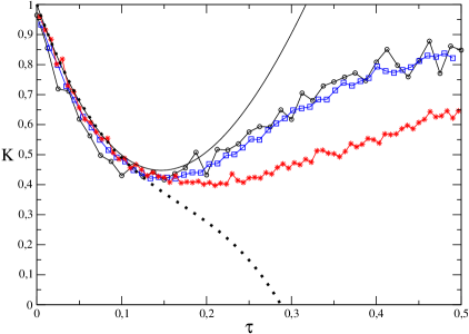
Figure 2: $K^{*}(2\tau)$ (circles), and the form factors for a $(50,50,1)$ quasar graph (squares) and for a $(50,50,50)$ quasar graph (stars). The solid line corresponds to the $\tau^{3}$ expansion in the $\nu_{3}=0$, $\nu_{1}=\nu_{2}$ case, the dashed line corresponds to the $\tau^{3}$ expansion in the $\nu_{1}=\nu_{2}=\nu_{3}$ case.

6 Conclusion

The first effect of the glueing is in the $\tau^{2}$ term : the non-universal statistics of the quantum graph seems to be quite robust. This is not so surprising, since this non universal statistics is strongly linked to the fact that the random walk on the graph converges very slowly to the uniform distribution, and this fact cannot be changed by the glueing. It should be expected that any “star-graph” component of a quantum graph, as long as it is macroscopically big (containing a non-zero fraction of the vertices), should yield a form factor such that $K(0)=1$.

This work benefitted from the support of the french ANR project “Arithmatrix”.

References

References

- [1] T. Kottos and U. Smilansky. Periodic orbit theory and spectral statistics for quantum graphs. Ann. Phys., 274:76–124, 1999.
- [2] S. Gnutzmann and U. Smilansky. Quantum graphs : applications to quantum chaos and universal spectral statistics. Advances in Physics, 55:527–625, 2006.
- [3] F. Barra and P. Gaspard. On the level spacing distribution in quantum graphs. J. Stat. Phys., 101:283–319, 2000.
- [4] T. Kottos and U. Smilansky. Quantum graphs : a simple model for chaotic scattering. J. Phys. A, 36:3501–3524, 2003.
- [5] S. Gnutzmann and A. Altland. Universal spectral statistics in quantum graphs. Phys. Rev. Lett., 93, 2004.
- [6] G. Berkolaiko. Quantum star graphs and related systems. PhD thesis, University of Bristol, 2000.
- [7] G. Berkolaiko and J. P. Keating. Two point spectral correlations for star graphs. J. Phys. A, 32:7827–7841, 1999.