Nonequilibrium spin glass dynamics from picoseconds to 0.1 seconds

Abstract

We study numerically the nonequilibrium dynamics of the Ising Spin Glass, for a time that spans eleven orders of magnitude, thus approaching the experimentally relevant scale (i.e. seconds). We introduce novel analysis techniques that allow to compute the coherence length in a model-independent way. Besides, we present strong evidence for a replicon correlator and for overlap equivalence. The emerging picture is compatible with non-coarsening behavior.

Spin GlassesEXPBOOK (SG) exhibit remarkable features, including slow dynamics and a complex space of states: their understanding is a key problem in condensed-matter physics that enjoys a paradigmatic status because of its many applications to glassy behavior, optimization, biology, financial markets, social dynamics.

Experiments on Spin GlassesEXPBOOK ; LETDYN1 focus on nonequilibrium dynamics. In the simplest experimental protocol, isothermal aging hereafter, the SG is cooled as fast as possible to the working temperature below the critical one, $T<T_{\mathrm{c}}$. It is let to equilibrate for a waiting time, $t_{\mathrm{w}}$. Its properties are probed at a later time, $t+t_{\mathrm{w}}$. The thermoremanent magnetization is found to be a function of $t/t_{\mathrm{w}}$, for $10^{-3}<t/t_{\mathrm{w}}<10$ and $t_{\mathrm{w}}$ in the range 50 s — $10^{4}$ sRODRIGUEZ (see, however,SACLAY ). This lack of any characteristic time scale is named Full-Aging. Also the growing size of the coherent domains, the coherence-length, $\xi$, can be measuredORBACH ; BERT . Two features emerge: (i) the lower $T$ is, the slower the growth of $\xi(t_{\mathrm{w}})$ and (ii) $\xi\sim 100$ lattice spacings, even for $T\sim T_{\mathrm{c}}$ and $t_{\mathrm{w}}\sim 10^{4}$ sORBACH .

The sluggish dynamics arises from a thermodynamic transition at $T_{\mathrm{c}}$EXPERIMENTOTC ; BALLESTEROS ; PALASS-CARACC . There is a sustained theoretical controversy on the properties of the (unreachable in human times) equilibrium low temperature SG phase, which is nevertheless relevant to (basically nonequilibrium) experimentsFRANZ . The main scenarios are the dropletsDROPLET , replica symmetry breaking (RSB)RSB , and the intermediate Trivial-Non-Trivial (TNT) pictureTNT .

Droplets expects two equilibrium states related by global spin reversal. The SG order parameter, the spin overlap $q$, takes only two values $q=\pm q_{\mathrm{EA}}\,.$ In the RSB scenario an infinite number of pure states influence the dynamicsRSB ; FEGI ; CONTUCCI-SEP , so that all $-q_{\mathrm{EA}}\!\leq\!q\!\leq\!q_{\mathrm{EA}}$ are reachable. TNTTNT describes the SG phase similarly to an antiferromagnet with random boundary conditions: even if $q$ behaves as for RSB systems, TNT agrees with droplets in the vanishing surface-to-volume ratio of the largest thermally activated spin domains (i.e. the link-overlap defined below takes a single value).

Droplets isothermal agingSUPERUNIVERSALITY is that of a disguised ferromagnet. A picture of isothermal aging emerges that applies to basically all coarsening systems: superuniversalitySUPERUNIVERSALITY . For $T<T_{\mathrm{c}}\,$ the dynamics consists in the growth of compact domains (inside which the spin overlap coherently takes one of its possible values $q=\pm q_{\mathrm{EA}}$). Time dependencies are entirely encoded in the growth law of these domains, $\xi(t)$. The antiferromagnet analogy suggests a similar TNT Aging behavior.

Since in the RSB scenario $q\!=\!0$ equilibrium states do exist, the nonequilibrium dynamics starts, and remains forever, with a vanishing order parameter. The replicon, a critical mode analogous to magnons in Heisenberg ferromagnets, is present for all $T<T_{\mathrm{c}}$DeDominicis . Furthermore, $q$ is not a privileged observable (overlap equivalenceFEGI ): the link overlap displays equivalent Aging behavior.

These theories need numerics to be quantitativeRIEGER ; KISKER ; MPRTRL_1999 ; BERBOU ; SUE ; SUE2 ; SUE3 ; LET-NUM ; LET-NSU , but simulations are too short: one Monte Carlo Step (MCS) corresponds to $10^{-12}$ sEXPBOOK . The experimental scale is at $10^{14}$ MCS ($\sim 100$ s), while typical nonequilibrium simulations reach $\sim 10^{-5}$s. In fact, high-performance computers have been designed for SG simulationsOGIELSKI ; SUE_DEF ; JANUS .

Here we present the results of a large simulation campaign performed on the application-oriented Janus computer JANUS . Janus allows us to simulate the SG instantaneous quench protocol for $10^{11}$ MCS ($\sim\!0.1$ s), enough to reach experimental times by mild extrapolations. Aging is investigated both as a function of time and temperature. We obtain model-independent determinations of the SG coherence length $\xi$. Conclusive evidence is presented for a critical correlator associated with the replicon mode. We observe non trivial Aging in the link correlation (a nonequilibrium test of overlap equivalenceFEGI ). We conclude that, up to experimental scales, SG dynamics is not coarsening like.

The $D\!=\!3$ Edwards-Anderson Hamiltonian is

$${\cal H}=-\sum_{\langle\bm{x},\bm{y}\rangle}J_{\bm{x},\bm{y}}\sigma_{\bm{x}}\,\sigma_{\bm{y}}\,,\ (\langle\ldots\rangle:\mathrm{nearest\ neighbors})\,.$$ (1)

The spins $\sigma_{\bm{x}}\!=\!\pm 1$ are placed on the nodes, $\bm{x}$, of a cubic lattice of linear size $L$ and periodic boundary conditions. The couplings $J_{\bm{x},\bm{y}}\!=\!\pm 1$ are chosen randomly with $50\%$ probability, and are quenched variables. For each choice of the couplings (one sample), we simulate two independent systems, $\{\sigma_{\bm{x}}^{(1)}\}$ and $\{\sigma_{\bm{x}}^{(2)}\}$. We denote by $\overline{(\cdot\cdot\cdot)}$ the average over the couplings. Model (1) undergoes a SG transition at $T_{\mathrm{c}}=1.101(5)$PELISSETTO .

Our $L\!=\!80$ systems evolve with a Heat-Bath dynamicsVICTORAMIT , which is in the Universality Class of the physical evolution. The fully disordered starting spin configurations are instantaneously placed at the working temperature (96 samples at $T\!=\!0.8\!\approx\!0.73\,T_{\mathrm{c}}$, 64 at $T\!=\!0.7\!\approx\!0.64\,T_{\mathrm{c}}$ and 96 at $T=0.6\approx 0.54\,T_{\mathrm{c}}$). We also perform shorter simulations (32 samples) at $T_{\mathrm{c}}$, as well as $L\!=\!40$ and $L\!=\!24$ runs to check for Finite-Size effects.

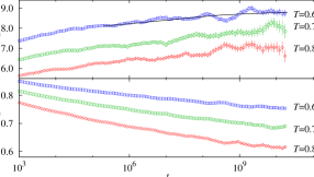
Figure 1: (Color online) Fit parameters, $A$ and $\alpha$ ($C(t,t_{\mathrm{w}})=A(t_{\mathrm{w}})(1+t/t_{\mathrm{w}})^{-1/\alpha(t_{\mathrm{w}})}\,$) vs. $t_{\mathrm{w}}$ for temperatures below $T_{\mathrm{c}}$ ($T\!=\!0.6$ line: fit (for $t_{w}>10^{5}$) to $\alpha(t_{\mathrm{w}})\!=\!\alpha_{0}+\alpha_{1}\log t_{\mathrm{w}}+\alpha_{2}\log^{2}t_{\mathrm{w}}$, $\alpha_{0}\!=\!6.35795$, $\alpha_{1}\!=\!0.18605$, $\alpha_{2}\!=\!-0.00351835$, diagonal $\chi^{2}/\mathrm{dof}=66.26/63$). Coherent oscillations are due to the strong correlations of $\alpha(t_{\mathrm{w}})$ at neighboring times (neither statistical errors nor the fitting curve nor $\chi^{2}/\mathrm{dof}$ vary if one bins data in blocks of 5 consecutive $t_{\mathrm{w}}$).

A crucial quantity in non equilibrium dynamics is the two-times correlation function (defined in terms of the field $c_{\bm{x}}(t,t_{\mathrm{w}})\equiv\sigma_{\bm{x}}(t+t_{\mathrm{w}})\sigma_{\bm{x}}(t_{\mathrm{w}})$)SUE ; KISKER ; RIEGER :

$$C(t,t_{\mathrm{w}})=\overline{L^{-3}\sum_{\bm{x}}c_{\bm{x}}(t,t_{\mathrm{w}})}\,,$$ (2)

linearly related to the real part of the a.c. susceptibility at waiting time $t_{\mathrm{w}}$ and frequency $\omega=\pi/t$.

To check for Full-AgingRODRIGUEZ in a systematic way, we fit $C(t,t_{\mathrm{w}})$ as $A(t_{\mathrm{w}})(1+t/t_{\mathrm{w}})^{-1/\alpha(t_{\mathrm{w}})}\,$ in the range $t_{\mathrm{w}}\!\leq\!t\!\leq\!10t_{\mathrm{w}}$ , obtaining fair fits for all $t_{\mathrm{w}}\!>\!10^{3}\,$. To be consistent with the experimental claim of Full-Aging behavior for $10^{14}\!<\!t_{\mathrm{w}}\!<\!10^{16}$RODRIGUEZ , $\alpha(t_{\mathrm{w}})$ should be constant in this $t_{\mathrm{w}}$ range. Although $\alpha(t_{\mathrm{w}})$ keeps growing for our largest times (with the large errors inSUE it seemed constant for $t_{\mathrm{w}}\!>\!10^{4}$), its growth slows down. The behavior at $t_{\mathrm{w}}=10^{16}$ seems beyond reasonable extrapolation.

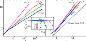
Figure 2: (Color online) Left: SG coherence length $\xi_{1,2}$ vs. waiting time, for $T\!\leq\!T_{\mathrm{c}}$. Right: $\xi_{1,2}$ vs. $I_{1}$, ($\xi_{1,2}\propto I_{1}^{1/(2-a)}$). Also shown data for the 2-D site-diluted Ising model ($L\!=\!4096$, 25% dilution, average over 20 samples, $T\!=\!0.64T^{\mathrm{Ising}}_{\mathrm{c}}$, $\xi_{1,2}$ and $I_{1}$ rescaled by 2 for clarity). Full lines correspond to Ising $a\!=\!0$, (coarsening) and to the SG, $a(T_{\mathrm{c}})\!=\!0.616$PELISSETTO . Inset: $[\xi_{1,2}^{L}(t_{\mathrm{w}})-\xi_{1,2}^{\infty}(t_{\mathrm{w}})]/L$ vs. $\xi_{1,2}^{\infty}(t_{\mathrm{w}})/L$ for $T\!=\!0.8$ and $L\!=\!24,40$ and $80$ ($\xi_{1,2}^{\infty}(t_{\mathrm{w}})$ from a fit $\xi_{1,2}(t_{\mathrm{w}})\!=\!A(T)t_{\mathrm{w}}^{1/z(T)}$ for $L\!=\!80$ in the range $3<\xi_{1,2}<10$, see text).

The coherence length is studied from the correlations of the replica field $q_{\bm{x}}(t_{\mathrm{w}})\equiv\sigma_{\bm{x}}^{(1)}(t_{\mathrm{w}})\sigma_{\bm{x}}^{(2)}(t_{\mathrm{w}})\,$,

$$C_{4}(\bm{r},t_{\mathrm{w}})=\overline{L^{-3}\sum_{\bm{x}}q_{\bm{x}}(t_{\mathrm{w}})q_{\bm{x}+\bm{r}}(t_{\mathrm{w}})}\,.$$ (3)

For $T<T_{\mathrm{c}}$, it is well described byMPRTRL_1999 ; RSB

$$C_{4}(\bm{r},t_{\mathrm{w}})\sim r^{-a}\mathrm{e}^{-\left(r/\xi(t_{\mathrm{w}})\right)^{b}},\quad a\simeq 0.5,\ b\simeq 1.5\,.$$ (4)

The actual value of $a$ is relevant. For coarsening dynamics $a\!=\!0$, while in a RSB scenario $a\!>\!0$ and $C_{4}(r,t_{\mathrm{w}})$ vanishes at long times for fixed $r/\xi(t_{\mathrm{w}})$. At $T_{\mathrm{c}}$, the latest estimate is $a\!=\!1+\eta\!=\!0.616(9)\,$PELISSETTO .

To study $a$ independently of a particular Ansatz as (4) we consider the integrals

$$I_{k}(t_{\mathrm{w}})=\int_{0}^{\infty}\mathrm{d}r\,r^{k}C_{4}(r,t_{\mathrm{w}})\,,$$ (5)

(e.g. the SG susceptibility is $\chi^{\mathrm{SG}}(t_{\mathrm{w}})\!=\!4\pi I_{2}(t_{\mathrm{w}})\,$). As we assume $L\!\gg\!\xi(t_{\mathrm{w}})$ we safely reduce the upper limit to $L/2$. If a scaling form $C_{4}(r,t_{\mathrm{w}})\!\sim\!r^{-a}f(r/\xi(t_{\mathrm{w}}))$ is adequate at large $r$, then $I_{k}(t_{\mathrm{w}})\!\propto\![\xi(t_{\mathrm{w}})]^{k+1-a}\,$. It follows that $\xi_{k,k+1}(t_{\mathrm{w}})\!\equiv\!I_{k+1}(t_{\mathrm{w}})/I_{k}(t_{\mathrm{w}})$ is proportional to $\xi(t_{\mathrm{w}})$ and $I_{1}(t_{\mathrm{w}})\!\propto\!\xi_{k,k+1}^{2-a}\,.$ We find $\xi^{(2)}(t_{\mathrm{w}})\!\approx\!0.8\,\xi_{1,2}(t_{\mathrm{w}})$, where $\xi^{(2)}$ is the noisy second-moment estimateBALLESTEROS . Furthermore, for $\xi_{1,2}\!>\!3$, we find $\xi_{0,1}(t_{\mathrm{w}})\!\approx\!0.46\,\xi_{1,2}(t_{\mathrm{w}})$, and $\xi^{\mathrm{fit}}(t_{\mathrm{w}})\!=\!1.06\,\xi_{1,2}(t_{\mathrm{w}})$, ($\xi^{\mathrm{fit}}$ from a fit to (4) with $a\!=\!0.4$).

Note that, when $\xi\!\ll\!L$, irrelevant distances $r\gg\xi$ largely increase statistical errors for $I_{k}$. Fortunately, the very same problem was encountered in the analysis of correlated time seriesSOKAL , and we may borrow the cure.

The largest $t_{\mathrm{w}}$ where $L\!=\!80$ still represents $L\!=\!\infty$ physics follows from Finite Size ScalingVICTORAMIT : for a given numerical accuracy, one should have $L\!\geq\!k\,\xi_{1,2}(t_{\mathrm{w}})\,.$ To compute $k$, we compare $\xi_{1,2}^{L}$ for $L\!=\!24,40$ and $80$ with $\xi_{1,2}^{\infty}$ estimated with the power law described below (Fig. 2—inset). It is clear that the safe range is $L\geq 7\,\xi_{1,2}(t_{\mathrm{w}})$ at $T\!=\!0.8$ (at $T_{\mathrm{c}}$ the safety bound is $L\geq 6\,\xi_{1,2}(t_{\mathrm{w}})$).

Our results for $\xi_{1,2}$ are shown in Fig. 2. Note for $T\!=\!0.8$ the Finite-Size change of regime at $t_{\mathrm{w}}\!=\!10^{9}$ ($\xi_{1,2}\!\sim\!11$). We find fair fits to $\xi(t_{\mathrm{w}})\!=\!A(T)t_{\mathrm{w}}^{1/z(T)}$: $z(T_{\mathrm{c}})\!=\!6.86(16)$, $z(0.8)\!=\!9.42(15)$, $z(0.7)\!=\!11.8(2)$ and $z(0.6)\!=\!14.1(3)$, in good agreement with previous numerical and experimental findings $z(T)\!=\!z(T_{\mathrm{c}})\,T_{\mathrm{c}}/T$MPRTRL_1999 ; ORBACH . We restricted the fitting range to $3\leq\xi\leq 10$, to avoid both Finite-Size and lattice discretization effects. Extrapolating to experimental times ($t_{\mathrm{w}}\!=\!10^{14}\sim\!100\,$s), we find $\xi\!=\!14.0(3),21.2(6),37.0(14)$ and $119(9)$ for $T\!=\!0.6$, $T\!=\!0.7$, $T\!=\!0.8$ and $T\!=\!1.1\!\approx\!T_{\mathrm{c}}$, respectively, which seem fairly sensible compared with experimental dataBERT ; ORBACH .

In Fig. 2, we also explore the scaling of $I_{1}$ as a function of $\xi_{1,2}$ ($I_{1}\propto\xi^{2-a}$). The nonequilibrium data for $T=1.1$ scales with $a=0.585(12)$. The deviation from the equilibrium estimate $a=0.616(9)$PELISSETTO is at the limit of statistical significance (if present, it would be due to scaling corrections). For $T=0.8,0.7$ and 0.6, we find $a=0.442(11),0.355(15)$ and $0.359(13)$ respectively (the residual $T$ dependence is probably due to critical effects still felt at $T\!=\!0.8$). Note that ground state computations for $L\leq 14$ yielded $a(T\!=\!0)\approx 0.4$GROUND . These numbers differ both from critical and coarsening dynamics ($a\!=\!0$).

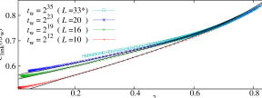
Figure 3: (Color online) For appropriate $t_{\mathrm{w}}$ and $L$, the nonequilibrium $C_{\mathrm{link}}(t,t_{\mathrm{w}})$ vs. $C^{2}(t,t_{\mathrm{w}})$ at $T\!=\!0.7\,,$ coincides with equilibrium $\left.Q_{\mathrm{link}}\right|_{q}$ vs. $q^{2}$ (full lines, data fromULTRA , see text for definitions). The length-time dictionary is $L\!=\!10$ or $t_{\mathrm{w}}\!=\!2^{12}$, $L\!=\!16$ or $t_{\mathrm{w}}\!=\!2^{19}$ and $L\!=\!20$ or $t_{\mathrm{w}}\!=\!2^{23}$. The coherence lengths, $\xi(2^{12})\!=\!2.75(3)$, $\xi(2^{19})\!=\!4.23(4)$ and $\xi(2^{23})\!=\!5.40(7)$, are in the ratio 10:16:20. Hence, from $\xi(2^{35})$, Fig. 2, we predict the equilibrium curve for $L\!=\!33\,$.

We finally address the aging properties of $C_{\mathrm{link}}(t,t_{\mathrm{w}})$

$$C_{\mathrm{link}}(t,t_{\mathrm{w}})=\overline{\sum_{\langle\bm{x},\bm{y}\rangle}c_{\bm{x}}(t,t_{\mathrm{w}})c_{\bm{y}}(t,t_{\mathrm{w}})}/(3L^{3})\,.$$ (6)

Experimentalists have yet to find a way to access $C_{\mathrm{link}}$, which is complementary to $C(t,t_{\mathrm{w}})$ (it does not vanish if the configurations at $t+t_{\mathrm{w}}$ and $t_{\mathrm{w}}$ differ by the spin inversion of a compact region of half the system size).

It is illuminating to eliminate $t$ as independent variable in favor of $C^{2}(t,t_{\mathrm{w}})$, Figs. 3 and 4. Our expectation for a coarsening dynamics is that, for $C^{2}<q_{\mathrm{EA}}^{2}$ and large $t_{\mathrm{w}}$, $C_{\mathrm{link}}$ will be $C$-independent (the relevant system excitations are the spin-reversal of compact droplets not affecting $C_{\mathrm{link}}$). Conversely, in a RSB system new states are continuously found as time goes by, so we expect a non constant $C^{2}$ dependence even if $C<q_{\mathrm{EA}}\,$.

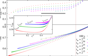
Figure 4: (Color online) Bottom: $C_{\mathrm{link}}(t,t_{\mathrm{w}})$ vs. $C^{2}(t,t_{\mathrm{w}})$ for $T=0.6$ and some of our largest $t_{\mathrm{w}}$ (vertical line: $q_{\mathrm{EA}}^{2}$ fromSUE2 ). We also show our extrapolation of the $C_{\mathrm{link}}$ vs. $C^{2}$ curve to $t_{\mathrm{w}}=10^{14}$ ($\sim 100\,$s, see text). Top: Derivative of $C_{\mathrm{link}}$ with respect to $C^{2}$ for $T\!=\!0.6\,$. The horizontal line corresponds to the slope of a linear fit of $t_{\mathrm{w}}=10^{14}$ extrapolations (the line width equals twice the error). Inset: As in bottom panel, for the ferromagnetic site-diluted $D\!=\!2$ Ising model (same simulation of Fig. 2).

General arguments tell us that the nonequilibrium $C_{\mathrm{link}}$ at finite times coincides with equilibrium correlation functions for systems of finite sizeFRANZ , Fig. 3 ($Q_{\mathrm{link}}$ is just $C_{4}(r=1)$, while $q$ is the spatial average of $q_{\bm{x}}$, Eq.(3)). Therefore, see caption to Fig. 3, we predict the $q^{2}$ dependency of the equilibrium conditional expectation $\left.Q_{\mathrm{link}}\right|_{q}$ for lattices as large as $L=33$.

As for the shape of the curve $C_{\mathrm{link}}=f(C^{2},t_{\mathrm{w}})$, Fig. 4—bottom, the $t_{\mathrm{w}}$ dependency is residual. Within our time window, $C_{\mathrm{link}}$ is not constant for $C<q_{\mathrm{EA}}\,.$ For comparison (inset) we show the, qualitatively different, curves for a coarsening dynamics. Therefore, a major difference between a coarsening and a SG dynamics is in the derivative $\mathrm{d}C_{\mathrm{link}}/\mathrm{d}C^{2}\,,$ for $C^{2}<q_{\mathrm{EA}}^{2}$, Fig. 4—top. We first smooth the curves by fitting $C_{\mathrm{link}}=f(C^{2})$ to the lowest order polynomial that provides a fair fit (seventh order for $t_{\mathrm{w}}\leq 2^{25}$, sixth for larger $t_{\mathrm{w}}$), whose derivative was taken afterwards (Jackknife’s statistical errors).

Furthermore, we have extrapolated both $C_{\mathrm{link}}(t\!=\!rt_{\mathrm{w}},t_{\mathrm{w}})$ and $C(t\!=\!rt_{\mathrm{w}},t_{\mathrm{w}})$ to $t_{\mathrm{w}}\!\approx\!10^{14}$ ($\sim\!100\,$s), for $r\!=\!8,4,\ldots,\frac{1}{16}$. The extrapolated points for $t_{\mathrm{w}}\!=\!10^{14}$ fall on a straight line whose slope is plotted in the upper panel (thick line). The derivative is non vanishing for $C^{2}\!<\!q_{\mathrm{EA}}^{2}\,$, for the experimental time scale.

In summary, JanusJANUS halves the (logarithmic) time-gap between simulations and nonequilibrium Spin Glass experiments. We analyzed the simplest temperature quench, finding numerical evidence for a non-coarsening dynamics, at least up to experimental times (see alsoLET-NSU ). Let us highlight: nonequilibrium overlap equivalence (Figs. 3,4); nonequilibrium scaling functions reproducing equilibrium conditional expectations in finite systems (Fig. 3); and a nonequilibrium replicon exponent compatible with equilibrium computationsGROUND . The growth of the coherence length sensibly extrapolates to $t_{w}\!=\!100$ s (our analysis of dynamic heterogeneitiesLET-NUM ; LET-NSU will appear elsewhereINPREPARATION ). Exploring with Janus nonequilibrium dynamics up to the seconds scale will allow the investigation of many intriguing experiments.

We corresponded with M. Hasenbusch, A. Pelissetto and E. Vicari. Janus was supported by EU FEDER funds (UNZA05-33-003, MEC-DGA, Spain), and developed in collaboration with ETHlab. We were partially supported by MEC (Spain), through contracts No. FIS2006-08533, FIS2007-60977, FPA2004-02602, TEC2007-64188; by CAM (Spain) and the Microsoft Prize 2007.

References

- (1) J. A. Mydosh, Spin Glasses: an Experimental Introduction (Taylor and Francis, London 1993).
- (2) E. Vincent et al., in Complex Behavior of Complex Systems, Lecture Notes in Physics 492.
- (3) G.F. Rodriguez, G.G. Kenning, and R. Orbach, Phys. Rev. Lett. 91, 037203 (2003).
- (4) V. Dupuis et al., Pramana J. of Phys. 64, 1109 (2005).
- (5) Y. G. Joh et al., Phys. Rev. Lett. 82, 438 (1999).
- (6) F. Bert et al., Phys. Rev. Lett. 92, 167203 (2004).
- (7) K. Gunnarsson et al., Phys. Rev. B 43, 8199 (1991).
- (8) M. Palassini and S. Caracciolo, Phys. Rev. Lett. 82, 5128 (1999).
- (9) H. G. Ballesteros et al., Phys. Rev. B 62, 14237 (2000).
- (10) S. Franz, M. Mézard, G. Parisi, and L. Peliti, Phys. Rev. Lett. 81, 1758 (1998); J. Stat. Phys. 97, 459 (1999).
- (11) W. L. McMillan, J. Phys. C 17, 3179 (1984); A. J. Bray, M. A. Moore, in Heidelberg Colloquium on Glassy Dynamics, Lecture Notes in Physics 275; J. L. van Hemmen and I. Morgenstern (ed. Springer, Berlin). D. S. Fisher, D. A. Huse, Phys. Rev. Lett. 56, 1601 (1986) and Phys. Rev. B 38, 386 (1988).
- (12) E. Marinari et al., J. Stat. Phys. 98, 973 (2000).
- (13) F. Krzakala and O. C. Martin, Phys. Rev. Lett. 85, 3013 (2000); M. Palassini and A.P.Young, Phys. Rev. Lett. 85, 3017 (2000).
- (14) G. Parisi and F. Ricci-Tersenghi, J. Phys. A: Math. Gen. 33, 113 (2000).
- (15) P. Contucci and C. Giardina, J. Stat. Phys. 126, 917 (2007); Ann. Henri Poincare 6, 915 (2005).
- (16) D. S. Fisher and D. A. Huse, Phys. Rev. B 38, 373 (1988).
- (17) C. De Dominicis, I. Kondor, and T. Temesvári, in Spin Glasses and Random Fields, edited by P. Young, World Scientific (Singapore 1997).
- (18) J. Kisker, L. Santen, M. Schreckenberg, and H. Rieger, Phys. Rev. B 53, 6418 (1996).
- (19) H. Rieger, J. Phys. A 26, L615 (1993).
- (20) E. Marinari, G. Parisi, F. Ricci-Tersenghi, and J. J. Ruiz-Lorenzo, J. Phys. A 33, 2373 (2000).
- (21) L. Berthier and J.-P. Bouchaud, Phys. Rev. B 66, 054404 (2002).
- (22) S. Jimenez, V. Martin-Mayor, G. Parisi, and A. Tarancón, J. Phys. A: Math. and Gen. 36, 10755 (2003).
- (23) S. Perez Gaviro, J.J. Ruiz-Lorenzo, and A. Tarancón, J. Phys. A: Math. Gen. 39 (2006) 8567-8577.
- (24) S. Jimenez, V. Martin-Mayor, and S. Perez-Gaviro, Phys. Rev. B 72, 054417 (2005).
- (25) L.C. Jaubert, C. Chamon, L.F. Cugliandolo, and M. Picco, J. Stat. Mech. (2007) P05001; H.E. Castillo, C. Chamon, L.F. Cugliandolo, and M.P. Kennett, Phys. Rev. Lett. 88, 237201 (2002); H.E. Castillo et al., Phys. Rev. B 68, 134442 (2003).
- (26) C. Aron, C. Chamon, L.F. Cugliandolo, M. Picco, J. Stat. Mech. P05016, (2008).
- (27) A. Cruz et al., Comp. Phys. Comm. 133, 165 (2001).
- (28) A. Ogielski, Phys. Rev. B 32, 7384 (1985).
- (29) F. Belletti et al., Computing in Science & Engineering 8, 41-49 (2006); Comp. Phys. Comm. 178, 208 (2008); preprint arXiv:0710.3535.
- (30) M. Hasenbusch, A. Pelissetto, and E. Vicari, J. Stat. Mech. L02001 (2008) and private communication.
- (31) See, e.g., D. J. Amit and V. Martin-Mayor, Field Theory, the Renormalization Group and Critical Phenomena, (World-Scientific Singapore, third edition, 2005).
- (32) See e.g. A.D. Sokal, in Functional Integration: Basics and Applications (1996 Cargèse school), ed. C. DeWitt-Morette, P. Cartier, and A. Folacci (Plenum, N.Y., 1997).
- (33) E. Marinari and G. Parisi, Phys. Rev. Lett. 86, 3887 (2001).
- (34) P. Contucci et al., Phys. Rev. Lett. 99, 057206 (2007); P. Contucci, C. Giardina, C. Giberti, and C. Vernia, Phys. Rev. Lett. 96, 217204 (2006).
- (35) The Janus collaboration (manuscript in preparation).