CERN-PH-TH/2008-031
IFT-UAM/CSIC-08-20
Critical gravitational collapse: towards a holographic understanding of the Regge region
Luis Álvarez-Gaumé,111E-mail: Luis.Alvarez-Gaume@cern.ch César Gómez,222E-mail: Cesar.Gomez@uam.es Agustín Sabio Vera,333E-mail: sabio@cern.ch Alireza Tavanfar444E-mail: Alireza.Tavanfar@cern.ch
and Miguel A. Vázquez-Mozo555E-mail: Miguel.Vazquez-Mozo@cern.ch
a Theory Group, Physics Department, CERN, CH-1211 Geneva 23, Switzerland
b Instituto de Física Teórica UAM/CSIC, Universidad Autónoma de Madrid, E-28049 Madrid, Spain
c Institute for Studies in Theoretical Physics and Mathematics (IPM), P.O. Box 19395-5531, Tehran, Iran
d Departamento de Física Fundamental, Universidad de Salamanca, Plaza de la Merced s/n, E-37008 Salamanca, Spain
Abstract
We study the possible holographic connection between the Regge limit in QCD and critical gravitational collapse of a perfect fluid in higher dimensions. We begin by analyzing the problem of critical gravitational collapse of a perfect fluid in any number of dimensions and numerically compute the associated Choptuik exponent in , and for a range of values of the speed of sound of the fluid. Using continuous self-similarity as guiding principle, a holographic correspondence between this process and the phenomenon of parton saturation in high-energy scattering in QCD is proposed. This holographic connection relates strong gravitational physics in the bulk with (nonsupersymmetric) QCD at weak coupling in four dimensions.
1 Introduction
Recently it has been proposed that critical black hole formation might provide the gravitational dual description of diffractive scattering in QCD [1] (see also [2, 3, 4] for other attempts at a holographic description of Pomeron physics). More precisely, the proposal identifies the onset of strong curvature effects in the five-dimensional scalar field gravitational collapse with the corresponding phenomenon in the BFKL evolution, leading to unitarity saturation in QCD in the Regge limit. The computation of the corresponding exponents on the gravity and the QCD side render numerical values that agree quite well.
There are still a number of open questions to be clarified in this conjectured duality. One of them is the reason to consider a scalar field instead of any other kind of collapsing matter. On physical grounds it seems that a perfect fluid would be more appropriate to describe the gravitational dual of hadron scattering. In the center of mass, in the Regge limit, the colliding protons are composed of a large collection of partons, in particular gluons. Hence, a hydrodynamic description, specially when we are interested in collective properties of the scattering process seems appropriate. In this respect it is important to notice that in four-dimensional gravitational collapse one finds that the critical exponents for a collapsing massless scalar field, and for a radiation perfect fluid are numerically very close. The best current value for the Choptuik exponent for a massless scalar field in four dimensions is [5], while for the conformal perfect fluid one has [8, 10]. In five dimensions, the best value for a massless scalar is [5], while in this paper we compute that for a perfect conformal fluid in the corresponding value is . The value to be compared with in the Regge limit of four-dimensional QCD according to [1] is . All these numbers are reasonably “close”, but not close enough that further analysis are not required to establish that they are indeed related by some underlying physics. This implies a double task. On one hand it is necessary to draw a clear enough holographic map between the gravity and the gauge theory descriptions. On the other hand a more precise understanding of the QCD exponents is required.
This paper is divided in two clearly distinct parts. The first part studies a well-posed problem: the determination of the critical exponents in the gravitational collapse of a perfect fluid in dimensions other than four, in particular in five dimensions. The second is dedicated to outline the possible holographic map of this critical collapse with the Regge region. Needless to say, this latter part is wanting a more concrete and straightforward formulation.
The discovery of critical black hole formation has been one of the most exciting developments in numerical general relativity (see [6] for a review). This phenomenon was discovered by Choptuik [7] when studying numerically the spherically symmetric collapse of a massless scalar field. Considering a set of initial conditions parametrized by a real number , such that for “large” a black hole is formed, whereas for “small” the initial scalar field configuration disperses to infinity, it was found numerically that there is a critical value marking the threshold of black hole formation. Surprisingly, for the size of the black hole follows a scaling relation,
| (1.1) |
The critical exponent is independent of the particular family of initial conditions chosen. It changes, however, when the scalar field is replaced by other types of matter.
Notice that the critical solution corresponds to the formation of a “zero mass” black hole. If the scaling behavior (1.1) were observed only in a very restricted value of the parameter close to , the very scaling law would be quite questionable. One could argue that higher curvature corrections to the Einstein equations might wash out this behavior. Indeed, the curvature at the black hole horizon behaves roughly like hence, as the mass goes to zero, the horizon size vanishes and the curvature grows quadratically. Therefore we should expect not only higher curvature effects, but also quantum gravitational effects to become relevant. However, the beauty of Choptuik’s result lies in that the scaling law is observed in a long range of the parameter before the black hole forms. It sets in before the curvature becomes overwhelmingly big. This means that we can expect that there is a region in parameter space where the conjectured holographic map could be defined. Trying to delineate this region is one of the things we attempt in the second part of this paper, although more work remains to be done.
A very interesting feature of the numerical solution found by Choptuik [7] is that when the metric near is approximately discretely self-similar (DSS). This means that the metric functions satisfy the property , with in the case of the spherical collapse of a massless scalar field in four dimensions. This is known as the “echoing” phenomenon. A similar analysis for the case of a perfect fluid collapse [8] shows that the critical solution exhibits continuous self-similarity (CSS) near the center. This implies that there exists a vector field such that
| (1.2) |
where represents the Lie derivative with respect to the vector field .
Space-times with CSS are very interesting from various points of view (see [9] for a comprehensive rewiew). Although DSS is a remarkable phenomenon in gravity, it seems to be a disadvantage when trying to establish a holographic correspondence with the Regge region in QCD, where no echo behavior is to be found. However, the so-called leading -behavior of the amplitudes does indeed show scale invariance (see Section 4). This is a fundamental reason to abandon the construction of the holographic map using collapsing massless scalar fields and to use instead a system where the critical solution exhibits scale invariance. The archetypical system of this kind is the spherical collapse of a perfect fluid.
One of the main (technical) difficulties in the original computation of the Choptuik exponent [7] is that it requires a very involved numerical solution of the Einstein equations. In [8, 10] an alternative procedure to compute was proposed based on a renormalization group analysis of critical gravitational collapse. In this picture, the surface represents a critical surface in the space of solutions separating the basins of attraction of two fixed points, corresponding respectively to Minkowski and the black hole space-times (see Fig. 1). The critical solution with DSS or CSS has a single unstable direction normal to the critical surface.

In this approach, the critical solution is characterized by having a single growing mode for perturbations around it. We can characterize it by the corresponding Lyapunov exponent. If represents the Lyapunov exponent associated to the repulsive direction, the critical exponent is given in terms of it by [10, 6]
| (1.3) |
Consequently, in order to compute the Choptuik exponent associated with a collapsing system, one should identify the critical solutions with either CSS or DSS and look for their single unstable mode.
For systems in which the critical solution has DSS, this renormalization-group approach provides a nice geometrical picture to critical collapse. However, from a practical point of view, the computation of the DSS critical solution still remains a fairly formidable numerical task. If, on the other hand, we deal with systems exhibiting CSS the problem of finding the Choptuik exponent is reduced to numerically solving a system of ordinary differential equations and studying their linear perturbations. For this it suffices to use standard numerical routines to solve the corresponding system of ordinary differential equations, for example Runge-Kutta methods. This is a substantial simplification with respect to simulating the whole system using dynamical triangulations. This is the approach we follow in this paper.
This paper is organized as follows: in Sections 2 and 3 we present the gravitational part of the problem. We start with the study of self-similar, spherically symmetric, solutions to the Einstein equations in dimensions, sourced by a perfect fluid with equation of state . These can be interpreted as critical solutions for the spherical gravitational collapse of a perfect fluid. We write the corresponding equations of motion and study in detail the regularity conditions to be imposed on the solutions. Next, we integrate these equations numerically and study the properties of the solutions. This part has a value on its own. To our knowledge this is the first time such an analysis is carried out. We also present a number of technical clarifications that should be useful to those who would like to engage in similar computations.
Before proceeding to numerically integrate the differential equations there are a number of non-trivial issues that need to be resolved. The Einstein equations with CSS have three singular points in terms of the scaling variable . The solutions near two of them, and , can be dealt with using standard Frobenius analysis. The third, the so-called sonic point, is far more subtle. The generic solution present sonic booms where part of the collapsing matter is thrown out to infinity and part forms a compact object near the origin. For arbitrary initial conditions it is not possible to analytically join the solution below and above the sonic surface. The critical solution is precisely the one that can cross analytically the sonic point (surface). This analyticity constraint implies that there is only a discrete number of possible solutions. The absence of “moduli” in the critical solution adds to the difficulty in its determination. The gravitational part of this paper is essentially the story of how to cross the sonic point, both for the critical solutions as well as their perturbations. This turns out to be a long and winding road we have tried to make as practicable as possible for the reader.
Once the self-similar solution is obtained, we study in Section 3 its perturbations and compute the corresponding repulsive Lyapunov exponent for diverse values of and . From them we obtain the Choptuik exponents in each case, in particular the ones quoted above.
After the detailed discussion of the critical gravitational collapse of a perfect fluid in higher dimensions, in Section 4 we discuss its holographic interpretation in terms of four dimensional high energy scattering in QCD in the perturbative Regge limit.
In Subsection 4.1 we provide a general introduction to the concept of the hard Pomeron as a bound state of two Reggeized gluons. The Reggeization of the gluon at high energies calls for an interpretation in terms of an effective string theory. We are always working in the small ’t Hooft coupling limit in the gauge theory side. However, in deep inelastic scattering (DIS), the gluon distribution function is sensitive to nonperturbative effects not related to confinement: the so-called saturation effects. They are responsible for the transition from a dilute regime, where parton-parton correlations are weak, towards a dense limit where these correlations are very strong. We argue that this dilute-dense transition corresponds to the formation of a higher dimensional tiny black in the gravity side of our holographic proposal.
In Subsection 4.2 a brief introduction to the generalities of evolution equations in DIS is provided. We then focus on the small- limit and describe in some detail the building blocks of the BFKL (Balitsky-Fadin-Kuraev-Lipatov) formalism [14]. The BFKL equation describes a linear evolution of the parton densities with respect to with no ordering in the virtualities of the internal propagators. This generates a UV/IR symmetric random walk in transverse momentum space which can be described by a simple diffusion equation. We identify the variable , proportional to the center of mass energy, as the holographic extra dimension.
The saturated region, corresponding to a dense system of packed partons, is dominated by nonlinearities required to respect the Froissard-Martin bound on total cross sections for very large energies. In Subsection 4.3 the simplest generalization of the BFKL equation containing a nonlinear term, the BK (Balitsky-Kovchegov) equation [15], is introduced. However, we do not use the BK equation in this work since it is posible to study the transition to saturation using an absorptive barrier in the BFKL equation in the limit of asymptotically large center of mass energies. This barrier introduces an asymmetry in transverse momentum space suppressing the propagation towards IR virtualities. These correspond to gluons with a large transverse size and a larger probability of destructive interference. In Subsection 4.4 we discuss the holographic relation between saturation and critical gravitational collapse and argue that the suppression of IR modes in BFKL evolution corresponds to the large fraction of initial matter which evolves into flat space-time in the critical formation of the tiny black hole.
To close the paper, in Section 5 we do not present conclusions, but rather a collection of unanswered questions and work in progress. For the reader’s convenience some technical details have been deferred to the Appendices.
2 Self-similar perfect fluid solutions in dimensions
This is a very long Section where we try to collect in a self-contained way our results on the gravitation collapse of perfect fluids in diverse dimensions. Although we are interested in the case of a conformal fluid in five dimensions, the complexity of the problem is similar in any dimension. Hence we have analyzed the problem including the space-time dimension as a parameter. The basic results are plotted in Figs. 2 to 6, where we exhibit the properties of the critical solutions for a sample of values of in five dimensions. Similar plots could have been shown in other dimensions.
In order to find the Choptuik exponent for the critical collapse of a perfect fluid in dimensions we need to study the corresponding critical solution. In our case this is given by a spherically symmetric self-similar solution of the Einstein equations sourced by a perfect fluid. We begin therefore by obtaining the corresponding Einstein equations.
It is important to stress that one of the difficulties in determining the critical solution in gravitational collapse is that it does not depend on any parameter; or in modern parlance, it generically has no moduli apart from the speed of sound and the dimension of space-time. As a consequence, we have to deal with a system of non-linear differential equations with three singular points that do not seem amenable to analytic treatment in spite of (our) many unsuccessful efforts. In order to obtain numerical solutions that are regular at the singular points we have to toil through a number of steps that we have tried to make as palatable as possible. Once the critical solutions are determined we proceed to study their perturbations and to compute their Lyapunov exponents in the next Section.
2.1 The Einstein equations
Our starting point is then the spherically symmetric -dimensional line element
| (2.1) |
where is the line element on the -dimensional sphere . We look for solutions to the Einstein equations sourced by a perfect fluid with energy-momentum tensor
| (2.2) |
and equation of state
| (2.3) |
We have written the line element (2.1) using comoving coordinates where the components of the fluid velocity are . This is quite standard in the literature. The basic advantage is that the integration of the Bianchi identities is straightforward.
The equations of motion.
The details of the calculation of the Einstein equations for the metric (2.1) can be found in Appendix A. As explained there it is enough to consider the components given by
| (2.4) | |||||
where represents Newton’s constant. The first equations implements the comoving condition with vanishing space-like velocity components for the fluid. These equations have to be supplemented by the Bianchi identities
| (2.5) |
One of the basic simplifying features of studying spherically symmetric gravitational collapse is the fact that gravitational waves are not generated, hence we can write the metric components in terms of the energy-momentum explicitly. General collapse, without spherical symmetry is a far more difficult problem that has not been analyzed yet in the search of critical phenomena. As in the four-dimensional case [11], the equations in (2.4) can be rewritten in a simpler form by introducing the function defined by
| (2.6) |
Together with the Bianchi identities (2.5) we arrive at the following system of equations
| (2.7) | |||||
These equations plus the equations of state (2.3) make a total of six equations to determine the five unknown functions, , , , and . There are therefore only five independent equations. Their physical meaning is transparent. The first one indicates how the mass function defined in Eq. (2.6) grows with the positive energy density . The second implies the decrease of this same mass function induced by a positive pressure. The third gives a measure of the formation of an apparent horizon. Notice that equation (2.6) can be written as the condition when the surface become null. In these coordinates it represents an integral of motion.
The Bianchi identities can actually be written as
| (2.8) |
hence
| (2.9) |
where , are arbitrary functions of and respectively. The function can be absorbed by a redefinition of the radial coordinate . Thus we set in the following.
Special velocities.
There are two families of surfaces in the geometry given by the line element (2.1). The first ones are
| (2.10) |
defining spheres of constant area. The second family of surfaces comes about because we are interested eventually in self-similar solutions. They are defined by
| (2.11) |
One can define now the velocity of these surfaces as the velocity of a fiducial observer lying on one of them with respect to the fluid. This is given by the ratio between the proper distance that this observer covers and the proper time it takes. In the case of the constant- surface we find
| (2.12) |
whereas for surfaces of constant the velocity is
| (2.13) |
Changing coordinates.
Since eventually we are interested in self-similar solutions it is convenient to define the new coordinates by
| (2.14) |
where we have introduced a length scale in order to make the argument of the logarithm dimensionless. Notice that the collapse takes place for , the critical black hole being formed in the limit . This corresponds to the limit . In addition, we introduce the dimensionless functions , and defined respectively by [11]
| (2.15) | |||||
Up to this point we have written the Newton constant explicitly. From now on we use units in which . In this system of units, and have dimensions of (length)2, whereas is measured in units of (length)d-3. The powers of the Newton constant can be restored in all expressions by replacing , and .
Denoting now derivatives with respect to and respectively by a dot and a prime,
| (2.16) |
the Einstein equations become
| (2.17) | |||||
where the dimensionless function is defined by
| (2.18) |
and is given by Eq. (2.13). Both and have been integrated in (2.9) and can now be expressed in terms of the new functions as
| (2.19) |
Thus the velocity is known and we are left with three functions , and [or ] to be determined from the three differential equations in (2.17).
Self-similar solutions.
We now impose self-similarity in the metric (2.1) with respect to the conformal Killing vector field
| (2.20) |
that satisfies Eq. (1.2). In the new coordinates (2.14) the action of the homothety generated by simply shifts the new time variable . Thus, the condition of self-similarity translates into the condition that all dimensionless functions in the problem are independent functions of and depend only of the scaling coordinate . This is the case for the functions defined in Eqs. (2.15) and (2.18). Then, the Einstein equations are (cf. [11])
| (2.21) | |||||
Using the first two equations we can solve for and . The third one can be interpreted as an equation defining as a function of and . Taking its derivative with respect to and after a tedious computation one arrives at the following system of Einstein equations
| (2.22) | |||||
Since in deriving the last equation we have taken a derivative these equations have to supplemented by the third equation in (2.21) at least at a particular point, and also by the expressions for , and
| (2.23) | |||||
where we have fixed the gauge by setting to a constant . Notice that the system still has a residual gauge freedom corresponding to constant rescalings of the time coordinate , with . This implies a rescaling of the constant by . Without loss of generality we require . A very important equation is the form of the velocity field for self-similar solutions. From (2.12) and the self-similar ansatz we can write
| (2.24) |
This equation implies in particular that, if , the zeroes of are in one-to-one correspondence with the values of where .
The sonic point.
The Einstein equations (2.22) present a number of singularities. In principle the possible singularities at and are expected from the fact that we are looking for self-similar solutions. As in the case of regular singularities of linear differential equations, these singularities imply that the solutions have a Frobenius behavior in their neighborhood. Hence they behave as , where the power depends on whether we are at or , but is in any case an analytic function.
The singularity at , the sonic point or sonic surface, is more delicate. It represents the locus where the velocity of the lines of constant reach the speed of sound. At this place shock waves can form. This means that if we start integrating the solution from the origin (or from infinity), we may not be able to cross the sonic surface analytically. Geometrically, the line where is a Cauchy horizon. Choptuik’s critical solution is everywhere analytic, hence we need to impose stringent conditions at the sonic point so that the solution passes through smoothly. These conditions will be explained in detail later.
A generic solution of the system (2.22) depends on three initial conditions. When requiring analyticity throughout, we start by imposing it at the origin. As we will show below this reduces the family of solutions to a one-parameter family. If we also require analyticity at the sonic point, we find that only a discrete set of values of this parameter yield admissible solutions. Generically, the critical solutions have no moduli. They are classified by the zeroes of the velocity field (2.12). In particular, the critical solution we are interested in, the so-called Hunter-A solution [13], is characterized by having a single zero of [12, 11]. The lack of moduli characterizing critical behavior is one of the main difficulties in trying an analytic approach to the solutions of interest. We can easily compute their asymptotic behavior, but close to the sonic point, unfortunately, they only seem to be amenable to numerical analysis.
It is reasonably easy to compute the asymptotic properties of the solution at the origin and at infinity. However if we want to study the solution near the sonic point, we need to impose some restrictions there. In particular regularity of the third equation in (2.22) at imposes the additional constraint
| (2.25) |
This, however, is not enough to determine at the sonic point, since the right-hand side of the corresponding equation is still indeterminate. In order to evaluate this derivative we have to define the right-hand side at the sonic point using l’Hôpital rule
| (2.26) |
As we will show in detail in Subsection 2.2, evaluating the derivatives on the right-hand side of Eq. (2.26) and using the other equations of motion leads to a quadratic equation to be satisfied by at the sonic point. This means that one has to determine which of the two solutions provides the correct analytic solutions connecting smoothly the to through the sonic point. The “wrong” solution would show catastrophic implosion to form a black hole, an explosion to shed all collapsing matter to infinity or something in-between.
In the critical solutions, on the other hand, there is a balance between the matter that collapses and the matter that is ejected, so that eventually we only form a black hole of “zero” mass. It can be shown that once the first derivative of is determined, all higher derivatives can be calculated unambiguously at the sonic point through linear equations obtained by repeated application of the l’Hôpital rule. Indeed, the function can be expanded near in a power series in
| (2.27) |
where . The coefficients are calculable from (2.26) and the equations obtained by taking further derivatives with respect to in the third equation in (2.22). In Subsection 2.2 we evaluate the first coefficient of the expansion, . The details of the calculation of are given in Appendix B.
From the previous discussion it follows that one of the main problems we have to solve is to determine the correct sign in the quadratic equation for . This input is crucial in the numerical evaluation of the critical solution. Before we get there, however, we need to get acquainted with some asymptotic properties of the solutions to Eqs. (2.22).
Behavior near and .
A good place to start the numerical integration of (2.22) in the search of the critical solution is the origin (or infinity). Hence it is worth studying our system of differential equations in these regions. Alternatively, we could start the numerical integration at the sonic point and integrate towards and . Although there are some advantages in doing this, we stick here to and defer the analysis of this other case to a future work [16].
We start the analysis by finding the conditions imposed by analyticity at . By demanding regularity at the origin, we find that the three-parameter family of general solutions to (2.22) reduce to a one-parameter family.
The asymptotic behavior as can be found from the first equation in (2.7). Since for a regular solution is expected to be a single valued function of , Eq. (2.4) can be formally integrated at fixed time
| (2.28) |
For small values of the -coordinate, , one expects the coordinate to vanish. Then the integral can be approximated by
| (2.29) |
Writing now the function defined in Eq. (2.18) in terms of , and , we find its limit when to be
| (2.30) |
It is important to notice that this behavior of the function as is completely general. It does not require the solution to be self-similar, and it is valid as well for the perturbations to the self-similar solution. It only depends on the regularity of the solution at the origin.
Once the limiting value of as has been obtained it is possible to solve the first two equations in the system (2.22) for small . The fact that the value is universal, together with the quadratic relation (2.21), leads to the fact that the asymptotic behavior of the functions , and depends only on a single free parameter. Following [11], we use the constant defined by
| (2.31) |
From Eqs. (2.22) in the limit , together with the gauge condition on the metric coefficient in the same limit, one finds the asymptotic form of , and near as
| (2.32) | |||||
Apart from an overall power of , all functions admit an expansion in integer powers of the variable . It should be noticed that the exponent of the expansion variable never vanishes for physical values of . Incidentally, the constant can be written in terms of as . It is clear from this expression that is a gauge dependent quantity with respect to the residual gauge transformations , . We conclude from this exercise that analyticity at the origin gives a family of solutions depending on a single parameter .
A further restriction on the possible values of comes from requiring that the solution is analytic at the other singular value of , the sonic point . Generically we find that only a discrete set of values of lead to a regular solution for all finite values of . These correspond to the higher-dimensional generalization of flat-Friedmann, general relativistic Larson-Penston and Hunter-A/B solutions [11]. How these solutions are found numerically is discussed in detail in Sec. (2.3).
The behavior of the functions in the limit can also be obtained using similar techniques. It can be shown that all functions , and tend to constants in that limit and that from the equations of motion (2.22) it follows that when . Looking at the subleading terms, the expansion is of the form
| (2.33) |
for any of the relevant functions collectively represented here by . All functions near can be expanded in inverse power series in the variable . This expansion parameter is different from the one appearing when expanding the functions around . It is important to notice that this expansion parameter is independent of the dimension. Furthermore, if we look at the expression for in (2.23), we find that its absolute value diverges at precisely as . In fact, provides a good uniformizing variable for the system of equations under study. Indeed, is a monotonic function in the whole region between and . This variable is essentially the one used in the analysis of Ref. [17]. We turn now to study the form of the field equations in terms of this variable. This will be helpful in determining the correct sign of at the sonic point.
The uniformization variable.
One unpleasant aspect of the equations obtained so far is the presence of generically irrational exponents in both the equations and the initial conditions. This problem can be solved by choosing an appropriate uniformization variable in terms of which integer powers are obtained. This can be done by noticing that the expansion of around has the form
| (2.34) |
We have seen before how all functions, apart from an overall power of , can be written as series expansion in . Therefore, by redefining the functions properly in such a way that all the Frobenius factors are absorbed, it should be possible to write them as a series expansion in integer powers of . Moreover, for critical solutions is a monotonous function of that can be used as the independent variable.
We begin by defining a new function as
| (2.35) |
Using this new function together with and , the system (2.22) can be rewritten as
| (2.36) | |||||
After the introduction of all functions appear with integer exponents on the right-hand side of the equations. At the same time the parameter appears explicitly in the system to be solved.
The velocity vanishes in the limit . Similarly, the function has a simple behavior in that limit as a function of , namely
| (2.37) |
This shows that is a good candidate to be used as independent variable. With this choice, the functions and satisfy the following system of differential equations
This system can be integrated in principle by requiring regularity at the sonic point . Notice that in these variables the regularity at these points leads again to the condition (2.25). As a bonus, using these variables we eliminate the constant from the initial conditions at to make it appear explicitly in the equations. In integrating the system numerically we can use either Eqs. (2.22) or Eqs. (LABEL:eqs_background). Both systems are equivalent, although the conceptual advantage of the parametrization is that near the regular singular points the functions can be expanded in integer powers of this variable.
Once the functions and are known, it is possible to find their dependence on the scaling coordinate by integrating the last equation in (2.36) to find . This procedure gives the same values of for the regular solutions as the ones obtained integrating the equations in terms of the independent variable . The fact that the values of are the same is a consequence of the fact that in writing the equations (LABEL:eqs_background) we have not changed the gauge fixing conditions.
Shooting from the sonic point666This paragraph can be read independently of the main argument line. The reader can skip this paragraph without losing the thread of the arguments. In a future publication [16] we plan to present the numerical integration from the sonic point towards the origin and infinity. . The system of ordinary differential equations (2.22) can also be integrated from the sonic point . In this case it is convenient to fix the residual gauge freedom, , by locating the position of the sonic point at a given value of the scaling coordinate, . In this case the constant is fixed by the equation defining the sonic point,
| (2.39) |
where the subscript “sp” indicate that the corresponding function is evaluated at the sonic point.
In the same way as the behavior of the solutions near the origin is determined by a single parameter , the requirement of regularity at the sonic point forces now that the values of the functions at this point depend on just one free parameter. We can take this to be the value of the function at the sonic point, . To see this we notice that there are two conditions that the functions should satisfy at the sonic point, namely the regularity condition (2.25) and the quadratic equation in (2.21)
| (2.40) |
The quantity can be now written in terms of by using the definition of the function in Eq. (2.18), whereas . In this way it is possible to solve the previous two equations for and as a function of . Moreover, by requiring analyticity of the functions at it is possible to show that all derivatives of the functions at that point are also determined by .
Thus, we have found then that there is a one-parameter family of solution to the system (2.22) regular at the sonic point. Only when we require in addition that the corresponding functions also show the behavior described previously as the set of allowed functions restrict to a finite set of values of the initial condition . These allowed values for each correspond to different types of solutions associated with the values of giving regular solutions everywhere.
It is interesting to relate the initial condition at the sonic point with the parameter governing the asymptotic behavior of the regular solution at . The key ingredient to do this is to notice that the condition together with Eq. (2.39) gives the following relation between and
| (2.41) |
where as shown above and are given in terms of . The explicit dependence of this expression on the “gauge fixing parameter” shows once more that is a gauge-dependent quantity. In addition, from this expression it is immediate to verify that the combination is gauge invariant.
2.2 Dealing with the sign ambiguity.
Let us go back to the determination of at the sonic point. The last step that we need to solve before embarking in the numerical solution of the self-similar Einstein equations is to fix somehow the ambiguity associated with the choice of the right solution to the quadratic equation satisfied by . This leads to a long and involved calculation. This is, in fact, one of the prices one has to pay for using comoving coordinates. In Schwarzschild coordinates a similar problem appears [10] but it is technically easier to solve. If the reader is willing to give us the credit that we have solved the problem, this subsection can be skipped. The result however is very important in the numerical determination of the critical solution.
To see how the quadratic equation for comes about we go back to Eq. (2.26). In order to evaluate the right-hand side of this equation we need the expressions for , and evaluated at the sonic point. For the first one we use the expression of in Eq. (2.23) to write
| (2.42) | |||||
where in the second line we have used the field equations (2.21) to write the logarithmic derivatives in terms of the values of the functions at the sonic point. For we find also from Eq. (2.23)
| (2.43) |
Finally, the derivative of the function can be written as
| (2.44) |
Substituting these expressions in Eq. (2.26) leads to the following quadratic equation for
| (2.45) | |||
As discussed above, the values of all functions at the sonic point can be expressed in terms of a single parameter that we can choose to be . This means that the coefficients of the quadratic equation (2.45) can be written in terms of this single parameter. To do this we solve Eqs. (2.40) for the combinations and with the result
| (2.46) |
Substituting now these expressions in Eq. (2.45) we arrive at
| (2.47) | |||
As advertised, all coefficients depend only on .
This quadratic equation can be written in the canonical form as
| (2.48) |
where the coefficients are given by
| (2.49) |
The first thing to be noticed is that the equation for is independent of and therefore it is gauge invariant, as it is to be expected. Solving the equation
| (2.50) |
There is therefore an ambiguity in the value of given by the two possible signs in this equation.
The numerical integration of the equations (2.26) from the origin shows that, for both the Hunter-A/B solutions, is determined by the minus branch in Eq. (2.50). For these types of solutions, this branch is automatically selected by the system when regularity at both the origin and the sonic point is imposed, i.e. when the constant takes the corresponding critical values. The situation changes if we start the integration from the sonic point. In this case we find that the “correct” branch in Eq. (2.50) has to be chosen in order to determine the right initial conditions for the numerical integration. This situation will be addressed in detail in a separate publication [16].
2.3 Numerical analysis
After this long study of the properties of the equations of motion (2.22) for the self-similar background, we can proceed to integrate the equations numerically. To do so we use a fourth-order Runge-Kutta routine that integrates the system starting at . As explained before, the main difficulty lies in finding the right value of providing an analytic solution at the sonic point. For a generic value of the routine gives a solution that diverges at this point.
In order to find the right value we perform a scan in to find the smooth numerical solution at the sonic point . Since we look for solutions that can be interpreted as describing critical gravitational collapse of a perfect fluid, we are interested in the solution with a single unstable mode. In dimension larger than four, this corresponds to the higher-dimensional generalization of the general relativistic Hunter-A solution, which are characterized by single zero of the function .
The numerical analysis is a bit delicate due to the singular character of the sonic point, where minor numerical noise can easily lead one astray. Here it is important to use the analytical information we have at hand: the behavior of the solution at the origin and the value of the derivatives of the relevant functions at the sonic point. After long numerical work, we have determined the critical solutions for different values of in various dimensions, in particular and . We have included the computation in our analysis in order to compare with previous work, in particular Ref. [10].
In Figs. 2 and 3 we have plotted the profile of the main functions for three values of in five dimensions. The position of the sonic point is denoted by a dot on the corresponding curve. We see that the curves have a structure completely similar to their four-dimensional counterparts, as found for instance in Ref. [11].
Fig. 4 shows how the function is monotonic in the whole range of values of . This demonstrates that this function can be used as a good independent variable to describe the evolution of the system.
Finally, in Figs. 5 and 6 we plot the various functions of interest against instead of . This is useful to show that we have indeed found the critical solution. As explained before the critical solutions are characterized by the zeroes of the velocity field (see Fig. 3). What Figs. 5 and 6 show is a form of critical damping. The solution tends to its asymptotic value at after turning around it only once. Critical solutions with more than one zero in would spiral around their value at infinity a number of times given by the number of zeroes of this velocity field. Notice that cannot be used to uniformize the problem, because it is not monotonous as a function of . However, the fact that only crosses the value (at which ) at a single finite value of before monotonously decreasing to as is also a sign that the solution is critical. Indeed, the relation between and given in Eq. (2.24) shows that for the critical solution can be also characterized as the one for which the function crosses the value at a single finite value of .


3 Perturbations of the self-similar solutions
Once we have obtained the critical self-similar solutions we proceed to study their stability by considering perturbations around them. The perturbations break self-similarity and therefore have an explicit dependence. In the context of critical gravitational collapse we are interested in solutions with a single growing mode. The analysis is long, and in particular we need to use a very relevant equation that does not seem to appear in the literature (see the paragraph on the -equation). The sonic point, together with a new singularity that appears in the perturbation equations at , play an important rôle in the analysis. Similarly to the calculation of the self-similar brackground, analyticity at all singular points gives the key to the computation of critical exponents.
3.1 Analysis of the perturbations.
The equations for the perturbations.
Let us denote by any of the functions involved in the problem. We consider perturbations around the self-similar solution of the form
| (3.1) |
where is the corresponding Lyapunov exponent. Since we are interested in the mode that grows as , the unstable mode is associated with a positive value of . The dots in the equation include the contribution of stable modes with negative Lyapunov exponents.
In order to write a set of differential equations for the perturbations , and we have to go back to the full equations of motion (2.22) and plug in the ansatz (3.1). Then we collect all the terms linear in the expansion parameter . From the first two equations in (2.17) we find the equations of the perturbations and to be
| (3.2) |
We still lack one more equation for the perturbation of a third function that we chose to be . To find it we have to use the third equation in (2.17) and expand to first order in . After a long calculation one arrives at
| (3.3) |
where all the “coefficients” are functions of given by
| (3.4) | |||||
Expressions (3.2) and (3.3) give the relevant equations governing the perturbations. We can actually reduce them to a system of two differential equations by plugging the value of the perturbation , obtained from Eq. (3.3), into Eqs. (3.2). As a result one gets the following system of two first order differential equations for the perturbations and
| (3.5) |
where , , and are given respectively by
| (3.6) | |||||
Singularities and the -equation.
As in the case of the background equations one has to be careful about potential singularities in the equations for the perturbations. In particular, by looking at the expression of in Eq. (3.3) and the form of the coefficients , and , we find that there are singular points corresponding to the zeroes of . This can happen at three points. The first one is again the sonic point where . The second point is the value of at which . The third possibility, , is never realized for physical solutions with because the function is always positive definite.
In the case of the self-similar background, regularity at the sonic point implied the extra condition (2.25) to be satisfied by the physically admissible solutions. In the case of the perturbations an extra condition can be also extracted by considering the perturbations of the quadratic equation in (2.21) in a consistent way. In particular we take the derivative of this equation with respect to and express the result in terms of the functions , and . After these manipulations the resulting expression can be written as a linear equation for of the form
| (3.7) |
where the coefficients and are given in terms of the functions , and their derivatives.
For the self-similar ansatz, Eq. (3.7) reduces to the second equation in (2.22). If, on the other hand, we consider perturbations of the self-similar solution this expression contains important information about the regularity of the perturbed solution at the points at which vanishes. To see this, we insert the perturbations (3.1) into (3.7) and use Eqs. (3.2) and (3.3) to obtain a relation between and . A long computation yields
| (3.8) |
where and are respectively given by
and
The coefficients , , , and are the ones defined above. We see that the only poles in and come from the zeros of , i.e. the points at which , and . Thus, Eq. (3.8) can be written as a sum of terms potentially divergent at plus those which are regular at those points. After some manipulations we find that this equation has a structure of the form
| (3.11) |
where we have introduced the coefficient defined by
In order to preserve the identity (3.11) one must require that the whole expression is regular at the zeroes of . Since numerically it can be shown that never vanishes at those points we arrive at the conclusion that
| (3.13) |
In particular, this equation has to be satisfied at the sonic point and provides a nontrivial condition to be satisfied by the perturbations there.
Notice that this condition has been derived here as a straightforward consequence of the perturbations of Eq. (3.7), which becomes trivial after imposing the self-similar ansatz. It should be said that Eq. (3.13) plays a basic rôle in the determination of the Lyapunov exponents of the critical solutions, and that to our knowledge it has never appeared in previous literature. Without including it, the path to understanding the properties of critical perturbations is rather treacherous. A systematic computation of the Choptuik exponents for different values of and relies heavily on it.
Behavior of the perturbations at the sonic point.
In order to negociate the singularities of the differential equation (3.3) we impose analyticity at the singular points. For this we have to use again the l’Hôpital rule to define the perturbation in terms of the corresponding ones for the other functions. This means that in the regions near the points where we can replace Eq. (3.3) by
| (3.14) |
At the same time, instead of using Eq. (3.5) we consider the modified system
| (3.15) |
The new coefficients , , and are given by
| (3.16) | |||||
| (3.17) |
where the function is defined by
| (3.18) |
In order to solve the previous system, the derivatives of the different coefficients are required. To keep here the exposition simple, these expressions are given in Appendix C.
Decoupling of the perturbations.
In this paragraph we show how the perturbations and can be decoupled from one another. Although outside the mail line of the paper, the analysis presented here may provide a different way to understand the perturbations to the critical solutions. In any case the paragraph can be skipped in a first reading.
Going back to the equations for the perturbation (3.5), we can formally integrate each of the equations to find the following system of integral equations for and (keep in mind that the prime indicates derivation with respect to )
| (3.19) |
Using again (3.5) they become
| (3.20) |
Taking now a derivative with respect to on both equations, and after some manipulations, we arrive at a set of two decoupled second-order linear differential equations for the perturbations and
| (3.21) |
where the coefficients are given by
| (3.22) | |||||
The system of equations (3.21) can be written in a more suggestive form by a further function redefinition
| (3.23) |
where the new functions and satisfy one-dimensional Schrödinger equations
| (3.24) |
The potentials for these equations are given in terms of the coefficients of Eq. (3.21) by
| (3.25) |
Hence, we can obtain the perturbations to the self-similar background by solving a system of two Schrödinger equations with the appropriate boundary conditions. The potential associated with these equations is completely determined by the self-similar solution. Once (3.24) is solved, the perturbations for the other functions, and , can be written in terms of and . This formulation of the pertubations can provide a good arena for qualitative analysis. We will however proceed with a direct study of the original equations.
Asymptotic behavior of the perturbations near and .
In order to solve the perturbations , and by integration of the system of differential equations (3.5) starting at we need to determine the behavior of these functions at the origin. To do so, we start by noticing that the function (including the perturbation) should have the limiting value determined in Eq. (2.30). Because this condition is satisfied already by the self-similar background solution we conclude that the perturbation has to vanish in this limit
| (3.26) |
Hence, studying the system (3.2) around one arrives at the identity
| (3.27) |
For positive (as it is the case of the growing mode we are interested in), the integration of this equation results in the combination blowing up at as . Therefore, in order to impose regularity of the perturbations at the origin we require the numerical coefficient of this divergent terms to be zero. This leads to the condition
| (3.28) |
Equations (3.26) and (3.28) give the initial conditions for the numerical integration of the system of differential equations (3.2) at . Notice that since we have a linear system, only the ration at the origin is relevant. Furthermore, the same conclusions can be reached from the equations determining from and together with standard asymptotic analysis at .
The functions and can be written, around , as a power series. From the reduced system of equations (3.15) it can be seen that they can be expressed as
| (3.29) |
Comparing with Eq. (2.32) we learn that the expansion variable here is the same as the one for the self-similar background solution.
We now consider the behavior of the perturbations at infinity. Since in that limit the function tends to one, we find that the system of equations (3.2) simplifies for large to
| (3.30) |
leading to
| (3.31) |
For the growing mode, , this means that the combination vanishes at infinity as
| (3.32) |
To get the individual behavior of and we look at the asymptotic form of for large . From Eq. (3.3), using the asymptotic expansion of the background functions when , we arrive at
| (3.33) |
Plugging this in Eq. (3.2) we get the following equations, valid for large ,
| (3.34) |
implying
| (3.35) |
To summarize, we have found that for (the growing mode) all perturbations , and go to zero at infinity as powers of . On the other hand, for small the only perturbation that vanishes is , while and tend to constants in that limit satisfying the condition (3.28).
The gauge mode.
In studying the perturbations to the self-similar solutions of the Einstein equations it is very important to eliminate those perturbations which can be written as mere gauge transformations of the background solutions. In particular, by performing changes of coordinates on the self-similar solutions it is possible to introduce an explicit dependence on time that is just a gauge artifact. One can consider reparametrizations in time [10], leaving invariant the form of the line element (2.1). Infinitesimally
| (3.36) |
This changes the scaling coordinate by
| (3.37) |
where the function is defined in terms of as
| (3.38) |
The functions , and only change under (3.36) through their dependence on . In the case of the self-similar solutions we find
| (3.39) |
where stands for , and . This has precisely the form of the perturbation (3.1) if we choose the arbitrary function of the form
| (3.40) |
with any real constant. The perturbations , and are then given by
| (3.41) | |||||
Using the behavior of the self-similar solutions near it is straightforward to see that the perturbations (3.41) automatically satisfy the boundary condition (3.28). However, in order to satisfy the boundary condition at we find from (2.33) that the Lyapunov exponent has to be
| (3.42) |
In particular, we see that the gauge mode is independent of the space-time dimension.
3.2 Numerical study of the perturbations and calculation of the Choptuik exponent
As in the case of the self-similar solution, the equations for the perturbations have to be numerically integrated using the background solutions obtained numerically in Sec. 2.3. We use a strategy similar to the one applied there. We numerically integrate the system (3.5) starting at using a fourth-order Runge-Kutta routine. We find that for generic values of the Lyapunov exponent the perturbation is singular both at the sonic point and at the value where . We then scan in to find a critical value for which the solution smoothly crosses both points. At the same time we ignore the value of associated with the gauge mode. The singularities of the equations lead to some numerical instabilities, but the use of l’Hôpital rule explained above gives a guidance to the numerical integration. A good deal of work leads to the results for the Choptuik exponents in Table 1 for dimensions and . As an important check of our results we agree with previous results in [10, 11].
| 0.01 | 8.747 | 4.435 | 3.453 | 3.026 |
|---|---|---|---|---|
| 0.02 | 8.140 | 4.288 | 3.376 | 2.974 |
| 0.03 | 7.617 | 4.152 | 3.302 | 2.924 |
| 0.04 | 7.163 | 4.027 | 3.233 | 2.876 |
| 0.05 | 6.764 | 3.911 | 3.169 | 2.831 |
| 0.06 | 6.412 | 3.804 | 3.107 | 2.788 |
| 0.07 | 6.099 | 3.703 | 3.049 | 2.746 |
| 0.08 | 5.818 | 3.609 | 2.993 | 2.706 |
| 0.09 | 5.565 | 3.521 | 2.940 | 2.668 |
| 0.10 | 5.334 | 3.438 | 2.890 | 2.631 |
| 0.11 | 5.124 | 3.360 | 2.841 | 2.595 |
| 0.12 | 4.932 | 3.286 | 2.795 | 2.561 |
| 0.13 | 4.756 | 3.216 | 2.751 | 2.527 |
| 0.14 | 4.593 | 3.149 | 2.708 | 2.494 |
| 0.15 | 4.442 | 3.086 | 2.667 | 2.464 |
| 0.16 | 4.301 | 3.026 | 2.627 | 2.433 |
| 0.17 | 4.170 | 2.968 | 2.589 | 2.414 |
| 0.18 | 4.048 | 2.913 | 2.552 | 2.377 |
| 0.19 | 3.933 | 2.860 | 2.517 | 2.348 |
| 0.20 | 3.825 | 2.809 | 2.482 | 2.321 |
| 0.21 | 3.723 | 2.760 | 2.449 | 2.297 |
| 0.22 | 3.627 | 2.713 | 2.417 | 2.272 |
| 0.23 | 3.536 | 2.668 | 2.386 | 2.246 |
| 0.24 | 3.449 | 2.625 | 2.355 | 2.224 |
| 0.25 | 3.367 | 2.583 | 2.325 | 2.202 |
| 0.01 | 0.114 | 0.225 | 0.290 | 0.330 |
|---|---|---|---|---|
| 0.02 | 0.123 | 0.233 | 0.296 | 0.336 |
| 0.03 | 0.131 | 0.241 | 0.303 | 0.342 |
| 0.04 | 0.140 | 0.248 | 0.309 | 0.348 |
| 0.05 | 0.148 | 0.256 | 0.316 | 0.353 |
| 0.06 | 0.156 | 0.263 | 0.322 | 0.359 |
| 0.07 | 0.164 | 0.270 | 0.328 | 0.364 |
| 0.08 | 0.172 | 0.277 | 0.334 | 0.369 |
| 0.09 | 0.180 | 0.284 | 0.340 | 0.375 |
| 0.10 | 0.187 | 0.291 | 0.346 | 0.380 |
| 0.11 | 0.195 | 0.298 | 0.352 | 0.385 |
| 0.12 | 0.203 | 0.304 | 0.358 | 0.390 |
| 0.13 | 0.210 | 0.311 | 0.364 | 0.396 |
| 0.14 | 0.218 | 0.318 | 0.369 | 0.401 |
| 0.15 | 0.225 | 0.324 | 0.375 | 0.406 |
| 0.16 | 0.232 | 0.330 | 0.381 | 0.411 |
| 0.17 | 0.240 | 0.337 | 0.386 | 0.416 |
| 0.18 | 0.247 | 0.343 | 0.392 | 0.421 |
| 0.19 | 0.254 | 0.347 | 0.397 | 0.426 |
| 0.20 | 0.261 | 0.356 | 0.403 | 0.431 |
| 0.21 | 0.259 | 0.362 | 0.408 | 0.435 |
| 0.22 | 0.276 | 0.368 | 0.414 | 0.440 |
| 0.23 | 0.283 | 0.375 | 0.419 | 0.445 |
| 0.24 | 0.290 | 0.381 | 0.425 | 0.450 |
| 0.25 | 0.297 | 0.387 | 0.430 | 0.454 |
In Figs. 7 and 8 we show the plots of , and versus for three different values of . As expected, all perturbations go to zero at large , whereas only vanishes in the limit . This means that, for constant , self-similarity is mostly broken near whereas the symmetry is restored at large values of . In particular, we see that the position of the sonic point (marked by a dot in the plots in Figs. 7 and 8) approximately indicates the value of where , and begin to decay towards zero.
Notice, however, that the perturbations to the self-similar solution come multiplied by where is the positive Lyapunov exponent. This means that the region where CSS is broken grows as increases until at some point the linear perturbation regime becomes invalid. The system goes then into a full nonlinear regime that, for supercritical solutions, results in the formation of a black hole in the asymptotic future.
In Figs. 9 and 10 we plot the perturbations in terms of . As in the case of the critical solution, this shows that the perturbations reach their asymptotic values at after a single turn. Once again this shows that we have correctly identified the most relevant perturbations leading to the computation of the critical exponents.
The regularity of the perturbations at the sonic point fully determine the value of the Lyapunov exponent . In Table 1 we show the values of both and the Choptuik exponent for various values of in four, five, six and seven space-time dimensions. All values shown in this table are given with a precision of . These values of the Lyapunov and Choptuik exponents are the main concrete result of this paper. Looking at the value obtained for the conformal fluid in five dimensions , , we find it is reasonably close to the value for a massless scalar field. This situation is very similar to the four-dimensional case, where the Choptuik exponent for a conformal fluid is very close to the value of a massless scalar field. This is also the case for the conformal fluids in () and (), as compared to the values of the Choptuik exponents for the collapse of a massless scalar field in these dimensions [5]. Furthermore the value of the Choptuik exponent for the conformal perfect fluid in is also close to the BFKL exponent as calculated in [1]. To what extent this numerical agreement is serendipity or a sign of something deep will be analyzed in the next Section.


4 A holographic glimpse through the Regge region
4.1 Nonperturbative physics at weak ’t Hooft coupling
Probably the most important lesson we have learned from Maldacena’s conjecture [19] is that the QCD string, i.e. the effective string defining the representation of Yang-Mills Wilson loops as sums over random surfaces, is the fundamental string in some higher dimensional geometry [20]. In spite of many efforts during the last ten years, we are still lacking the concrete string background geometry for QCD. However, many of the results so far obtained hint at the existence of a close relation between nonperturbative effects in QCD and black hole dynamics in the gravity dual picture.
An interesting perturbative regime where stringy aspects of QCD naturally appear is the Regge limit of scattering amplitudes. In this region the center of mass energy is much larger than all the other Mandelstam invariants in the process under consideration, . There also exists some hard scale, , which allows for a perturbative treatment of the problem. Although the coupling is small, the amplitudes are dominated by logarithms of , making a resummation of terms of the form mandatory. Note that is the usual ’t Hooft coupling. This resummation can be performed using the BFKL [14] formalism which predicts a Regge behavior of the type for total cross sections, with being some effective Regge trajectory. When the quantum numbers exchanged in the -channel are those of the vacuum, the dominant trajectory is that of the BFKL Pomeron (also known as hard Pomeron since it is of perturbative origin).
In the leading logarithmic approximation (LLA), where coupling and large logarithms carry the same power in the resummed terms, at asymptotically large energies and in the physical region of negative the BFKL Pomeron trajectory goes like . This power-like behavior of the cross sections calls for modification since it violates unitarity bounds at very high energies. In the context of deep inelastic scattering (DIS) and evolution equations for parton distribution functions, the onset of unitarity can be interpreted in terms of “saturation” corrections which tame the power-like growth with . The physics of saturation is driven by perturbative degrees of freedom, because we are far away from the confinement region. However, the treatment of the problem is nonperturbative since it corresponds to the description of a very dense system. The main target of this Section is to provide a holographic or gravity dual description of these non perturbative saturation effects.
The gravity dual interpretation of the BFKL Pomeron has been previously addressed in [2]. Using a string target space in the ultraviolet of type AdS5 it is possible to study the hard Pomeron at strong ’t Hooft coupling . This is done by computing perturbative string amplitudes in the Regge limit with being the small perturbation parameter, where is the string scale, the curvature radius and . In this weak gravity limit the BFKL diffusion in transverse momentum is mapped into propagation along the curved holographic direction. The physics of diffusion in time at weak and strong ’t Hooft coupling is qualitatively the same but with different coefficients.
Let us remark that in this holographic correspondence the BFKL Green’s function in the weak gravity side, computed in a small curvature gravitational background, is mapped to the large BFKL Green’s function in the gauge theory side computed around the saddle point “background” of the BFKL kernel eigenvalue . As we will explain in the next Subsections, the nonperturbative phenomena of saturation requires to move to a different saddle point background where amplitudes are not power-like anymore at large and enjoy “geometrical scaling”. In the gravity dual picture this change of saddle point “BFKL” background should correspond to a nonperturbative change of gravitational background. This new background would require to take into account off shell gravity effects and therefore is beyond the semiclassical weak gravity limit.
In Ref. [21] multi–Regge kinematics was extended to include nonperturbative effects in the region of small momentum transfers of the BFKL equation in a string theory. In Ref. [22], assuming that the hard Pomeron intercept in SYM equals the graviton one in AdSS5, it was possible to obtain a very good extrapolation of DIS anomalous dimensions of twist–2 operators from weak to strong coupling.
After this brief introduction we now move to a more detailed description of our holographic picture. We start with an introduction to the calculation of scattering amplitudes in the Regge limit of perturbative QCD.
4.2 Deep inelastic scattering and BFKL
Let us start with a short introduction to DIS at small values of Bjorken . In very simple terms, in DIS we are resolving the structure of a large target, e.g. a hadron, with an electromagnetic probe. This probe is typically a photon with virtuality and transverse size . In the target’s rest frame we can think of the photon’s wave function as forming perturbatively well before the interaction with the target. When the transverse size of the photon is small it goes through the target like a “needle”, however, for smaller virtualities the leading component of the photon’s wave function, a quark-antiquark pair, is dressed with a color cloud of higher order gluonic components. In this case the -hadron cross section behaves very similarly to that of hadron-hadron scattering (see Ref. [23] for a review).
In a leading twist picture, the virtual photon resolves partons in the hadron carrying a fraction of its longitudinal momentum. This takes place with a probability , the so-called parton distribution function. The evolution with of is well described in perturbation theory using the DGLAP formalism [24]. As the hadron is a complicated strong interacting object it is not possible to calculate the parton distribution functions from first principles. Nevertheless, very good fits to experimental data have been achieved by assuming a certain nonperturbative functional form for the dependence of the parton distribution at a close to the confinement scale and evolving it to larger scales using perturbative evolution equations. Collinear factorization theorems ensure that, if the final is large enough, these parton distribution functions are universal: they can be measured in DIS experiments in electron-hadron machines and then used for predictions at hadron-hadron colliders. The region of is well understood from the experimental and theoretical sides.
The situation in the limit is far more complicated. In principle, even if is large enough as to ensure a small value for the strong coupling, it turns out that the cross sections or structure functions are dominated by logarithms of which are very large as we enter this region. This implies that terms of the form should be resummed to all orders to get an accurate description of the data. The resummation of these terms can be effectively carried out by means of the BFKL [14] evolution equation, which can be considered as orthogonal to DGLAP in the kinematic plane. While DGLAP is based on perturbative splittings where one emission is ordered in transverse momentum with respect to the previous one, BFKL stems from strong ordering in longitudinal components. After integration over the phase space of these emissions a power like growth of the form is obtained for . When the resummation is of leading logarithms in , i.e. if the power in the coupling is the same as that of the logarithm then, for
| (4.1) |
When one power of the logarithm is lost we are in the next-to-leading order approximation and is smaller.
The BFKL equation in LLA has been rederived in many different ways in the literature. The original calculation was based upon the study of scattering amplitudes in the so-called multi-Regge kinematics. There are two main ingredients: the elastic scattering amplitude for the process and the inelastic amplitude for . We focus on gluons since their splitting function dominates at small .
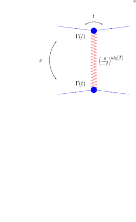
When we consider the scattering amplitude in the Regge limit of it has a simple factorized form in terms of two external -dependent functions and an energy dependence of the form . In DIS, and the limit of large corresponds to small physics. This exponentiation of the logarithms in energy is known as Reggeization of the gluon (see Fig. 11). If we project on the gluon’s quantum numbers in the -channel this means that, while at lowest order in we have the usual gluon propagator, when higher orders are taken into account this propagator is modified by the Regge factor above–mentioned. The gluon then lies on a Regge trajectory, , which, as usual, reproduces the gluon’s spin when is equal to the gluon mass, i.e. . In more detail, we have
| (4.2) |
where and is an infrared regulator.
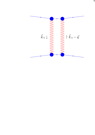
It is possible to construct a perturbative Pomeron with the quantum numbers of the vacuum if we exchange two Reggeized gluons and project the amplitude on a color singlet. In this case the four-point amplitude can be written as
| (4.3) |
where are the two-dimensional transverse momenta of the incoming gluons. Note that the transverse components of the four momenta decouple from the longitudinal ones. These are integrated out in multi-Regge kinematics with the Bjorken variable playing the rôle of a cutoff. Thus we can consider as the cutoff of the effective theory for the transversal degrees of freedom and the BFKL equation as the renormalization group evolution in “” time.
Let us indicate that Eq. (4.3) corresponds to the amputated gluon Green’s function since for zero Y we get the normalization
| (4.4) |
which corresponds to the -channel exchange of two normal gluons.
It is interesting to remark some simple facts derived from Eq. (4.3). The trajectory in Eq. (4.2) is a negative function, which means that the elastic scattering amplitude in Eq. (4.3) decreases as the energy grows. The delta function in Eq. (4.3) imposes conservation of transverse momenta but it also means that we can consider the evolution of a Reggeized gluon as the action of a diagonal operator acting on some basis in the transverse momentum space.
Being a color singlet, the BFKL Pomeron does not radiate and it is responsible for “diffractive” events, where there are regions in the detector without hadronic activity, the so-called “rapidity gaps”. To make connection with total cross sections or structure functions we can use the optical theorem. In this way we can relate the imaginary part of the forward elastic amplitude with the total cross section. This means that we can use Eq. (4.3) with to obtain a first contribution to .
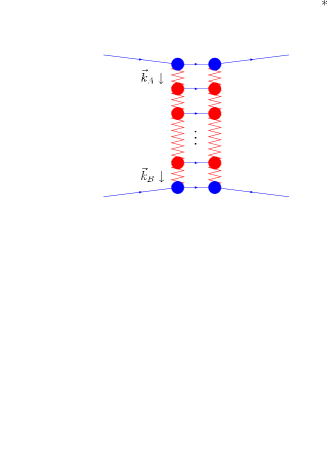
As it stands, Eq. (4.3) is not an infrared safe quantity since it has an explicit dependence on . This dependence is eliminated when we include the second ingredient in the BFKL equation: the inelastic amplitude. This amplitude is calculated in multi-Regge kinematics where the three outgoing gluons are well separated in rapidity from each other. This gives rise to a gauge invariant effective emission vertex. When this vertex is included we have that the gluon Green’s function in the forward case now reads
| (4.5) | |||||
where
| (4.6) |
and (see Fig. 13). Below we will show a simpler representation where the dependence on the infrared regulator explicitly disappears. Before this we would like to point out that the action of the real emission kernel is not diagonal in transverse space anymore, as can be clearly seen in the second line of Eq. (4.5). This will be an important point when connecting with gravitational theories. It is also worth noting that the Green’s function without virtual terms would be
| (4.7) | |||||
this means that the real emission makes grow very rapidly as we move towards smaller values of . Let us note that both competing effects in Eq. (4.3) and Eq. (4.7) depend on the infrared regulator .

Making use of bootstrap, the virtual and real contributions to the BFKL amplitude can be combined in such a way that the infrared parameter is eliminated. This brings the following simpler representation for the Green’s function
| (4.8) |
where
| (4.9) |
is the eigenvalue of the BFKL kernel and is the logarithmic derivative of Euler’s Gamma function. is the azimuthal angle formed by the two–dimensional vectors and . Its Fourier conjugate variable can be interpreted as a conformal spin in elastic scattering. The dominant region of integration is . Around this point we can see in Fig. 14 that the eigenvalue of the kernel is positive only for . This implies that the dependence on is only important at low energies and we can keep for our arguments. Hence, we average over the azimuthal angle
| (4.10) | |||||
where and, from now on, .
Let us now study the structure of this equation for very large values of . We can write
| (4.11) |
and evaluate the integral using the saddle point approximation around the minimum of at
| (4.12) |
to obtain the expression
| (4.13) |
with . This asymptotic expansion is driven by the first exponential, which contains the leading behavior in energy, with being the Pomeron intercept given in Eq. (4.1). The function has poles at integer values of with the physical region corresponding to . The poles at are related to virtualities in the internal propagators smaller and larger, respectively, than the external scales. The terms containing are sensitive to the shape of at its minimum and indicate the speed of propagation into the infrared and ultraviolet regions. It is easy to verify that the function
| (4.14) |
asymptotically fulfills the diffusion equation
| (4.15) |
This diffusion in transverse momentum is IR/UV symmetric as a consequence of the invariance of under the transformation .
The gauge/string duality has offered the possibility to explore the sector of DIS with the hope of building the correct string dual of QCD. In the dipole approximation to DIS a holographic description at strong ’t Hooft coupling was obtained in terms of a semiclassical approximation to the light-like Wilson loop in the target metric. At finite temperature and in the quark–gluon phase this was done using the AdS black hole metric in [25]. Another interesting study was carried out in Ref. [26] where structure functions were calculated at strong ’t Hooft coupling. The model is based on supersymmetric Yang-Mills (SYM) theory broken down to at a given mass scale. When going to the small limit the analysis was performed within the single string picture. This set up is limited since, as we will see in the coming Subsections, new effects in the gauge theory side related to the onset of unitarity indicate that one should better operate with multi-string configurations. A more complete analysis of this region was presented in Ref. [3]. In that work, rather than resumming multi–loop string amplitudes, inspiration is taken from perturbative QCD to understand the flow towards unitarity at large and the gravity effect on a “bulk” photon of large virtuality is worked out semiclassically. This photon is defined using any of the gauge fields in the bulk associated with the global -symmetries of the theory. With increasing virtualities of this probe the transition to unitarity changes from a single–Pomeron picture to one with multiple graviton exchanges.
In the present work we investigate unitarization effects in DIS in the limit of weak ’t Hooft coupling and very large center of mass energy. In this limit the LLA, where terms of the form are resummed, is accurate since higher order corrections are always suppressed by larger powers in the coupling, e.g. the next–to–leading order approximation (NLLA) resums terms. The NLLA corrections in SYM have been studied in [27]. The program to construct even higher order corrections in this theory was initiated in [28].
It is important to note that we are not working with a supersymmetric theory from the beginning. It is the dynamics of our process, treated in multi–Regge kinematics, what provides a highly symmetric effective theory at high energies. As a matter of fact, in the LLA, the BFKL kernel is the same in QCD or super Yang–Mills theories. This is because fermions are suppressed at high energies and their effects are only important at higher orders in the approximation. Moreover, we are not sensitive to the running of the coupling since the Feynman diagrams contributing to it do not belong to the LLA because they bring an extra power in without generating a logarithm in energy. Last, but not least, this theory naturally shows planarity which comes as a consequence of the LLA.
We follow a bottom–up approach and find that the perturbative description of the saturation line, to be defined in detail below, within the BFKL formalism shares many interesting features with the critical formation of a tiny black hole in higher dimensions. Our approach to the identification of the Regge holography will be mostly constructive. The first issue is to identify the holographic extra dimension. Since in the BFKL approach to the Regge limit we are working with an effective theory parametrized by , we define the holographic coordinate as , the natural energy scale in the problem. In the mapping of BFKL dynamics to critical black hole formation we consider the evolution in the holographic variable as dual to time evolution in the gravitational collapse. At the threshold of formation of the black hole the variations in the metric components are large and should be well described within a perturbative analysis in the gauge theory side.
The next step in our description should be to identify the geometry on the holographic direction. This geometrical information for Regge holography should be hidden in the BFKL kernel , with parameterizing a particular gravitational background. In the AdS/CFT correspondence, in order to describe a phase transition, we need to deal with the full quantum gravity canonical ensemble of metrics with a given boundary topology. In our case, to describe the transit through the saturation region, which corresponds to the flow from a dilute partonic regime to a dense system, we need to consider the full ensemble of BFKL backgrounds weighted by the kernel . In the next Subsection we will try to put some substance to these general guiding lines of work.
4.3 Unitarity in DIS and perturbative saturation
It is well known that the LLA in Eq. (4.13), predicting a power-like growth in energy for total cross sections, violates the unitarity bound set by Froissart. The problem of unitarization of cross sections at high energies is a very complicated one. From a perturbative point of view it can be understood by introducing a new set of Feynman diagrams. In the context of QCD Reggeon field theory a new vertex arises: that of the transition from Reggeized gluons. This “triple Pomeron vertex” is invariant under transformations [29], a Möbius invariance also present in the BFKL Hamiltonian in the non-forward case [30]. In the large limit the triple Pomeron vertex in QCD reduces to the vertex used in the Balitsky-Kovchegov (BK) equation [15]. This equation describes a DIS process where the target is an extended and dense object. The effect of taking into account unitarity in this equation is to introduce a non-linear piece added to the usual BFKL kernel. Neglecting impact parameter effects and azimuthal angle dependence, the BK equation can be written as
| (4.16) | |||||
with the initial condition fixed by
| (4.17) |
The non–linear term in Eq. (4.16) arises from the introduction of fan diagrams and it has a mild effect at the beginning of the evolution, when the gluon amplitude is small. The growth is therefore power-like at early times in . On the contrary, for large values of , when the amplitude is larger, unitarity appears in the form of nonlinearities and the quadratic term in Eq. (4.16) becomes very important since it completely suppresses the growth of the amplitude with energy. In terms of parton densities this transition to a saturated state can be understood as the crossover from a dilute system of partons within the hadron to a very dense one which can be interpreted as a “color glass condensate” (CGC) [31].
As we already remarked, the precise dynamics of unitarization requires to take into account multi-Pomeron vertex effects. However, it is still possible to describe within a single Pomeron picture some general features such as scaling laws present in the crossover to the saturation region. For this we closely follow [32].
We are considering the limit of very large energies and we can start by evaluating the integral in Eq. (4.11) asymptotically. It is important to correctly identify the virtuality corresponding to the target in the DIS process, in Eq. (4.11), and that of the projectile, . We can then write
| (4.18) |
At it is possible, for fixed values of and Y, to find the –background that dominates asymptotically. It is implicitly given by the saddle point condition
| (4.19) |
To evaluate the Green’s function we now expand around this saddle point
| (4.20) |
and obtain
| (4.21) |
where . The leading behavior of this expression is driven by the first exponential. The remaining pieces are of diffusive origin and do not need to be considered in a first analysis. The growth with energy of Eq. (4.21) is dictated by the function which we plot in Fig. 15.

This function is monotonically decreasing as grows. It has a zero at the point
| (4.22) |
For any in the physical interval (0,1) the kernel is positive. For we have that is negative and Eq. (4.21) rises very rapidly as Y gets larger. In the range , changes sign but its value is not large enough as to stop the growth of the Green’s function. However, for backgrounds with there is no growth because is so large that it forces the amplitude to decrease with energy. The value at which this change in behavior takes place is
The value is precisely where the derivative of the kernel cancels, , and where the usual BFKL expansion happens. It generates a rise of the cross sections which must be tamed at some point in energy in order to respect unitarity bounds. Unitarity can be enforced in our single Pomeron picture if we impose the extra constraint that the dominant region of integration at asymptotic Y corresponds to . What we obtain is
| (4.23) |
with , and In the kinematic plane of DIS, the critical line where the transition to saturation occurs can be read off the saddle point condition in Eq. (4.19)
| (4.24) |
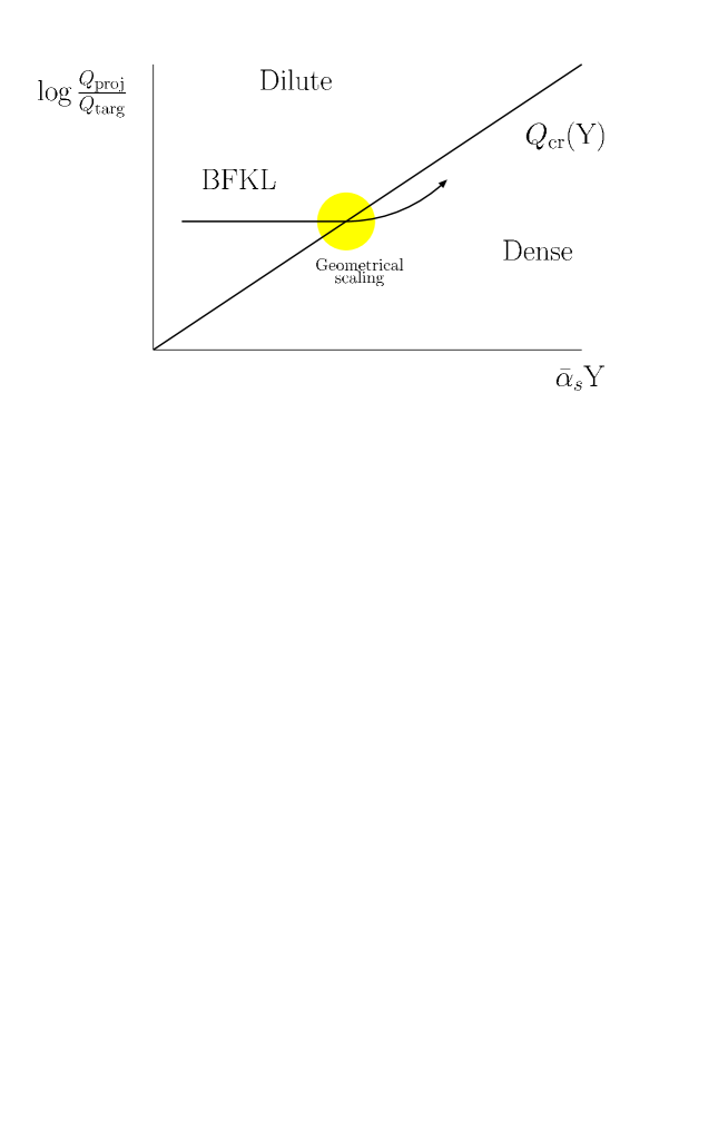
This “saturation line” is represented in Fig. 16. Taking into account Eq. (4.24) it is easy to show that the saturated amplitude in Eq. (4.23) manifests an extra approximate symmetry at . The appearance of scaling symmetries is common in critical phenomena. In our case the BFKL Green’s function with saturation is, up to very mild subleading corrections, invariant under the scaling transformation
| (4.25) |
We can then identify with a critical exponent.
The invariance of scattering amplitudes under this scaling transformation is known as “geometric scaling” in DIS at small and has been experimentally observed in HERA data [33] for the cross sections in the region over a large range in , see Fig. 17.

4.4 Holographic map to critical gravitational collapse
Now that we have described an approach to unitarization in high energy QCD we have all the ingredients needed to propose a holographic map with the formation of a tiny black hole. We identify the region of linear growth with in the QCD side with that of time evolution on a supercritical line just above the critical manifold of codimension one present in our gravitational studies of a perfect fluid (see Fig. 18). We set the initial critical density distribution of perfect fluid at time and evolve the system following Einstein’s and matter equations of motion.
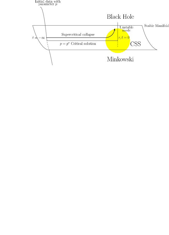
It is also natural to map the radial component in the gravity side to in the gauge theory sector. Both variables measure the spread of the system on a space “orthogonal” to the holographic direction. Note that the typical virtuality should be large enough to ensure a perturbative description of the scattering. This brings us to the region of the critical collapse, precisely the zone where the black hole is formed.
The competition in QCD between Reggeon exchange, which, as we have already explained, tends to reduce the size of the amplitude, and the emission of on–shell gluons, with the opposite effect, has an interpretation during the collapse: it corresponds to the balance between self–gravitational attraction and kinetic energy, or pressure, in the perfect fluid. To understand this correspondence in more detail we can go back to Eq. (4.22) and note that in the unitarized solution the dominant background is . This is a non–trivial statement since now we are not at the minimum of as in the original BFKL case. The dominant region of integration is shifted towards the ultraviolet pole at . This implies that the net effect of non–linear unitarity corrections is to suppress the diffusion towards the infrared region.
This can be mapped into the dual gravitational collapse framework. The infrared modes in QCD have small virtualities and therefore occupy large regions in the transverse plane. The physics of saturation is that of a system with perturbative degrees of freedom forced to grow in a finite region. The critical line in Eq. (4.24) shows that, in order to accommodate further multiplicity, the preferred configurations are those with small transverse size, i.e. large virtualities. This is exactly what happens when the black hole is formed: the largest part of the initial collapsing matter does not confine in a compact size and expands infinitely, while only a minute fraction remains within the tiny black hole radius in the region . It is natural to think that the black hole contains the bulk of collapsing modes with the smallest spread in the radial component.
At asymptotic energies we can heuristically picture the mechanism of suppression of infrared modes as that of a two–dimensional disk packing. It is useful to go back to the linear BFKL equation and notice that the evolution it describes is not sensitive to the transverse size of the gluons in the ladder. This is a consequence of the lack of ordering in transverse scales, which generates an IR/UV symmetric random walk in these variables. In some sense, the system does not have memory of the transverse size of the previous steps in the evolution and is insensitive to the size of the target. Note that , corresponding to the minimum of , is the only –background where the saddle point condition in Eq. (4.19) does not mix longitudinal and transverse components. As it was shown in Eq. (4.5) the gluon Green’s function is the sum of many configurations with different multiplicities.
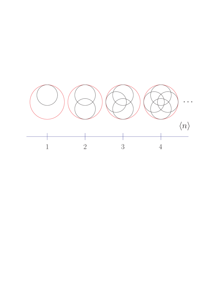
We can then represent the asymptotic linear evolution as a function of the multiplicity in Fig. 19 where the average transverse size of each gluon is represented by the circles, which are allowed to overlap. The largest circle corresponds to the target’s transverse size.
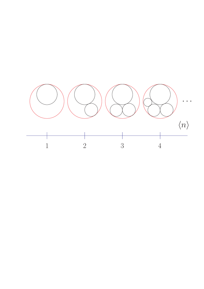
Nearby the saturation line the parton evolution is constrained by the relation in Eq. (4.24) which we can write in terms of transverse sizes as
| (4.26) |
This implies that each gluon decreases its transverse size with respect to the previous one as the energy grows. This introduces ordering in and suppresses the random walks towards lower virtualities enhancing the diffusion into ultraviolet modes. The system can now resolve the transverse size of the target and it can be pictured as a problem of packing many hard disks within a circular boundary without allowing overlapping. This is pictorially shown in Fig. 20. The fact that we have CSS indicates that there is a fractal structure in the evolution since the system reproduces itself at shorter distances.
In terms of the function in Fig. 15 we can associate gravitational potential energy with the term and kinetic energy with . Thus, for kinetic energy dominates, with no formation of a black hole. This corresponds to violation of unitarity in the Yang–Mills side. The threshold for formation of a black hole corresponds to , when the gravitational potential energy is large enough to neutralize its kinetic counterpart. This is interpreted as the existence of a unitarization mechanism in QCD.
Let us indicate again that the QCD transition from linear evolution, which corresponds to a “dilute” region in the transverse space, towards the “dense” regime is characterized by the critical anomalous dimension and the “saturation exponent”, It is remarkable that these are pure numbers independent of any kinematic variable or the ’t Hooft coupling. The interesting phenomena discovered by Choptuik, which we have reproduced here for arbitrary dimension, is that the perfect fluid goes through a similar process at the threshold of formation of the black hole with its radius scaling as
| (4.27) |
with some fiducial length scale. The exponent is also a pure number which depends on the dimension and the speed of sound in the fluid, . It is difficult to find compelling holographic arguments to select a particular value of . Nevertheless, we believe that the limit of “radiation fluid” is the correct one. In this case and the energy–momentum tensor is traceless. This would support our intuition that a conformal symmetry underlies the crossover region towards the black hole formation. We find further evidence in this direction when we look at Table 1 and see that the values for in the radiation fluid case are 2.58, 2.48 and 2.42 in dimensions five, six and seven, respectively. These values are very similar to in the gauge theory side.
At the stage we are in our holographic analysis it is not possible to precisely determine in which dimension the dual gravitational physics must live. From the previous arguments it seems it should not be far from dimension four. In a previous analysis [1] it was argued that the mapping could be to dimension five. This was based on the study of spherically symmetric collapse of a massless scalar field [7]. There, a relation identical to (4.27) was found for the size of the tiny black hole formed when imploding an initial radial density of static scalar field. It turns out that in this case is very similar to in QCD when the scalar field propagates in five dimensions. As discussed in the Introduction, the collapse of a scalar field also manifests discrete self–similarity. This means that the metric and field components at the critical manifold, generally denoted by , reproduce themselves after a finite echoing period . This means that , where in five dimensions [5]. However, it turns out that there is no analogue of this echoing period in the Yang–Mills theory side.
As we already have discussed, in the case of a spherical collapse of a perfect fluid with equation of state , there is also self-similarity but in this case it is continuous (CSS). This implies that we can write the critical solution as a function of the variable defined in Eq. (2.14) only, i.e. .
In Section 2 we found the critical CSS solution by solving the Einstein equations sourced by a perfect fluid. As an example in four dimensions, we can look at the profile of the function which is proportional to the ratio of the mean density inside the sphere of radius to the local density at . In Fig. 21 we show how maintains a constant –profile for different values of . This implies that the solution is CSS since any continuous change in the time coordinate can be compensated by a change in leaving the solution invariant. The mapping of this scaling symmetry in the QCD side corresponds to the dual geometrical scaling in Eq. (4.25).
It is important to note that in QCD geometric scaling is only present in the region very close to the saturation line. In the same way the CSS present in the gravitational critical solution breaks down very rapidly when we introduce a Liapunov perturbation of the form shown in Eq. (3.1).
The Choptuik exponent characterizing the black hole radius of Eq. (4.27) can be obtained by searching for these Liapunov modes of instability of the CSS solution. In Fig. 22 we show how the exponentially growing mode removes CSS from the solution to the collapse. The rate of growth of this mode is given by a coefficient which coincides with the Choptuik exponent. As explained in previous Sections, we have numerically extracted this coefficient in different dimensions.
To summarize this Section, in QCD there exist two interesting types of nonperturbative physics: one is the confinement/deconfinement phase transition with a gravity dual [35] given by a Hawking-Page type of phase transitions [34]. The other one, stressed in this article, is the phenomena of parton saturation or dilute/dense system of partons transition which we suggest to have its gravity dual in the critical formation of tiny black holes. Whereas in the confinement/deconfinement phase transition in Hawking-Page representation we have an entropic balance to characterize black hole nucleation, in the parton saturation case we have an infrared–ultraviolet energy competition which we map into a potential/kinetic energy competition in the gravity dual.


5 Unanswered questions and work in progress
We are aware of the fact that we are exploring unchartered territory. On the gravitational side we are looking at the formation of small black holes, with the corresponding high curvatures and hence the need to introduce corrections in in the Einstein equations of motion. We try to relate holographically this region with a yet not fully understood region in QCD or Yang-Mills theory: the realm of the hard Pomeron. Some rudiments of the would-be correspondence have been spelt out in the previous Section. We list here a number of open questions, general philosophy, and work in progress.
So far we have considered the collapse of either scalar fields or perfect fluids. The next step is to consider gravitational collapse in the case of a full type-IIB string theory. We are currently working on this problem, and there are some interesting provisos worth discussing. First the beta-function equations in type-IIB receive corrections starting at four-loop order in , hence if we do not consider curvatures close to the string length our arguments should be reliable at least qualitatively. Within the spirit of Choptuik computations, since we are considering the formation of very small black holes, the cosmological constant should not be relevant in the computation of the Choptuik exponents. What is not clear however, is whether we are forming small five-dimesional AdS black holes [34] or a small ten-dimensional Schwarzschild black holes embedded in AdSS5, a possibility shown in [36]. The Choptuik exponent is likely to depend on the various scenarios. This is currently being investigated, and we hope to report our results in the future [37].
In all our computations, supersymmetry does not seem to play any rôle. It is important to stress that the viability of the proposed holographic relation lies in the fact that we are computing critical exponents, normally protected by some form of universality. This is the only stability protection we can advocate against all corrections imaginable. In addition, on the gauge theory side we have an effective large- expansion generated by the BFKL analysis. Their effective is proportional to . To what extent this leads to a systematic “large-” expansion remains to be seen, but should such an expansion exist it would also provide some substance to our musings.
The region we are trying to explore, at least on the gauge theory side is accessible to experiment. How the BFKL evolution is unitarized remains to be understood. Our claim is that under a holographic map this should give precious clues on how gravitational collapse becomes “unitarized” before forming a singularity. On the QCD side the BFKL evolution is thought to lead to the color glass condensate [31] (for a review see [38]) or some similar scenario in which we go from a single reggeized particle to a many-body state. This mechanism is somewhat reminiscent of the Klein paradox.
In string theory [39], it is possible to give a heuristic description of how, as we approach the formation of the horizon in gravitational collapse, the description in terms of a “single” string should evolve into a multi-string system, thus diluting the formation of a singularity. This analysis is based on entropy arguments, and for the time being we do not know how to holographically match these arguments with an entropic argument in the CGC. The formation of the latter, as well as the scaling arguments in gravitational collapse are deeply dynamical phenomena, far from any notion of equilibrium. At this moment it does not seem easy to make a connection between both arguments. We believe, however, that the formation of the CGC (or whatever unitarizes the BFKL evolution) will, through a holographic map, provide a description of what happens in the final stages of gravitational collapse. If this picture is right, the exploration of the Regge region in future colliders is likely to give us a completely new panorama of what happens when black holes form.
Acknowledgments
We have benefited from discussions and criticisms from many colleagues. We would like to thank J. L. F. Barbón, J. Bartels, D. Berenstein, M. Choptuik, M. Ciafaloni, L. Cornalba, J. Edelstein, R. Emparan, D. Gross, H. Itoyama, B. Kol, A. Kumar, G. Kunstatter, K. Kunze, L. Lipatov, H. Liu, M. Mariño, J. M. Martín-García, D. Mateos, T. Ortín, F. Schaposnik, M. M. Sheikh-Jabbari, and S. Wadia for comments and discussion which helped sharpen our ideas and presentation. The work of C.G. has been partially supported by the Spanish DGI contract FPA2003-02877 and the CAM grant HEPHACOS P-ESP-00346. A.T. thanks the Marie Curie and the Freydoon Mansouri foundations for support, and the CERN Theory Group for hospitality. M.A.V.-M. acknowledges partial support from the Spanish Government Grants PA2005-04823, FIS2006-05319 and Spanish Consolider-Ingenio 2010 Programme CPAN (CSD2007-00042), and thanks the CERN Theory Group for hospitality.
Appendix A. The Einstein equations
In this Appendix we detail the derivation of the Einstein equations for the line element
| (A.1) |
coupled to a perfect-fluid energy-momentum tensor (2.2). Here is the line element for a -dimensional space of constant curvature . The case with corresponds to the spherically symmetric case studied in this paper.
In order to write the geometric side of the Einstein equations it is very convenient to introduce a system of tetrads
| (A.2) |
where is a system of tetrads for the transverse space satisfying .
The Riemannnian spin connection can be computed from the torsion-free conditions , with the result
| (A.3) |
with the spin connection for the constant curvature transverse space, satisfying . The nonvanishing components of curvature form are given by
| (A.4) | |||||
where is the curvature form of the constant curvature space
| (A.5) |
The components of the Ricci tensor in the tetrad frame can be read from this expressions using
| (A.6) |
Then the Einstein tensor in the orthonormal frame , with , is given by
| (A.7) | |||||
The next step is to compute the right-hand side of the Einstein equations. Again we work in the tetrad frame where the four-velocity is given by
| (A.8) |
so the energy-momentum tensor has the simple form . With this we can write the full set of Einstein equations . For the sake of simplicity, however, it is convenient to replace the more complicated components by the Bianchi identities (2.5). For the 00, 01 and 11 component of the Einstein equations one arrives after simple algebraic manipulations to Eqs. (2.4).
Appendix B. Calculation of the coefficients in Eq. (2.27)
In this Appendix we outline the procedure to compute the second coefficients of the expansion of as a series expansion in powers of . Taking a derivative with respect to in the last equation in (2.22) and defining the right-hand side of the expression using the l’Hôpital rule we arrive at
| (B.1) |
where by we denote the numerator of the right-hand side of the last equation in (2.22)
| (B.2) |
At the sonic point this satisfies
As we have already argued, all derivatives at the sonic point should be a function of just one parameter that we can take to be . Indeed, all the derivatives appearing in Eq. ( ‣ Appendix B. Calculation of the coefficients in Eq. (2.27)) can be written in terms of and by using
| (B.4) | |||||
together with
| (B.5) |
and
| (B.6) | |||||
In addition, Eq. (2.50) with the choice of the minus branch is also needed.
Plugging all these expressions into Eq. (B.1) we arrive at a linear equation for that determines also . The fact that this equation is linear is of conceptual importance. It means that, fixed the ambiguity in the choice of the branch determining there is no further ambiguity in the calculation of . In fact, this extends to the calculation of all higher derivatives. The algebraic equations giving the values of the -th derivative at the sonic point are always linear.
Appendix C. Some details of the calculation of perturbations
In this Appendix we give the expressions for the derivatives of the coefficients needed to solve the perturbation equations around the singular points. In order to evaluate (3.16) the following derivatives are required
| (C.1) | |||||
In addition, the derivatives of , and are also needed. For the first two we have
| (C.2) |
whereas can be written as
| (C.3) |
where and are given respectively by
References
-
[1]
L. Álvarez-Gaumé, C. Gómez and M. A. Vázquez-Mozo,
Scaling Phenomena in Gravity from QCD,
Phys. Lett. B649 (2007) 478
[arXiv:hep-th/0611312].
L. Álvarez-Gaumé, C. Gómez, A. Sabio Vera, A. Tavanfar and M. A. Vázquez-Mozo, Gluon Saturation and Black Hole Criticality, in “Forward Physics and QCD”, eds. J. Bartels, K. Borras, M. Diehl and H. Jung, DESY 2007. arXiv:0710.2517 [hep-th]. - [2] R. C. Brower, J. Polchinski, M. J. Strassler and C. I. Tan, The Pomeron and Gauge/String Duality, J. High Energy Phys. 12 (2007) 005 [arXiv:hep-th/0603115].
- [3] Y. Hatta, E. Iancu and A. H. Mueller, Deep inelastic scattering at strong coupling from gauge/string duality: the saturation line, J. High Energy Phys. 01 (2008) 026 [arXiv:0710.2148 [hep-th]].
-
[4]
R. C. Brower, S. D. Mathur and C. I. Tan,
From black holes to pomeron: Tensor glueball and pomeron intercept at
strong coupling, in: “QCD and multiparticle production”, Eds. I. Sarcevic and
C. I. Tan, World Scientific 2000
[arXiv:hep-ph/0003153].
R. A. Janik, String fluctuations, AdS/CFT and the soft pomeron intercept, Phys. Lett. B500 (2001) 118 [arXiv:hep-th/0010069].
C. I. Tan, Pomeron and AdS/CFT correspondence for QCD, in: “From to heavy ion collisions”, Eds. T. Csorgo, S. Hegyi and W. Kittel, World Scientific 2001 [arXiv:hep-ph/0102127].
R. C. Brower and C. I. Tan, QCD hard scattering from string/gauge duality, Nucl. Phys. Proc. Suppl. 119 (2003) 938.
C. I. Tan, String/gauge duality and soft-hard pomeron, Acta Phys. Polon. B 36 (2005) 711.
L. Cornalba, M. S. Costa and J. Penedones, Eikonal Methods in AdS/CFT: BFKL Pomeron at Weak Coupling, arXiv:0801.3002 [hep-th]. -
[5]
E. Sorkin and Y. Oren,
On Choptuik’s scaling in higher dimensions,
Phys. Rev. D71 (2005) 124005
[arXiv:hep-th/0502034].
J. Bland, B. Preston, M. Becker, G. Kunstatter and V. Husain, Dimension dependence of the critical exponent in spherically symmetric gravitational collapse, Class. Quant. Grav. 22 (2005) 5355.
J. Bland and G. Kunstatter, The 5-D Choptuik critical exponent and holography, Phys. Rev. D75 (2007) 101501 [arXiv:hep-th/0702226]. -
[6]
C. Gundlach,
Critical phenomena in gravitational collapse,
Phys. Rept. 376 (2003) 339
[arXiv:gr-qc/0210101].
C. Gundlach and J. M. Martín-García, Critical phenomena in gravitational collapse, Living Rev. Rel. 2 (1999) 4 [arXiv:0711.4620 [gr-qc]]. - [7] M. W. Choptuik, Universality And Scaling In Gravitational Collapse Of A Massless Scalar Field, Phys. Rev. Lett. 70 (1993) 9.
- [8] C. R. Evans and J. S. Coleman, Observation of critical phenomena and selfsimilarity in the gravitational collapse of radiation fluid, Phys. Rev. Lett. 72 (1994) 1782 [arXiv:gr-qc/9402041].
- [9] B. J. Carr and A. A. Coley, Self-Similarity in General Relativity Class. Quant. Grav. 16 (1999) R31 [arXiv:gr-qc/9806048].
-
[10]
T. Koike, T. Hara and S. Adachi,
Critical behavior in gravitational collapse of radiation fluid: A
Renormalization group (linear perturbation) analysis,
Phys. Rev. Lett. 74 (1995) 5170
[arXiv:gr-qc/9503007].
T. Koike, T. Hara and S. Adachi, Critical behavior in gravitational collapse of a perfect fluid, Phys. Rev. D59 (1999) 104008.
T. Hara, T. Koike and S. Adachi, Renormalization group and critical behaviour in gravitational collapse, arXiv:gr-qc/9607010. - [11] T. Harada and H. Maeda, Convergence to a self-similar solution in general relativistic gravitational collapse, Phys. Rev. D63 (2001) 084022 [arXiv:gr-qc/0101064].
- [12] A. Ori and T. Piran, Naked Singularities and Other Features of Selfsimilar General Relativistic Gravitational Collapse, Phys. Rev. D42 (1990) 1068.
- [13] C. Hunter, The collapse of unstable isothermal spheres, Astrophys. J. 218 (1977) 834.
-
[14]
V. S. Fadin, E. A. Kuraev and L. N. Lipatov,
On The Pomeranchuk Singularity In Asymptotically Free Theories,
Phys. Lett. B60 (1975) 50.
E. A. Kuraev, L. N. Lipatov and V. S. Fadin, Multi - Reggeon Processes In The Yang-Mills Theory, Sov. Phys. JETP 44 (1976) 443
L. N. Lipatov, Reggeization Of The Vector Meson And The Vacuum Singularity In Nonabelian Gauge Theories, Sov. J. Nucl. Phys. 23 (1976) 338
E. A. Kuraev, L. N. Lipatov and V. S. Fadin, The Pomeranchuk Singularity In Nonabelian Gauge Theories, Sov. Phys. JETP 45 (1977) 199
I. I. Balitsky and L. N. Lipatov, The Pomeranchuk Singularity In Quantum Chromodynamics, Sov. J. Nucl. Phys. 28 (1978) 822 -
[15]
I. Balitsky,
Operator expansion for high-energy scattering,
Nucl. Phys. B463 (1996) 99
[arXiv:hep-ph/9509348].
Y. V. Kovchegov, Small-x structure function of a nucleus including multiple pomeron exchanges,’ Phys. Rev. D60 (1999) 034008 [arXiv:hep-ph/9901281]. - [16] L. Álvarez-Gaumé, C. Gómez, A. Sabio Vera, A. Tavanfar and M. A. Vázquez-Mozo, in progress.
-
[17]
G. V. Bicknell and R. N. Henriksen, Self-similar growth of primordial black holes. I - Stiff equation
of state, Astrophys. J. 219 (1978) 1043.
G. V. Bicknell and R. N. Henriksen, Self-similar growth of primordial black holes. II - General sound speed, Astrophys. J. 225 (1978) 237. -
[18]
J. R. Forshaw and D. A. Ross, Quantum Chromodynamics and the Pomeron,
Cambridge 1997.
S. Donnachie, G. Dosch, P. Landshoff and O. Nachtmann, Pomeron Physics and QCD, Cambridge 2002.
V. Barone and E. Pedrazzi, High-Energy Particle Diffraction, Springer 2002. - [19] J. M. Maldacena, The large N limit of superconformal field theories and supergravity, Adv. Theor. Math. Phys. 2 (1998) 231 [arXiv:hep-th/9711200].
-
[20]
S. S. Gubser, I. R. Klebanov and A. M. Polyakov,
Gauge theory correlators from non-critical string theory,
Phys. Lett. B428 (1998) 105
[arXiv:hep-th/9802109].
E. Witten, Anti-de Sitter space and holography, Adv. Theor. Math. Phys. 2 (1998) 253 [arXiv:hep-th/9802150].
O. Aharony, S. S. Gubser, J. M. Maldacena, H. Ooguri and Y. Oz, Large N field theories, string theory and gravity, Phys. Rept. 323 (2000) 183 [arXiv:hep-th/9905111]. - [21] G. S. Danilov and L. N. Lipatov, BFKL pomeron in string models, Nucl. Phys. B754 (2006) 187 [arXiv:hep-ph/0603073].
- [22] A. V. Kotikov, L. N. Lipatov, A. I. Onishchenko and V. N. Velizhanin, Three-loop universal anomalous dimension of the Wilson operators in SUSY Yang-Mills model, Phys. Lett. B 595 (2004) 521 [Erratum-ibid. B 632 (2006) 754] [arXiv:hep-th/0404092].
- [23] J. Bartels and H. Kowalski, Diffraction at HERA and the confinement problem, Eur. Phys. J. C19 (2001) 693 [arXiv:hep-ph/0010345].
-
[24]
V. N. Gribov and L. N. Lipatov,
Deep Inelastic E P Scattering In Perturbation Theory,
Sov. J. Nucl. Phys. 15 (1972) 438
V. N. Gribov and L. N. Lipatov, Pair Annihilation And Deep Inelastic e-p Scattering In Perturbation Theory, Sov. J. Nucl. Phys. 15 (1972) 675 [Yad. Fiz. 15 (1972) 1218].
L. N. Lipatov, The parton model and perturbation theory, Sov. J. Nucl. Phys. 20 (1975) 94
G. Altarelli and G. Parisi, Asymptotic Freedom in Parton Language, Nucl. Phys. B126 (1977) 298.
Y. L. Dokshitzer, Calculation of the Structure Functions for Deep Inelastic Scattering and Annihilation by Perturbation Theory in Quantum Chromodynamics. Sov. Phys. JETP 46 (1977) 641 -
[25]
H. Liu, K. Rajagopal and U. A. Wiedemann,
Calculating the jet quenching parameter from AdS/CFT,
Phys. Rev. Lett. 97 (2006) 182301
[arXiv:hep-ph/0605178].
H. Liu, K. Rajagopal and U. A. Wiedemann, An AdS/CFT calculation of screening in a hot wind, Phys. Rev. Lett. 98 (2007) 182301 [arXiv:hep-ph/0607062].
H. Liu, K. Rajagopal and U. A. Wiedemann, Wilson loops in heavy ion collisions and their calculation in AdS/CFT, J. High Energy Phys. 03 (2007) 066 [arXiv:hep-ph/0612168]. - [26] J. Polchinski and M. J. Strassler, Deep inelastic scattering and gauge/string duality, J. High Energy Phys. 05 (2003) 012 [arXiv:hep-th/0209211].
-
[27]
A. V. Kotikov and L. N. Lipatov,
NLO corrections to the BFKL equation in QCD and in supersymmetric gauge
theories,
Nucl. Phys. B582 (2000) 19
[arXiv:hep-ph/0004008].
J. R. Andersen and A. Sabio Vera, The gluon Green’s function in supersymmetric Yang-Mills theory, Nucl. Phys. B699 (2004) 90 [arXiv:hep-th/0406009].
V. S. Fadin and R. Fiore, The dipole form of the BFKL kernel in supersymmetric Yang–Mills theories, Phys. Lett. B661 (2008) 139 [arXiv:0712.3901 [hep-ph]]. -
[28]
J. Bartels, L. N. Lipatov and A. Sabio Vera,
BFKL Pomeron, Reggeized gluons and Bern-Dixon-Smirnov amplitudes,
arXiv:0802.2065 [hep-th].
V. Del Duca and E. W. N. Glover, Testing high-energy factorization beyond the next-to-leading-logarithmic accuracy, arXiv:0802.4445 [hep-th]. - [29] J. Bartels, L. N. Lipatov and M. Wüsthoff, Conformal Invariance of the Transition Vertex gluons, Nucl. Phys. B 464 (1996) 298 [arXiv:hep-ph/9509303].
- [30] L. N. Lipatov, The Bare Pomeron In Quantum Chromodynamics, Sov. Phys. JETP 63 (1986) 904
-
[31]
E. Iancu, A. Leonidov and L. D. McLerran,
Nonlinear gluon evolution in the color glass condensate. I,
Nucl. Phys. A692 (2001) 583
[arXiv:hep-ph/0011241].
E. Iancu, A. Leonidov and L. D. McLerran, The renormalization group equation for the color glass condensate, Phys. Lett. B510 (2001) 133 [arXiv:hep-ph/0102009]. -
[32]
L. V. Gribov, E. M. Levin and M. G. Ryskin,
Semihard Processes In QCD,
Phys. Rept. 100 (1983) 1.
A. H. Mueller and D. N. Triantafyllopoulos, The energy dependence of the saturation momentum, Nucl. Phys. B640 (2002) 331 [arXiv:hep-ph/0205167]. - [33] A. M. Staśto, K. J. Golec-Biernat and J. Kwieciński, Geometric scaling for the total p cross-section in the low-x region, Phys. Rev. Lett. 86 (2001) 596 [arXiv:hep-ph/0007192].
- [34] S. W. Hawking and D. N. Page, Thermodynamics Of Black Holes In Anti-De Sitter Space, Commun. Math. Phys. 87 (1983) 577.
- [35] E. Witten, Anti-de Sitter space, thermal phase transition, and confinement in gauge theories, Adv. Theor. Math. Phys. 2 (1998) 505 [arXiv:hep-th/9803131].
-
[36]
G. T. Horowitz and V. E. Hubeny,
Note on small black holes in ,
J. High Energy. Phys. 06 (2000) 031
[arXiv:hep-th/0005288].
G. T. Horowitz and V. E. Hubeny, CFT description of small objects in AdS, J. High Energy Phys. 10 (2000) 027 [arXiv:hep-th/0009051]. - [37] L. Álvarez-Gaumé, C. Gómez, A. Sabio Vera, A. Tavanfar and M. A. Vázquez-Mozo, in progress.
-
[38]
E. Iancu, A. Leonidov and L. McLerran,
The colour glass condensate: An introduction, in “QCD perspectives on hot and dense
matter”, Eds. J.-P. Blaizot and E. Iancu, Kluwer 2002
[arXiv:hep-ph/0202270].
E. Iancu and R. Venugopalan, The color glass condensate and high energy scattering in QCD, in: “Quark-Gluon Plasma 3”, Eds. R. C. Hwa and X. N. Wang, World Scientific 2004 [arXiv:hep-ph/0303204]. -
[39]
L. Susskind,
Some speculations about black hole entropy in string theory,
in “The Black Hole: 25 Years After”, eds. C. Teitelboim and J. Zanelli, World Scientific 1998
[arXiv:hep-th/9309145].
G. T. Horowitz and J. Polchinski, A correspondence principle for black holes and strings, Phys. Rev. D55 (1997) 6189 [arXiv:hep-th/9612146].
G. T. Horowitz and J. Polchinski, Self gravitating fundamental strings, Phys. Rev. D57 (1998) 2557 [arXiv:hep-th/9707170].
T. Damour and G. Veneziano, Self-gravitating fundamental strings and black holes, Nucl. Phys. B 568 (2000) 93 [arXiv:hep-th/9907030].