Steady-state Lévy flights in a confined domain

Abstract

We derive the generalized Fokker-Planck equation associated with a Langevin equation driven by arbitrary additive white noise. We apply our result to study the distribution of symmetric and asymmetric Lévy flights in an infinitely deep potential well. The fractional Fokker-Planck equation for Lévy flights is derived and solved analytically in the steady state. It is shown that Lévy flights are distributed according to the beta distribution, whose probability density becomes singular at the boundaries of the well. The origin of the preferred concentration of flying objects near the boundaries in nonequilibrium systems is clarified.

I INTRODUCTION

It is remarkable, and at first sight surprising, that a large variety of physical, biological, financial, and other processes can be described by stable Lévy processes with infinite variance 1 ; 2 ; 3 . The latter are defined as continuous-time random processes whose independent and stationary increments are distributed according to heavy-tailed stable distributions. The main feature of these distributions is that the tails cannot be cut off or, in other words, rare but large events cannot be neglected. As a consequence, the classical stochastic theory, which is based on the ordinary central limit theorem, is no longer valid.

Due to the heavy-tailed distributions of the increments, stable Lévy processes exhibit large jumps, and for this reason these processes are often called Lévy flights. Lévy flights are actually observed in various real systems. Representative examples include, for instance, fluorescent probes in living polymers OBLU , tracer particles in rotating flows SWS , ions in optical lattices KSW , cooled atoms in laser fields BBAC , subsurface hydrology 8 ; 9 , and ecology 10 ; 11 ; 12 , though a recent work questions the empirical evidence for Lévy flights in animal search patterns EdPhWaFrMu07 . Lévy flights have also been predicted for a large number of model systems 1 ; 2 ; 3 . The ubiquity of these processes is supported by the generalized central limit theorem GK , which states that all limiting distributions of properly normalized and centered sums of independent, identically distributed random variables are stable.

The Langevin equation is one of the most important tools for studying noise phenomena in systems coupled to a fluctuating environment. Introduced by Paul Langevin just one hundred years ago Lang to describe the dynamics of a Brownian particle, this equation and its various modifications are widely used in many areas of science CKW . The Langevin equation driven by Lévy white noise, i.e., noise defined as a time derivative, in the sense of generalized functions, of a stable Lévy process, provides a basis for the study of Lévy flights in external potentials. It has been shown that the probability density of Lévy flights satisfies the fractional Fokker-Planck (FP) equation 17 ; 18 ; 19 ; 20 ; 21 . The steady-state solutions of this equation describing confined Lévy flights, i.e., flights with finite variance, are of particular interest. One reason is that these solutions will clarify the distribution of flying objects in confined domains. This is an important issue, especially near impermeable boundaries, in such complex systems as confined plasmas and turbulent flows. Another reason is that exact general solutions of a simple form, which are valid for any Lévy white noise, will be very useful for testing a variety of numerical methods in this area 22 ; 23 ; 24 . However, known solutions are related to power potentials and to a very special case of Lévy white noise with unit index of stability and zero skewness parameter 25 ; 26 , and thus they are not suitable for those purposes.

It should be noted that Lévy white noises do not exhaust all possible white noises. As a consequence, the fractional FP equation is a particular case of the generalized FP equation, which corresponds to the Langevin equation driven by an arbitrary white noise. Since any white noise is defined as a time derivative, in the sense of generalized functions, of a stationary process with independent increments, it can be characterized by the transition probability density or, alternatively, by the characteristic function of this white noise generating process. One expects therefore that the term in the generalized FP equation that describes the effect of the noise on the dynamics of the system can also be expressed via the characteristic function. The derivation of the generalized FP equation is of great importance because it accounts for all possible white noise effects in a unified way and will be very useful for applications.

In this paper, we put forward the generalized FP equation and find the analytical solution of this equation for steady-state Lévy flights in a confined geometry.

II GENERALIZED FOKKER-PLANCK EQUATION

In many applications, ranging from physical and chemical to biological and social systems, the relevant degrees of freedom of these systems obey a (dimensionless) Langevin equation that is equivalent to the equation of motion for an overdamped particle

$$\dot{x}(t)=f(x(t),t)+\xi(t).$$ (1)

Here, $x(t)$ is a particle coordinate, $x(0)=0$, $f(x,t)=-\partial U(x,t)/\partial x$ is a force field, $U(x,t)$ is an external deterministic potential, and $\xi(t)$ is a random force (noise) resulting from a fluctuating environment. Though the quantities in Eq. (1) have different meanings for different systems, we will use the above terminology to be concrete.

Under certain conditions (see, e.g., Refs. HL ; HJ ), the noise $\xi(t)$ can be chosen to be white. In this case, the increment $\delta x(t)=x(t+\tau)-x(t)$ of the particle coordinate during a time interval $\tau$ ($\tau\to 0$) is written as

$$\delta x(t)=f(x(t),t)\tau+\delta\eta(t),$$ (2)

which defines the meaning of Eq. (1) in the white-noise approximation. Here $\delta\eta(t)=\eta(t+\tau)-\eta(t)=\int_{t}^{t+\tau}dt^{\prime}\xi(t^{\prime})$, and we assume that the integral exists in the mean square sense. A white noise generating process, i.e., a stationary random process $\eta(t)=\lim_{\tau\to 0}\sum_{j=0}^{[t/\tau]-1}\delta\eta(j\tau)$, with $\eta(0)=0$ and where $[t/\tau]$ denotes the integer part of $t/\tau$, is completely defined by the transition probability density $p(\eta_{j+1},\tau|\eta_{j})$ of a discrete-time process $\eta(n\tau)=\sum_{j=0}^{n-1}\delta\eta(j\tau)$ ($n\geq 1$) as $\tau\to 0$. Here $\eta_{j+1}$ and $\eta_{j}$ denote the possible values of $\eta(j\tau+\tau)$ and $\eta(j\tau)$, respectively. Note that all transition probability densities of the form $p(\eta_{j+k},k\tau|\eta_{j})$ can be expressed through $p(\eta_{j+1},\tau|\eta_{j})$ by using the Chapman-Kolmogorov equation HL ; V-K ; HT . In particular, $p(\eta_{j+2},2\tau|\eta_{j})=\int d\eta_{j+1}p(\eta_{j+2},\tau|\eta_{j+1})p(\eta_{j+1},\tau|\eta_{j})$. This implies that the influence of any white noise on the system can also be fully characterized by the function $p(\eta_{j+1},\tau|\eta_{j})$. We assume that the transition probability density $p(\eta_{j+1},\tau|\eta_{j})$ is properly normalized, $\int_{-\infty}^{\infty}d\eta_{j+1}p(\eta_{j+1},\tau|\eta_{j})=1$, and that it satisfies the condition $\lim_{\tau\to 0}p(\eta_{j+1},\tau|\eta_{j})=\delta(\eta_{j+1}-\eta_{j})$, where $\delta(\cdot)$ stands for the Dirac $\delta$ function. For simplicity, we also assume that $p(\eta_{j+1},\tau|\eta_{j})=p(\Delta\eta,\tau)$ with $\Delta\eta=\eta_{j+1}-\eta_{j}$.

We define the probability density of the particle coordinate $x(t)$ in the usual way, namely $P(x,t)=\langle\delta(x-x(t))\rangle$, where the angular brackets denote averaging over the noise. Taking the Fourier transform of $P(x,t)$ according to the definition $\mathcal{F}\{g(x)\}\equiv g_{k}=\int_{-\infty}^{\infty}dx\,e^{-ikx}g(x)$, we obtain $P_{k}(t)=\langle e^{-ikx(t)}\rangle$, i.e., the characteristic function of $x(t)$. Equation (2) implies that the increment of this quantity, $\delta P_{k}=P_{k}(t+\tau)-P_{k}(t)$, can be written in the form $\delta P_{k}=-ik\tau\langle e^{-ikx(t)}f(x(t),t)\rangle+\langle e^{-ikx(t)}(e^{-ik\delta\eta(t)}-1)\rangle$ as $\tau\to 0$. The use of the well-known properties of the Fourier transform yields $ik\langle e^{-ikx(t)}f(x(t),t)\rangle=\mathcal{F}\{\partial f(x,t)P(x,t)/\partial x\}$, and the statistical independence of $x(t)$ and $\delta\eta(t)$ implies DVH $\langle e^{-ikx(t)}(e^{-ik\delta\eta(t)}-1)\rangle=P_{k}(t)(p_{k}(\tau)-1)$, where $p_{k}(\tau)=\mathcal{F}\{p(\Delta\eta,\tau)\}=\langle e^{-ik\delta\eta(t)}\rangle$ is the characteristic function of $\delta\eta(t)$. Dividing $\delta P_{k}$ by $\tau$ and taking the limit $\tau\to 0$, we obtain the generalized FP equation in Fourier space,

$$\frac{\partial}{\partial t}P_{k}(t)=-\mathcal{F}\Big{\{}\frac{\partial}{\partial x}f(x,t)P(x,t)\Big{\}}+P_{k}(t)\phi_{k},$$ (3)

where $\phi_{k}=\lim_{\tau\to 0}(p_{k}(\tau)-1)/\tau$.

It is advantageous to introduce the characteristic function $S_{k}=\langle e^{-ik\eta(1)}\rangle$ of $\eta(1)$. We rewrite it as $S_{k}=\lim_{\tau\to 0}(p_{k}(\tau))^{[1/\tau]}$, using the formula $\eta(1)=\lim_{\tau\to 0}\sum_{j=0}^{[1/\tau]-1}\delta\eta(j\tau)$. Replacing $p_{k}(\tau)$ by $1+\tau\phi_{k}$ and taking into account that $\lim_{\varepsilon\to 0}(1+\varepsilon)^{1/\varepsilon}=e$, we readily find that $S_{k}=e^{\phi_{k}}$. Finally, applying the inverse Fourier transform $\mathcal{F}^{-1}\{g_{k}\}\equiv g(x)=(1/2\pi)\int_{-\infty}^{\infty}dk\,e^{ikx}g_{k}$ to Eq. (3) and using $\phi_{k}=\ln S_{k}$, we obtain the generalized FP equation in real space

$$\frac{\partial}{\partial t}P(x,t)=-\frac{\partial}{\partial x}f(x,t)P(x,t)+\mathcal{F}^{-1}\{P_{k}(t)\ln S_{k}\},$$ (4)

with $P(x,0)=\delta(x)$, which corresponds to the Langevin equation (1) driven by an arbitrary white noise.

Equation (4) represents our first main result. It constitutes a closed, concise representation of the combination of the Fokker-Planck and Kolmogorov-Feller equations, which are the basic equations governing continuous and discontinuous Markov processes, respectively HL ; V-K ; HT . A remarkable feature of this equation is that it accounts for the noise influence in a unified way, namely by means of the characteristic function $S_{k}$ of the white noise generating process $\eta(t)$ at $t=1$. All presently known FP equations associated with Eq. (1) can be obtained directly from Eq. (4). In particular, if $\xi(t)$ is Poisson white noise characterized by the transition probability density $p(\Delta\eta,\tau)=(1-\lambda\tau)\,\delta(\Delta\eta)+\lambda\tau q(\Delta\eta)$, where $\lambda$ is the average number of jumps of $\eta(t)$ per unit time and $q(\Delta\eta)$ is the probability density of jump sizes, then $S_{k}=e^{-\lambda(1-q_{k})}$ and Eq. (4) yields 32 ; 33 ; 34

$$\frac{\partial}{\partial t}P(x,t)\!\! = \!\!-\frac{\partial}{\partial x}f(x,t)P(x,t)-\lambda P(x,t)$$ (5)

$$\!\!+\lambda\int_{-\infty}^{\infty}dyP(y,t)\,q(x-y).$$

If $\xi(t)$ is Lévy white noise then the generalized central limit theorem GK implies that $S_{k}$ is the characteristic function of Lévy stable distributions. As is well known (see, e.g., Ref. Zol ), the characteristic function $S_{k}(\alpha,\beta,\gamma,\rho)$ of non-degenerate stable distributions depends on four parameters: an index of stability $\alpha\in(0,2]$, a skewness parameter $\beta\in[-1,1]$, a scale parameter $\gamma\in(0,\infty)$, and a location parameter $\rho\in(-\infty,\infty)$. Assuming in accordance with the initial condition $P(x,0)=\delta(x)$ that $\rho=0$ and excluding from consideration the singular case where $\alpha=1$ and $\beta\neq 0$ simultaneously (in this case $\lvert\phi_{k}\rvert=\infty$, and the system reaches the final state immediately), we obtain $S_{k}=S_{k}(\alpha,\beta,\gamma)$, where Zol

$$S_{k}(\alpha,\beta,\gamma)=\exp{\left[-\gamma\lvert k\rvert^{\alpha}\left(1+i\beta\,\text{sgn}(k)\tan\frac{\pi\alpha}{2}\right)\right]}.$$ (6)

Equation (4) with $S_{k}=S_{k}(\alpha,\beta,\gamma)$ can be easily rewritten as a fractional differential equation. The Riemann-Liouville derivatives of a function $g(x)$ on the interval $[-s,s]$ are defined as SKM

$${}_{s}D_{\pm}^{\sigma}g(x)=\frac{(\pm 1)^{n}}{\Gamma(n-\sigma)}\frac{d^{n}}{dx^{n}}\int_{0}^{s\pm x}dy\,g(x\mp y)\,y^{n-\sigma-1}.$$ (7)

Here, ${}_{s}D_{+}^{\sigma}$ and ${}_{s}D_{-}^{\sigma}$ denote the operators of the left- and right-hand side derivatives of order $\sigma$ ($0<\sigma<\infty$), respectively, with $n=1+[\sigma]$, and $\Gamma(z)$ is the gamma function. Since $\mathcal{F}\{_{\infty}D_{\pm}^{\alpha}P(x,t)\}=(\pm ik)^{\alpha}P_{k}(t)$, which follows from the definition (7), Eq. (4) reduces to the desired fractional FP equation:

$$\frac{\partial}{\partial t}P(x,t)\!\! = \!\!-\frac{\partial}{\partial x}f(x,t)P(x,t)-\frac{\gamma}{2\cos(\pi\alpha/2)}[(1+\beta)$$ (8)

$$\!\!\times_{\infty}D_{+}^{\alpha}+(1-\beta)_{\infty}D_{-}^{\alpha}]\,P(x,t).$$

All previously known forms of the fractional FP equation, which correspond to the Langevin equation (1) driven by Lévy white noise, can be derived from Eq. (8). In particular, taking into account the relation $(_{\infty}D_{+}^{\alpha}+\!_{\infty}D_{-}^{\alpha})P(x,t)=2\cos(\pi\alpha/2)\,\mathcal{F}^{-1}\{\lvert k\rvert^{\alpha}P_{k}(t)\}$ and the definition of the fractional Riesz derivative SKM , $\partial^{\alpha}P(x,t)/\partial\lvert x\rvert^{\alpha}=-\mathcal{F}^{-1}\{\lvert k\rvert^{\alpha}P_{k}(t)\}$, Eq. (8) in the case of symmetric Lévy white noise ($\beta=0$) yields 17 ; 18 ; 19 ; 20 ; 21

$$\frac{\partial}{\partial t}P(x,t)=-\frac{\partial}{\partial x}f(x,t)P(x,t)+\gamma\frac{\partial^{\,\alpha}}{\partial\lvert x\rvert^{\alpha}}P(x,t).$$ (9)

Specifically, if $\xi(t)$ represents Gaussian white noise of intensity $D$, i.e., $\alpha=2$ and $\gamma=D$, then Eq. (9) becomes the ordinary FP equation Risk .

We note that Eq. (4) also applies to the case of compound white noises. For example, if $\xi(t)$ is the sum of independent Lévy and Poisson white noises then $S_{k}=S_{k}(\alpha,\beta,\gamma)\,e^{-\lambda(1-q_{k})}$ and Eq. (4) can be written as

$$\frac{\partial}{\partial t}P(x,t)\!\! = \!\!-\frac{\partial}{\partial x}f(x,t)P(x,t)-\frac{\gamma}{2\cos(\pi\alpha/2)}[(1+\beta)$$ (10)

$$\!\!\times_{\infty}D_{+}^{\alpha}+(1-\beta)_{\infty}D_{-}^{\alpha}]\,P(x,t)$$

$$\!\!-\lambda P(x,t)+\lambda\int_{-\infty}^{\infty}\!dyP(y,t)\,q(x-y).\quad\;$$

III STEADY-STATE LÉVY FLIGHTS IN A CONFINED GEOMETRY

We apply Eq. (8) to the case of stationary Lévy flights in an infinitely deep potential well. We assume that $f(x,t)=0$ within the well, i.e., for $x\in[-l,l]$, and that the boundaries at $x=\pm l$ are impermeable for particles, i.e., $P(x,t)=0$ at $\lvert x\rvert>l$. With these conditions, Eq. (8) for the stationary probability density $P_{\text{st}}(x)$ reduces to $(1+\beta)_{l}D_{+}^{\alpha}P_{\text{st}}(x)+(1-\beta)_{l}D_{-}^{\alpha}P_{\text{st}}(x)=0$. Rewriting this equation as $dJ(x)/dx=0$, where $J(x)$ is the probability current, and using the boundary condition $J(\pm l)=0$ Risk , we obtain the equation $J(x)=0$, which for $0<\alpha<1$ reads

$$(1+\beta)\!\int_{-l}^{x}dy\frac{P_{\text{st}}(y)}{(x-y)^{\alpha}}-(1-\beta)\!\int_{x}^{l}dy\frac{P_{\text{st}}(y)}{(y-x)^{\alpha}}=0.$$ (11)

The fact that ${}_{l}D_{\pm}^{\alpha}(l\pm x)^{\alpha-1}\equiv 0$ SKM suggests seeking a solution of Eq. (11) in the form $P_{\text{st}}(x)=C(l+x)^{-\nu}(l-x)^{-\mu}$, where $C$ is a normalization factor. The parameters $\nu$ and $\mu$ are determined by the equation

$$(1\!+\!\beta)\text{B}(1\!-\!\alpha,1\!-\!\nu)z^{1-\alpha}F(1\!-\!\alpha,\mu;2\!-\!\alpha\!-\!\nu;-z)\quad\quad$$

$$\;=(1\!-\!\beta)\text{B}(1\!-\!\alpha,1\!-\!\mu)F(1\!-\!\alpha,\nu;2\!-\!\alpha\!-\!\mu;-z^{-1}).\quad\;$$ (12)

Here, $z=(l+x)/(l-x)$, $\text{B}(a,b)=\Gamma(a)\Gamma(b)/\Gamma(a+b)$ is the beta function, and $F(a,b;c;y)$ is the Gauss hypergeometric function. Equation (12) must be independent of $x$, since $\nu$ and $\mu$ do not depend on $x$. This requirement leads to the condition $\alpha+\nu+\mu=2$. Using the relation $F(a,b;b;-y)=(1+y)^{-a}$ BE , we find that in this case Eq. (12) becomes

$$(1+\beta)\text{B}(1-\alpha,1-\nu)-(1-\beta)\text{B}(1-\alpha,1-\mu)=0.$$ (13)

Solving the equations $\alpha+\nu+\mu=2$ and (13) with respect to $\mu$ and $\nu$, we find

$$\bigg{\{}\begin{array}[]{ll}\mu\\ \nu\end{array}\bigg{\}}=1-\frac{\alpha}{2}\pm\frac{1}{\pi}\arctan\left(\beta\tan\frac{\pi\alpha}{2}\right),$$ (14)

where $\arctan x$ denotes the principal value of the inverse tangent function. Similar calculations for $1<\alpha\leq 2$ lead to the same result, and formula (14) is valid for all $\alpha\in(0,2]$ (excluding the case $\alpha=1$, $\beta\neq 0$). Finally, calculating the normalization factor $C$, we obtain

$$P_{\text{st}}(x)=(2l)^{1-\alpha}\frac{(l+x)^{-\nu}(l-x)^{-\mu}}{B(1-\nu,1-\mu)}.$$ (15)

Equations (14) and (15) represent our second main result. Particles that perform Lévy flights are distributed in an infinitely deep well according to the beta distribution (see Fig. 1). The main feature of this distribution is the singular behavior of $P_{\text{st}}(x)$ as $\lvert x\rvert\to l$ if $\alpha<2$ and $\beta\neq\pm 1$. The reason is that for $\alpha<2$ the particles can perform random jumps in both directions. However, the boundaries are impermeable, and consequently the particles are concentrated preferably near these two boundaries. In particular, for $\beta=0$, Eqs. (14) and (15) yield $P_{\text{st}}(x)=(2l)^{1-\alpha}\Gamma(\alpha)(l^{2}-x^{2})^{\alpha/2-1}/\Gamma^{2}(\alpha/2)$. In contrast, for $\beta=\pm 1$, one-sided jumps dominate and the particles are concentrated near one of the boundaries. Specifically, $P_{\text{st}}(x)=\delta(l-\text{sgn}(\beta)x)$, if $0<\alpha<1$, and $P_{\text{st}}(x)=(2l)^{1-\alpha}(\alpha-1)(l+\text{sgn}(\beta)x)^{\alpha-2}$, if $1<\alpha<2$. Finally, for $\alpha=2$ the sample paths of $x(t)$ are continuous and the stationary distribution is uniform, i.e., $P_{\text{st}}(x)=1/(2l)$.

IV CONCLUSIONS

We have derived the generalized FP equation associated with the Langevin equation driven by an arbitrary white noise. This FP equation accounts for the influence of the noise by means of the characteristic function of the white noise generating process. In the case of Lévy flights, this equation has been reduced to a fractional FP equation and has been solved analytically in the steady state for a confined domain. It has been shown that both symmetric and asymmetric Lévy flights in an infinitely deep potential well are distributed according to the beta probability density. The preferred concentration of flying objects near impenetrable boundaries results from the jumping character of Lévy flights.

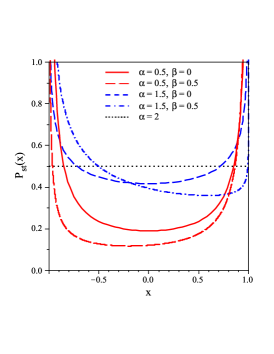
Figure 1: (Color online) Plots of the stationary probability density (15) for different values of the parameters $\alpha$ and $\beta$ and $l=1$.

References

- (1) J.-P. Bouchaud and A. Georges, Phys. Rep. 195, 127 (1990).
- (2) Lévy Flights and Related Topics in Physics, edited by M. F. Shlesinger, G. M. Zaslavsky, and U. Frisch (Springer-Verlag, Berlin, 1995).
- (3) A. V. Chechkin, V. Y. Gonchar, J. Klafter, and R. Metzler, Adv. Chem. Phys. 133, 439, (2006).
- (4) A. Ott, J.-P. Bouchaud, D. Langevin, and W. Urbach, Phys. Rev. Lett. 65, 2201 (1990).
- (5) T. H. Solomon, E. R. Weeks, and H. L. Swinney, Phys. Rev. Lett. 71, 3975 (1993).
- (6) H. Katori, S. Schlipf, and H. Walther, Phys. Rev. Lett. 79, 2221 (1997).
- (7) F. Bardou, J.-P. Bouchaud, A. Aspect, and C. Cohen-Tannoudji, Lévy Statistics and Laser Cooling (Cambridge University Press, Cambridge, 2002).
- (8) D. A. Benson, R. Schumer, R. M. W. Meerschaert, and S. W. Wheatcraft, Transp. Porous Media 42, 211 (2001).
- (9) B. Berkowitz, J. Klafter, R. Metzler, and H. Scher, Water Resour. Res. 38, 1191 (2002).
- (10) G. M. Viswanathan et al., Nature 381, 413 (1996).
- (11) D. Austin, W. D. Bowen, and J. I. McMillan, Oikos 105, 15 (2004).
- (12) B. Baeumer, M. Kovács, and M. Meerschaert, Bull. Math. Biol. 69, 2281 (2007).
- (13) A. M. Edwards et al., Nature 449, 1044 (2007).
- (14) B. V. Gnedenko and A. N. Kolmogorov, Limit Distributions for Sums of Independent Random Variables (Addison-Wesley, Cambridge, MA, 1954).
- (15) P. Langevin, C. R. Acad. Sci. 146, 530 (1908).
- (16) W. T. Coffey, Yu. P. Kalmykov, and J. T. Waldron, The Langevin Equation, 2nd ed. (World Scientific, Singapore, 2004).
- (17) P. D. Ditlevsen, Phys. Rev. E 60, 172 (1999).
- (18) S. Jespersen, R. Metzler, and H. C. Fogedby, Phys. Rev. E 59, 2736 (1999).
- (19) V. V. Yanovsky, A. V. Chechkin, D. Schertzer, and A. V. Tur, Physica A 282, 13 (2000).
- (20) D. Brockmann and I. M. Sokolov, Chem. Phys. 284, 409 (2002).
- (21) A. Dubkov and B. Spagnolo, Fluct. Noise Lett. 5, L267 (2005).
- (22) A. Janicki and A. Weron, Stat. Sci. 9, 109 (1994).
- (23) R. Weron, Stat. Probab. Lett. 28, 165 (1996).
- (24) B. Dybiec, E. Gudowska-Nowak, and P. Hänggi, Phys. Rev. E 75, 021109 (2007).
- (25) A. V. Chechkin, V. Yu. Gonchar, J. Klafter, R. Metzler, and L. V. Tanatarov, J. Stat. Phys. 115, 1505 (2004).
- (26) A. Dubkov and B. Spagnolo, Acta Phys. Pol. B 38, 1745 (2007).
- (27) W. Horsthemke and R. Lefever, Noise-Induced Transitions (Springer, Berlin, 1984).
- (28) P. Hänggi and P. Jung, Adv. Chem. Phys. 89, 239 (1995).
- (29) S. I. Denisov, A. N. Vitrenko, and W. Horsthemke, Phys. Rev. E 68, 046132 (2003).
- (30) N. G. Van Kampen, Stochastic Processes in Physics and Chemistry (North-Holland, Amsterdam, 1992).
- (31) P. Hänggi and H. Thomas, Phys. Rep. 88, 207 (1982).
- (32) P. Hänggi, Z. Phys. B 30, 85 (1978).
- (33) P. Hänggi, Z. Phys. B 36, 271 (1980).
- (34) N. G. van Kampen, Physica A 102, 489 (1980).
- (35) V. M. Zolotarev, One-Dimensional Stable Distributions (American Mathematical Society, Providence, 1986).
- (36) S. G. Samko, A. A. Kilbas, and O. I. Marichev, Fractional Integrals and Derivatives: Theory and Applications (Gordon and Breach, New York, 1993).
- (37) H. Risken, The Fokker-Planck Equation, 2nd ed. (Springer, Berlin, 1989).
- (38) H. Bateman and A. Erdélyi, Higher Transcendental Functions (McGraw-Hill, New York, 1953), Vol. 1.