Quantum improvement of time transfer between remote clocks
Abstract
Exchanging light pulses to perform accurate space-time positioning is a paradigmatic issue of physics. It is ultimately limited by the quantum nature of light, which introduces fluctuations in the optical measurements and leads to the so-called Standard Quantum Limit (SQL) Jaekel and Reynaud (1996a); Giovannetti et al. (2001, 2004). We propose a new scheme combining homodyne detection and mode-locked femtosecond lasers that lead to a new SQL in time transfer, potentially reaching the yoctosecond range (s). We prove that no other measurement strategy can lead to better sensitivity with shot noise limited light. We then demonstrate that this already very low SQL can be overcome using appropriately multimode squeezed light. Benefitting from the large number of photons used in the experiment and from the optimal choice of both the detection strategy and of the quantum resource, the proposed scheme represents a significant potential improvement in space-time positioning.
pacs:
42.50.Dv, 42.50.Lc, 42.62.EhAccurate spacetime positioning has become a crucial issue for future space experiments which require increasing resolution over large distances (see for example Bender et al. (2003)). The position in space (by ranging to a reference) or time (by clock synchronization with a reference) between two observers A and B may be achieved through the Einstein protocol which consists to repeatedly exchange light pulses Jaekel and Reynaud (1996b). From a fundamental point of view, this procedure is at the root of Einstein’s concept of space and time. From a more practical point of view, it permits to distribute the time standard over the whole earth and to precisely know the relative position of different satellites in space.
The basic principle relies on the property that, in the absence of dispersion, each pulse carries along its propagation a mean light cone variable which remains constant so that the measurement of the time of arrival of each pulse allows either a determination of distance or clock synchronization. The generic situation considered in this paper is the following (see figure (1)) : observer A regularly emits light pulses at a rate synchronized to its local clock; B receives these pulses and determine their times of arrival by measuring the difference between the arrival times of the incoming light pulses and light pulses delivered by a source located in B and synchronized to a reference clock in B. The accuracy of this measurement relies therefore on the precision of the clocks in A and B and on the sensitivity of the determination of the delay between two light pulses, that we will show how to optimize in the present paper.
Such a delay can be measured by at least two ways: the first one consists in measuring the arrival time of the maximum of the pulse envelope. We will refer to this procedure as a time-of-flight (tof) measurement. The second method consists in using the information contained in the phase of the electric field oscillation by making an interference pattern between the pulses arriving from A and a Local Oscillator (LO) derived from the local clock in B. This pattern will give the desired information if the phase of the pulse coming from A and the phase of the LO in B are locked to their respective local clocks. This method will be referred to as a phase (ph) measurement.
These measurement schemes suffer from quantum limits associated with the quantum nature of light Jaekel and Reynaud (1996a). For a coherent light pulse of central frequency and frequency spread , quantum fluctuations lead to the so called Standard Quantum Limit (SQL) of ranging for either time-of-flight Giovannetti et al. (2001) or phase Caves (1981); Jaekel and Reynaud (1990) measurements. Those expressions are given by
| (1) |
Where is the total number of photons measured in the experiment during the detection time. Let us briefly discuss those two SQL. First, it is clear on these expressions that the SQL can be as small as needed if one can use intense enough light, but there are obvious practical limitations to the energy carried by the light pulses. In contrast, isolated photons give rise to very low photon fluxes, and the corresponding SQL is very quickly a limitation of experimental protocols using photon counting techniques. The expressions also show that optical frequencies lead to much smaller SQL than microwave frequencies because of a larger and . Finally, as , the phase method has a better ultimate sensitivity than the time-of-flight technique but requires highly spatially and temporally coherent sources.
For the time being, the resolution in time transfer is limited by classical technical noises so that the previous SQL are not yet a limitation in time transfer. Nevertheless, with the recent developments in stabilization of frequency combs referenced to optical standard, it is getting closer and closer to these quantum limits Ma and al. (2004). Both for a fundamental point of view and for future experiments, it is therefore necessary to compute the ultimate sensitivity in time transfer with mode locked femtosecond laser since the latter combine both a time-of-flight information in their enveloppe, and a well stabilized phase information inside the enveloppe.
In order to compute the SQL in timing involving mode locked femtosecond lasers, we begin by writing the positive frequency electric field operator emitted by A in the absence of any perturbations, as a decomposition in temporal modes :
| (2) |
where is the measurement time. The orthonormal temporal modes will be written as a (complex) time-varying amplitude multiplied by a propagation phase factor of the form :
| (3) |
The annihilation operator corresponding to those modes are noted . Without any loss of generality, we can appropriately choose the mode basis such that the mean value of the electric field operator is proportional to , namely , with the mean number of photon and a global phase.
Now, any variation of the mean light cone variable, caused for example by a distance change between A and B, leads to a modification of the field received in B which reads (see figure (1)). The temporal mode corresponding to this field can be decomposed as follows if the perturbation is small :
| (4) |
The constant ensures the normalization of the new mode . The latter one will be called the timing mode because it carries the timing signal . For pulses of frequency spread 111We use the standard definition of the statistical frequency width : where is the Fourier transform of the enveloppe ., is given by and the expression of the timing mode is
| (5) |
is roughly equal to the number of field oscillations within the pulse, which can be as small as a few units for femtosecond pulses. The timing mode contains two terms: the first one, namely , gives a contribution to the timing signal via a phase change (interferometric method of ranging). The second one, namely , is normalized and orthogonal to so that it will be taken as the second mode of the basis . It reads :
| (6) |
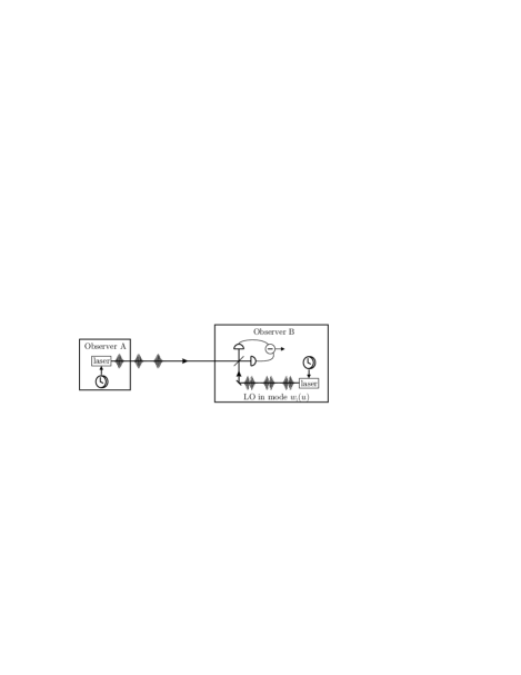
This mode gives a contribution to the timing signal via a time shift of the pulse enveloppe (time-of-flight technique). The latter mode is represented in the figure (2) and is the temporal analog of the spatial TEM01 gaussian mode when the emitted pulses are gaussian.
The timing signal can be retrieved by projecting on the timing mode . This can be done using the balanced homodyne detection scheme represented in figure (2) where the input pulses are mixed with a Local Oscillator (LO) put in the timing mode Delaubert et al. (2005), so that , with the mean number of photon in the LO field and its phase. Denoting the annihilation operators for the LO, the homodyne signal reads :
| (7) |
The mean signal of the balanced homodyne detection when a timing offset is present, then reads :
| (8) |
We assume from now on that, as usual, the LO is much more intense than the input field. The general case can be treated without difficulty. In this situation, the variance of the balanced homodyne signal, taken for , is given by :
| (9) |
where and are the variances of the quadrature operators (phase operator of mode ) and (amplitude operator of mode ) of the input field :
| (10) |
The Standard Quantum Limit (SQL) is then obtained as the smallest that can be measured using shot noise limited coherent light (), assuming a signal to noise ratio equal to one (). It is obtained for and is given by :
| (11) |
The expression (11) is one the main results of this paper and gives a new SQL in timing. The latter is lower than both the SQL in time-of-flight and phase measurements (see equation (1)), which obviously are special cases of our scheme when the LO is either in the or mode. This means that the proposed balanced homodyne detection scheme has a better sensitivity than existing schemes based on either time-of-flight or interferometric measurement. The improvement comes from the fact that coherent pulses, in addition to their phase, carries a time of flight information in their time varying enveloppe. Both informations are read by the balanced homodyne detection if the LO is shaped in the mode . Let us stress that such optimized measurements have already been successfully employed for pure phase measurement Berry and Wiseman (2004) and in the spatial domain to measure transverse beam displacement and tilt Treps et al. (2005).
For a mW laser with nm and a fs pulse duration, the SQL is equal to , i.e. a noise level of (20 yoctoseconds for one second integration time).
A natural question is to know whether it is possible to reach still better sensitivity on the same beam but by using another measurement strategy. An answer can be provided in the context of information theory with the help of the Cramer-Rao bound Réfrégier (2004), which gives the smallest measurable delay that can be achieved in the presence of a given distribution of noise. This bound has the property of being independent of the measurement strategy and depends only on the noise of the incoming signal. A calculation of the Cramer-Rao bound, analogous to the one detailed in Delaubert (2007); Delaubert et al. (2008) proves that using coherent light, this bound is precisely equal to the expression (11) of . We are therefore sure that no other measurement scheme will reach a better accuracy than the introduced balanced homodyne detection and in this sense this scheme is said to be efficient.
Obviously the SQL (11) is the fundamental limit when one restricts oneself to the use of classical states of light and coherent states, as proven with the previous standard Cramer-Rao bound. Nevertheless, it is well known that it can be beaten using quantum resources Giovannetti et al. (2004); Jozsa et al. (2000); Burgh and Bartlett (2005). For example, the improvement of the sensitivity in interferometric measurements using squeezed light has been proposed Caves (1981); Jaekel and Reynaud (1990), observed experimentally Xiao et al. (1987); Grangier et al. (1987); Barnett et al. (2003), and will be certainly practically implemented in the future generations of interferometric detectors of gravitational waves McKenzie et al. (2002). The use of an entangled photon source to improve time-of-flight ranging measurements in the photon-counting regime has been also proposed Giovannetti et al. (2001, 2002) and experimentally demonstrated Valencia et al. (2004) at a picosecond level of timing sensitivity. We propose here to improve the scheme introduced previously by using appropriately squeezed light.
Inspection of equation(9) immediately shows that in the case of a strong LO the signal to noise ratio is increased if the noise of the incoming mode is below the shot noise. This can be obtained if squeezing of the input field modes and is achieved along the quadratures and respectively. This therefore requires to first squeeze the phase of the input field and mix it with a squeezed vacuum mode Valcárcel et al. (2006), using procedures already demonstrated in the spatial domain Delaubert et al. (2005). If we assume that the squeezing coefficient is equal for the two states, namely ( being the squeezing parameter), then the new minimum measurable value of is given by :
| (12) |
This minimum resolvable is thus reduced below the SQL (11) by the factor . Note that the expression for the general case of different squeezing along and , as well as a LO not supposed strong, can be obtained straightforwardly from the equations given in the paper.
Using the best present technology, the noise reduction factor can reach dB Vahlbruch and al. (2007); Takeno et al. (2007), i.e. a factor of improvement, even at low noise frequencies. The advantage of squeezing over the other proposed quantum techniques such as entanglement is that it can be used together with an intense beam for which the SQL is already very low. In addition the squeezed beam travels along with the signal beam and therefore they both share commun noises. This is not the case for protocol using non local quantum correlations (such as most of the protocols based on entanglement) where the quantum correlations are spread over a large region of space and submitted to differential noise effects. The main drawback of squeezing is its sensitivity to losses in the optical system and the detectors. This means that the technique could be used in situations where light propagates in vacuum, for example between satellites in flying formation.
An experimental implementation of the scheme with the aim at reaching the SQL and then observe the quantum improvement suffers different technical challenges. First of all, reaching a timing precision in the yoctosecond regime requires very stable laser repetition rate and phase stabilization. This can be eventually be achieved with mode-locked femtosecond lasers which are already used for absolute and relative ranging in different measurement schemes Ye (2004); Minoshima and Matsumoto (2000); Towers and al. (2004); Joo and Kim (2004). The dominant source of noise in equation (9) is given by the noise of the phase of . Self-referencing stabilization using a beat allows to keep this noise to a very low level, down to rad/ at Hz with state-of-the-art stabilization techniques Fortier and al. (2002); Bartels et al. (2004), corresponding to a timing noise of s/ at Hz. Concerning the repetition rate , the latter can be locked to an optical reference, and current technology leads to a time jitter noise level of s/ at Hz Bartels et al. (2003); Shelton and al. (2002); Schibli and al. (2003). Another experimental challenge is to produce the squeezed temporal mode . Indeed, if the mode can be obtained with presently available commercial mode shapers Sato and al. (2002), the squeezing is much more challenging, but can in principle be obtained by propagation through a non-linear Kerr medium Schmitt et al. (1998) or more efficiently by using parametric down conversion pumped by mode-locked lasers Slusher et al. (1987); Rosenbluh and Shelby (1991), or even synchronously pumped OPOs Valcárcel et al. (2006).
Acknowledgements.
We are grateful to Serge Reynaud and Vincent Delaubert for fruitful discussions. Laboratoire Kastler Brossel is unité mixte de recherche (UMR) n of the CNRS.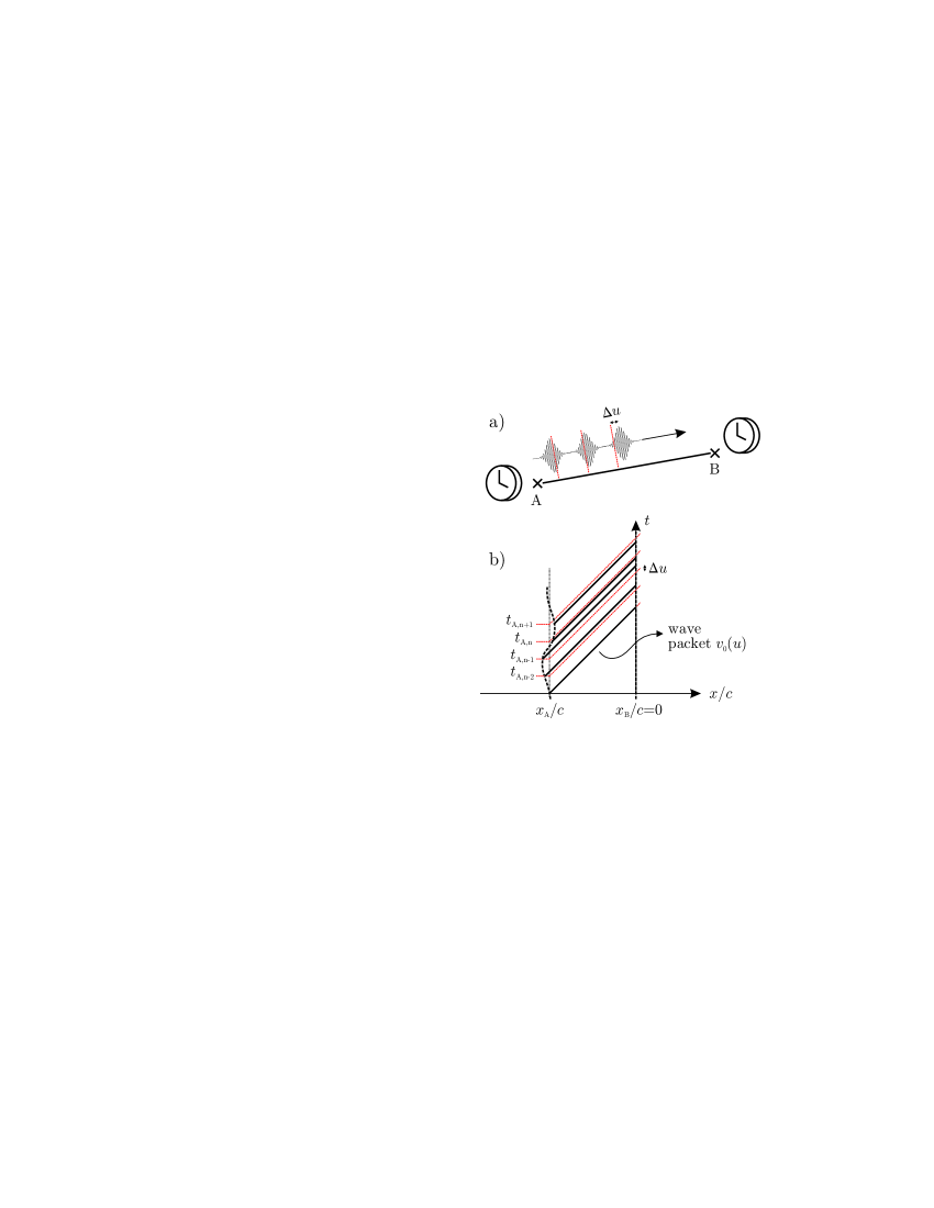
References
- Jaekel and Reynaud (1996a) M. Jaekel and S. Reynaud, Phys. Rev. Lett. 76, 2407 (1996a).
- Giovannetti et al. (2001) V. Giovannetti, S. Lloyd, and L. Maccone, Nature 412, 417 (2001).
- Giovannetti et al. (2004) V. Giovannetti, S. Lloyd, and L. Maccone, Science 306, 1330 (2004).
- Bender et al. (2003) P. Bender, J. Hall, J. Ye, and W. Klipstein, Space Science Reviews 108, 377 (2003).
- Jaekel and Reynaud (1996b) M.-T. Jaekel and S. Reynaud, Phys. Lett. A 220, 10 (1996b).
- Caves (1981) C. Caves, Phys. Rev. D 23, 1693 (1981).
- Jaekel and Reynaud (1990) M.-T. Jaekel and S. Reynaud, Europhys. Lett. 13, 301 (1990).
- Ma and al. (2004) L.-S. Ma and al., Science 303, 1843 (2004).
- Delaubert et al. (2005) V. Delaubert, N. Treps, C. Harb, P. Lam, and H.-A. Bachor, Optics Letters 31, 1537 (2005).
- Berry and Wiseman (2004) D. Berry and H. Wiseman, Phys. Rev. A 65, 043803 (2004).
- Treps et al. (2005) N. Treps, V. Delaubert, A. Ma tre, J. Courty, and C. Fabre, Phys. Rev. A 71, 013820 (2005).
- Réfrégier (2004) P. Réfrégier, Noise Theory and Application to Physics (Springer, 2004).
- Delaubert (2007) V. Delaubert, Ph.D. thesis, Université Pierre et Marie Curie (2007).
- Delaubert et al. (2008) V. Delaubert, N.Treps, C. Fabre, H. Bachor, and P. Réfrégier, EuroPhys. Lett. 81 (2008).
- Jozsa et al. (2000) R. Jozsa, D. Abrams, J. Dowling, and C. Williams, Phys. Rev. Lett. 85, 2010 (2000).
- Burgh and Bartlett (2005) M. D. Burgh and S. Bartlett, Phys. Rev. A 72, 042301 (2005).
- Xiao et al. (1987) M. Xiao, L.-A. Wu, and H. Kimble, Phys. Rev. Lett. 59, 278 (1987).
- Grangier et al. (1987) P. Grangier, R. Slusher, B. Yurke, and A. LaPorta, Phys. Rev. Lett. 59, 2153 (1987).
- Barnett et al. (2003) S. Barnett, C. Fabre, and A. Ma tre, Eur. Phys. J. D 22 (2003).
- McKenzie et al. (2002) K. McKenzie, D. Shaddock, D. McClelland, B. Buchler, and P. Lam, Phys. Rev. Lett. 88 (2002).
- Giovannetti et al. (2002) V. Giovannetti, S. Lloyd, and L. Maccone, Phys. Rev. A 65, 022309 (2002).
- Valencia et al. (2004) A. Valencia, G. Scarcelli, and Y. Shih, Appl. Phys. Letters 85, 2655 (2004).
- Valcárcel et al. (2006) G. D. Valcárcel, G. Patera, N. Treps, and C. Fabre, Phys. Rev. A 74, 061801(R) (2006).
- Vahlbruch and al. (2007) H. Vahlbruch and al., arXiv:0706.1431v1 [quant-ph] (2007).
- Takeno et al. (2007) Y. Takeno, M. Yukawa, H. Yonezawa, and A. Furusawa, Optics Express 15, 4321 (2007).
- Ye (2004) J. Ye, Optics Letters 29, 1153 (2004).
- Minoshima and Matsumoto (2000) K. Minoshima and H. Matsumoto, Applied Optics 39, 5512 (2000).
- Towers and al. (2004) C. Towers and al., Optics Letters 29, 2722 (2004).
- Joo and Kim (2004) K.-N. Joo and S.-W. Kim, Optics Express 14, 5954 (2004).
- Fortier and al. (2002) T. Fortier and al., Optics Letters 27, 1436 (2002).
- Bartels et al. (2004) A. Bartels, C. Oates, L. Hollberg, and S. Diddams, Optics Letters 29, 1081 (2004).
- Bartels et al. (2003) A. Bartels, S. Diddams, T. Ramond, and L. Hollberg, Optics Letters 28, 663 (2003).
- Shelton and al. (2002) R. Shelton and al., Optics Letters 27, 312 (2002).
- Schibli and al. (2003) T. Schibli and al., Optics Letters 28, 947 (2003).
- Sato and al. (2002) M. Sato and al., Jpn. J. Appl. Phys. 41, 3704 (2002).
- Schmitt et al. (1998) S. Schmitt, J. Ficker, M. Wolff, F. K nig, A. Sizmann, and G. Leuchs, Phys. Rev. Lett. 81 (1998).
- Slusher et al. (1987) R. Slusher, P. Grangier, A. LaPorta, B. Yurke, and M. J. Potasek, Phys. Rev. Lett. 59 (1987).
- Rosenbluh and Shelby (1991) M. Rosenbluh and R. Shelby, Phys. Rev. Lett. 66 (1991).