Abstract

In the multiple testing context, a challenging problem is the estimation of the proportion $\pi_{0}$ of true-null hypotheses. A large number of estimators of this quantity rely on identifiability assumptions that either appear to be violated on real data, or may be at least relaxed. Under independence, we propose an estimator $\widehat{\pi}_{0}$ based on density estimation using both histograms and cross-validation.
Due to the strong connection between the false discovery rate (FDR) and $\pi_{0}$, many multiple testing procedures (MTP) designed to control the FDR may be improved by introducing an estimator of $\pi_{0}$. We provide an example of such an improvement (plug-in MTP) based on the procedure of Benjamini and Hochberg. Asymptotic optimality results may be derived for both $\widehat{\pi}_{0}$ and the resulting plug-in procedure. The latter ensures the desired asymptotic control of the FDR, while it is more powerful than the BH-procedure.
Finally, we compare our estimator of $\pi_{0}$ with other widespread estimators in a wide range of simulations. We obtain better results than other tested methods in terms of mean square error (MSE) of the proposed estimator. Finally, both asymptotic optimality results and the interest in tightly estimating $\pi_{0}$ are confirmed (empirically) by results obtained with the plug-in MTP.

Keywords: multiple testing, false discovery rate, density estimation, histograms, cross-validation

Introduction

Multiple testing problems arise as soon as several hypotheses are tested simultaneously. Like in test theory, we are concerned with the control of type-I errors we may commit in falsely rejecting any tested hypothesis. Post-genomics, astrophysics or neuroimaging are typical areas in which multiple testing problems are encountered. For all these domains, the number of tests may be of the order of several thousands. Suppose we are testing each of $m$ hypotheses at level $0<\alpha<1,$ the probability of at least one false positive (e.g. false rejection) may equal $m\alpha$ in the worst case. A possible way to cope with this is to use the Bonferroni procedure (DPSB ), which consists in testing each hypothesis at level $\alpha/m.$ However, this method is known to be drastically conservative.
Since we may be more interested in controlling the proportion of false positives among rejections rather than the total number of false positives itself, Benjamini and Hochberg BH introduced the false discovery rate (FDR), defined by

$$FDR=\mathbb{E}\left[\frac{FP}{1\vee R}\right],$$

where $a\vee b=\max(a,b),$ $FP$ denotes the number of false positives and $R$ is the total number of rejections. A large part of the literature is devoted to the building of multiple testing procedures (MTP) that upper bound FDR as tightly as possible (BKY ; BY ). For instance, that of Benjamini and Hochberg (BH-procedure) BH ensures the following inequality under independence

$$FDR\leq\pi_{0}\alpha\leq\alpha,$$

where $\pi_{0}$ denotes the unknown proportion of true null hypotheses, while $\alpha$ is the actual level at which we want to control the FDR. Since $\pi_{0}$ is unknown, the BH-procedure suffers some loss in power, which is all the more deep as $\pi_{0}$ is small. A natural idea to overcome this drawback is the computation of an accurate $\pi_{0}$ estimator, which would be plugged in the procedure. Thus $\pi_{0}$ appears as a crucial quantity that is to be estimated, hence the large amount of existing estimators. We refer to LLF ; Bro for reviews on this topic. The randomness of this estimation needs to be taken into account in the assessment of the procedure performance (GW04 ; Sto02 ).
In many of quite recent papers about multiple testing (see Bro ; Efr04 ; ETST ; GW04 ), a two-component mixture density is used to describe the behaviour of p-values associated with the $m$ tested hypotheses. As usual for mixture models, we need an assumption that ensures the identifiability of the model parameters. Thus, most of $\pi_{0}$ estimators rely on the strong assumption that there are only p-values following a uniform distribution on $[0,1]$ in a neighbourhood of 1. However, Pounds et al. PC recently observed the violation of this key assumption. They pointed out that some p-values associated with induced genes may be artificially sent near to 1, for example when a one-sided test is performed while the non-tested alternative is true. To overcome this difficulty, we propose to estimate the density of p-values by some non-regular histograms, providing a new estimator of $\pi_{0}$ that remains reliable in the Pounds’ framework thanks to a relaxed ”identifiability assumption”.
In the context of density estimation with the quadratic loss and histograms, asymptotic considerations have been used by Scott (Sco79 ) for instance. A drawback of this approach relies on regularity assumptions made on the unknown distribution. Some AIC-type penalized criteria as in Barron et al. BBM could be applied as well. However, such an approach depends on some unknown constants that have to be calibrated at the price of an intensive simulation step (see Leb in the regression framework). As it is both regularity-assumption free and computationally cheap, we address the problem by means of cross-validation, first introduced in this context by Rudemo (Rud ). More precisely, the leave-p-out cross-validation (LPO) is successfully applied following a strategy exposed in Celisse et al. CR07 . Unlike Schweder and Spjøtvoll’s estimator of $\pi_{0}$ (SS82 ), ours is fully adaptive thanks to the LPO-based approach, e.g. it does not depend on any user-specified parameter.
The paper is organized as follows. In Section 1, we present a cross-validation based estimator of $\pi_{0}$ (denoted by $\widehat{\pi}_{0}$). Our main assumptions are specified and a description of the whole $\pi_{0}$ estimation procedure is given. Section 2 is devoted to asymptotic results such as consistency of $\widehat{\pi}_{0}$. Then we propose a plug-in multiple testing procedure (plug-in MTP), based on the same idea as that of Genovese et al. GW04 . It is compared to the BH-procedure in terms of power and its asymptotic control of the FDR is derived. Section 3 is devoted to the assessment of our $\pi_{0}$ estimation procedure in a wide range of simulations. A comparison with other existing and widespread methods is carried out.The influence of the $\pi_{0}$ estimation on the power of the plug-in MTP is inferred as well. This study results in almost overall improved estimations of the proposed method.

1 Estimation of the proportion of true null hypotheses

1.1 Mixture model

Let $P_{1},\dots,P_{m}$ be $m$ i.i.d. random variables following a density $g$ on $[0,1].$ $P_{1},\ldots,P_{m}$ denote the p-values associated with the $m$ tested hypotheses. Taking into account the two populations of (${\bf H}_{0}$ and ${\bf H}_{1}$) hypotheses, we assume (Bro ; Efr04 ; GW04 ) that $g$ may be written as

$$\forall x\in[0,1],\qquad g(x)=\pi_{0}f_{0}(x)+(1-\pi_{0})f_{1}(x),$$

where $f_{0}$ (resp. $f_{1}$) denotes the density of ${\bf H}_{0}$ (resp. ${\bf H}_{1}$) p-values, that is p-values corresponding to true null (resp. false null) hypotheses. $\pi_{0}$ is the unknown proportion of true null hypotheses. Moreover, we assume that $f_{0}$ is continuous, which ensures that $f_{0}=1$: ${\bf H}_{0}$ p-values follow the uniforme distribution $\mathcal{U}([0,1]).$ Subsequently, the above mixture becomes

$$\forall x\in[0,1],\qquad g(x)=\pi_{0}+(1-\pi_{0})f_{1}(x),$$ (1)

where both $\pi_{0}$ and $f_{1}$ remain to be estimated.
Most of existing $\pi_{0}$ estimators rely on a sufficient condition which ensures the identifiability of $\pi_{0}.$ This assumption may be expressed as follows

$$\exists\lambda^{*}\in]0,1]/\quad\forall i\in\{1,\ldots,m\},\ P_{i}\in[\lambda^{*},1]\Rightarrow P_{i}\sim\mathcal{U}([\lambda^{*},1]).\qquad(\mathbf{A})$$

(A) is therefore at the origin of Schweder and Spjøtvoll’s estimator (SS82 ), further studied by Storey (Sto02 ; STS ). It depends on a cut-off $\lambda\in[0,1]$ from which only ${\bf H}_{0}$ p-values are observed. This estimation procedure is further detailed in Section 3. The same idea underlies the adaptive Benjamini and Hochberg step-up procedure described in BKY , based on the slope of the cumulative distribution function of p-values. If we assume $\lambda^{*}=1$ (that is $f_{1}(1)=0$), Grenander Gre and Storey et al. ST choose $\widehat{g}(1)$ to estimate $\pi_{0}$, where $\widehat{g}$ denotes the estimator of $g$. Genovese et al. GW04 use $(1-G(t))/(1-t),\ t\in(0,1)$ as an upper bound of $\pi_{0}$, which becomes (for $t$ large enough) an estimator as soon as (${\bf A}$) is true.
However, this assumption may be strongly violated as noticed by Pounds et al. PC . This point is detailed in Section 3.2. Following this remark, we propose the milder assumption (${\bf A}^{\prime}$):

$$\exists\Lambda^{*}=[\lambda^{*},\mu^{*}]\subset(0,1]/\quad\forall i\in\{1,\ldots,m\},\ P_{i}\in\Lambda^{*}\Rightarrow P_{i}\sim\mathcal{U}(\Lambda^{*}).\qquad({\bf A}^{\prime})$$

While it is a generalization of (${\bf A}$), this assumption remains true in Pounds’ framework as we will see in Section 3.2 . Scheid et al. SS04 proposed a procedure named $Twilight$, which consists in a penalized criterion and provides, as a by-product, an estimation of $\pi_{0}$. Since this procedure does not rely on assumption (A), it should be taken as a reference competitor in the simulation study (Section 3) with respect to our proposed estimators.

1.2 A leave-$p$-out based density estimator

If $g$ satisfies $(\textbf{A'})$, any ”good estimator” of this density on $\Lambda^{*}$ would provide an estimate of $\pi_{0}.$ Since $g$ is constant on the whole interval $\Lambda^{*},$ we adopt histogram estimators. Note that we do not really care about the rather poor approximation properties of histograms outside of $\Lambda^{*}$ as our goal is essentially the estimation of $\Lambda^{*}$ and of the restriction of $g$ to $\Lambda^{*}$, denoted by $g_{|\Lambda^{*}}$ in the sequel.
For a given sample of observations $P_{1},\dots,P_{m}$ and a partition of $[0,1]$ in $D\in\mathbb{N}^{*}$ intervals $I=(I_{k})_{k=1,\dots,D}$ of respective length $\omega_{k}=|I_{k}|,$ the histogram $\widehat{s}_{\omega}$ is defined by

$$\forall x\in[0,1],\qquad\widehat{s}_{\omega}(x)=\sum_{k=1}^{D}\frac{m_{k}}{m\,\omega_{k}}\hbox{ 1\hskip-2.7pt{I}}_{I_{k}}(x),$$

where $m_{k}=\sharp\{i\in\hbox{ $\mathrm{[}$\hskip-4.2pt{$\mathrm{[}\,$}}1,m\hbox{$\,\mathrm{]}$\hskip-4.2pt{$\mathrm{]}\,$}}:\,P_{i}\in I_{k}\}.$
If we denote by $\mathcal{S}$ the collection of histograms we consider, the ”best estimator” among $\mathcal{S}$ is defined in terms of the quadratic risk:

$$\widetilde{s} = \mathop{\mathrm{Argmin}}_{s\in\mathcal{S}}\mathbb{E}_{g}\left[||g-s||_{2}^{2}\right],$$ (2)

$$= \mathop{\mathrm{Argmin}}_{s\in\mathcal{S}}\left\{\mathbb{E}_{g}\left[||s||_{2}^{2}\right]-2\int_{[0,1]}s(x)g(x)\,dx\right\},$$

where the expectation is taken with respect to the unknown $g$. According to (2), we define $R$ by

$$R(s)=\mathbb{E}_{g}\left[||s||_{2}^{2}\right]-2\int_{[0,1]}s(x)g(x)\,dx.$$ (3)

In (3) we notice that $R$ still depends on $g$ that is unknown. To get rid of this, we use a cross-validation estimator of $R$ that will achieve the best trade-off between bias and variance. Following (HTF ), we know that leave-one-out (LOO) estimators may suffer from some high level variability. For this reason we prefer the use of leave-$p$-out (LPO), keeping in mind that the choice of the parameter $p$ will enable the control of the bias-variance trade-off.
At this stage, we refer to Celisse et al. CR07 for an exhaustive presentation the leave-p-out (LPO) based strategy. Hereafter, we remind the reader what LPO cross-validation consists in and then, give the main steps of the reasoning. First of all, it is based on the same idea as the well-known leave-one-out (see HTF for an introduction) to which it reduces for $p=1.$ For a given $p\in\hbox{ $\mathrm{[}$\hskip-4.2pt{$\mathrm{[}\,$}}1,m-1\hbox{$\,\mathrm{]}$\hskip-4.2pt{$\mathrm{]}\,$}}$, let split the sample $P_{1},\dots,P_{m}$ into two subsets of respective size $m-p$ and $p$. The first one, called training set, is devoted to the computation of the histogram estimator whereas the second one (the test set) is used to assess the behaviour of the preceding estimator. These two steps have to be repeated $m\choose p$ times, which is the number of different subsets of cardinality $p$ among $\{P_{1},\dots,P_{m}\}.$

Closed formula of the LPO risk

This outlined description of the LPO leads to the following closed formula for the LPO risk estimator of $R(\widehat{s}_{\omega})$ (see CR07 ): For any partition $I=(I_{k})_{k=1,\dots,D}$ of $[0,1]$ in $D$ intervals of length $\omega_{k}=|I_{k}|$ and $p\in\hbox{ $\mathrm{[}$\hskip-4.2pt{$\mathrm{[}\,$}}1,m-1\hbox{$\,\mathrm{]}$\hskip-4.2pt{$\mathrm{]}\,$}},$

$$\widehat{R}_{p}(\omega)=\frac{2m-p}{(m-1)(m-p)}\sum_{k=1}^{D}\frac{m_{k}}{m\omega_{k}}-\frac{m(m-p+1)}{(m-1)(m-p)}\sum_{k=1}^{D}\frac{1}{\omega_{k}}\left(\frac{m_{k}}{m}\right)^{2},$$ (4)

where $m_{k}=\sharp\{i\in\hbox{ $\mathrm{[}$\hskip-4.2pt{$\mathrm{[}\,$}}1,m\hbox{$\,\mathrm{]}$\hskip-4.2pt{$\mathrm{]}\,$}}:\ P_{i}\in I_{k}\},$ $k=1,\dots,D.$ As it may be evaluated with a computational complexity of only $O\left(m\log m\right)$, (4) means that we have a very efficient estimator of the quadratic risk $R(\widehat{s}_{\omega})$. Now, we propose a strategy for the choice of $p$ that relies on the minimization of the mean square error criterion (MSE) of our LPO estimator of the risk. Indeed among $\{\widehat{R}_{p}(\widehat{s}_{\omega}):\ p\in\hbox{ $\mathrm{[}$\hskip-4.2pt{$\mathrm{[}\,$}}1,m-1\hbox{$\,\mathrm{]}$\hskip-4.2pt{$\mathrm{]}\,$}}\},$ we would like to choose the estimator that achieves the best bias-variance trade-off. This goal is reached by means of the MSE criterion, defined as the sum of the square bias and the variance of the LPO risk estimator. Thanks to (4), closed formulas for both the bias (5) and the variance (6) of LPO risk estimator may be derived. We recall here these expressions that come from CR07 .

Bias and variance of the LPO risk estimator

Let $\omega$ correspond to a $D-$partition $(I_{k})_{k}$ of $[0,1]$ and for any $k\in\{1,\dots,D\},$ $\alpha_{k}=\Pr[P_{1}\in I_{k}]$ such that $\alpha=(\alpha_{1},\dots,\alpha_{D})\in[0,1]^{D}.$
Then for any $p\in\hbox{ $\mathrm{[}$\hskip-4.2pt{$\mathrm{[}\,$}}1,m-1\hbox{$\,\mathrm{]}$\hskip-4.2pt{$\mathrm{]}\,$}}$,

$$B_{p}(\omega) = B_{p}(\alpha,\omega)=\frac{p}{m(m-p)}\sum_{k=1}^{D}\frac{\alpha_{k}(1-\alpha_{k})}{\omega_{k}}\,,$$ (5)

$$V_{p}(\omega) = V_{p}(\alpha,\omega)=\frac{p^{2}\varphi_{2}(m,\alpha,\omega)+p\,\varphi_{1}(m,\alpha,\omega)+\varphi_{0}(m,\alpha,\omega)}{[m(m-1)(m-p)]^{2}}\,,$$ (6)

where

$$\forall(i,j) \in \{1,\dots,3\}\times\{1,2\},\quad s_{i,j}=\sum_{k=1}^{D}\alpha_{k}^{i}/\omega_{k}^{j},$$

$$\varphi_{2}(m,\alpha,\omega) = 2m(m-1)\left[(m-2)(s_{2,1}+s_{1,1}-s_{3,2})-ms_{2,2}-(2m-3)s_{2,1}^{2}\right]\,,$$

$$\varphi_{1}(m,\alpha,\omega) = -2m(m-1)(3m+1)\left[(m-2)(s_{2,1}-s_{3,2})-ms_{2,2}\right]+$$

$$2m(m-1)\left[2(m+1)(2m-3)s_{2,1}^{2}+(-3m^{2}+3m+4)s_{1,1}\right]\,,$$

$$\varphi_{0}(m,\alpha,\omega) = 4m(m-1)(m+1)\left[(m-2)(s_{2,1}-s_{3,2})-ms_{2,2}\right]-$$

$$2m(m-1)\left[(m^{2}+2m+1)(2m-3)s_{2,1}^{2}+(2m^{3}-4m-2)s_{1,1}\right]+$$

$$m(m-1)^{2}(s_{1,2}-s_{1,1}^{2})\,.$$

Plug-in estimators may be obtained from the preceding quantities by just replacing $\alpha_{k}$ with $\widehat{\alpha}_{k}=m_{k}/m$ in the expressions. Following our idea about the choice of $p$, we define for each (partition) $\omega$ the best theoretical value $p^{*}$ as the minimum location of the MSE criterion:

$$p^{*}=\mathop{\mathrm{Argmin}}_{p\in\hbox{ $\mathrm{[}$\hskip-4.2pt{$\mathrm{[}\,$}}1,m-1\hbox{$\,\mathrm{]}$\hskip-4.2pt{$\mathrm{]}\,$}}}MSE(p)=\mathop{\mathrm{Argmin}}_{p}\left\{B_{p}(\omega)^{2}+V_{p}(\omega)\right\}.$$ (7)

The main point is that this minimization problem has an explicit solution named $p_{\mathbb{R}}^{*}$, as stated by Theorem 3.1 in CR07 . For the sake of clarity, we recall the MSE expression:

Minimum location expression

With the same notations as for the bias and the variance, we obtain for any $x\in\mathbb{R}$,

$$MSE(x)=\frac{x^{2}[\varphi_{3}(m,\alpha,\omega)+\varphi_{2}(m,\alpha,\omega)]+x\,\varphi_{1}(m,\alpha,\omega)+\varphi_{0}(m,\alpha,\omega)}{\left[m(m-1)(m-x)\right]^{2}}\,,$$

where $\varphi_{3}(m,\alpha,\omega)=(m-1)^{2}(s_{1,1}-s_{2,1})^{2}.$
Thus, we define our best choice $\widehat{p}$ for the parameter $p$ by

$$\widehat{p}=\left|\begin{array}[]{ll}k\left(\widehat{p}_{\mathbb{R}}\right)\,,&\mathrm{if}\ \widehat{p}_{\mathbb{R}}\in[1,m-1]\\ 1,&\mathrm{otherwise}\end{array}\right.,$$ (8)

where $k(x)$ denotes the closest integer near to $x$ and $\widehat{p}_{\mathbb{R}}$ has the same definition as $p^{*}_{\mathbb{R}}$, but with $\widehat{\alpha}$ instead of $\alpha$ in the expression.
Remark: There may be a real interest in choosing adaptively the parameter $p$, rather than fixing $p=1$. Indeed in the regression framework for instance, Shao Shao93 and Yang Yang07 underline that the simple and widespread LOO may be sub-optimal with respect to LPO with a larger $p$. In the linear regression set-up, Shao even shows that $p/m\to 1$ as $m\to+\infty$ is necessary to get consistency in selection.

1.3 Estimation procedure of $\pi_{0}$

1.3.1 Collection of non-regular histograms

We now precise the specific collection of histograms we will consider. For given integers $N_{min}<N_{max},$ we build a regular grid of $[0,1]$ in $N$ intervals (of length $1/N$) with $N\in\hbox{ $\mathrm{[}$\hskip-4.2pt{$\mathrm{[}\,$}}N_{min},N_{max}\hbox{$\,\mathrm{]}$\hskip-4.2pt{$\mathrm{]}\,$}}.$ For a couple of integers $0\leq k<\ell\leq N$, we define a unique histogram made of first $k$ regular columns of width $1/N$, then a wide central column of length $(\ell-k)/N$ and finally $N-\ell$ thin regular columns of width $1/N.$ An example of such an histogram is given in Figure 1.

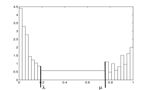
Figure 1: Example of non-regular histogram in $\mathcal{S}$. There are $k=7$ regular columns from $0$ to $\lambda=k/N$, a wide central column from $\lambda$ to $\mu=\ell/N$, and $N-\ell=7$ regular column of width $1/N$ from $\mu$ to 1.

The collection $\mathcal{S}$ of the histograms we consider is defined by

$$\mathcal{S}=\bigcup_{N\in\hbox{ $\mathrm{[}$\hskip-4.2pt{$\mathrm{[}\,$}}N_{min},N_{max}\hbox{$\,\mathrm{]}$\hskip-4.2pt{$\mathrm{]}\,$}}}\mathcal{S}_{N},$$

where

$$\forall N,\qquad\mathcal{S}_{N}=\left\{\widehat{s}_{\omega}\ :\ w_{k+1}=(\ell-k)/N,\ w_{i}=1/N\ for\ i\neq k+1,\ 0\leq k<\ell\leq N\right\}.$$

Provided $(\mathbf{A^{\prime}})$ is fulfilled, we expect for each $N$ a selected histogram with its wide central interval $[\lambda,\mu]$ close to $\Lambda^{*}$. The comparison of all these histograms (one per value of $N$) enables to relax the dependence of each selected histogram on the grid width $1/N.$

1.3.2 Estimation procedure

Following the idea at the beginning of Section 1.2, $\widehat{\pi}_{0}$ will consist of the height of the selected histogram on its central interval $[\lambda,\mu]$. More precisely, we propose the following estimation procedure for $\pi_{0}.$ For each partition (represented here by the vector $\omega$), we compute $\widehat{p}\,(\omega)=\mathop{\mathrm{Argmin}}_{p}\widehat{MSE}(p,\omega),$ where $\widehat{MSE}$ denotes the MSE estimator obtained by plugging $m_{k}/m$ in place of $\alpha_{k}$ in expressions of (7). The best (in terms of the bias-variance trade-off) LPO estimator of the quadratic risk $R(\widehat{s}_{\omega})$ is therefore $\widehat{R}_{\widehat{p}(\omega)}(\omega)$. Then we choose the histogram that reaches the minimum of the latter criterion over $\mathcal{S}.$ From this histogram, we finally get both the interval $[\widehat{\lambda},\widehat{\mu}]$, which estimates $\Lambda^{*}$, and

$$\widehat{\pi}_{0}=\widehat{\pi}_{0}(\widehat{\lambda},\widehat{\mu})\stackrel{{\scriptstyle def}}{{=}}\frac{\sharp\left\{i:\,P_{i}\in\left[\widehat{\lambda},\widehat{\mu}\right]\right\}}{m(\widehat{\mu}-\widehat{\lambda}\,)}\,\cdot$$

These steps are outlined hereafter
Procedure:

1. For each partition denoted by $\omega$, define $\widehat{p}\,(\omega)=\mathop{\mathrm{Argmin}}_{p}\widehat{MSE}(p,\omega).$

2. Find the best partition $\widehat{\omega}=\mathop{\mathrm{Argmin}}_{\omega}\widehat{R}_{\widehat{p}(\omega)}(\omega).$

3. From $\widehat{\omega}$, get $(\widehat{\lambda},\widehat{\mu}).$

4. Compute the estimator  $\widehat{\pi}_{0}=\frac{\sharp\left\{i:\,P_{i}\in\left[\widehat{\lambda},\widehat{\mu}\right]\right\}}{m(\widehat{\mu}-\widehat{\lambda}\,)}\,\cdot$

2 Asymptotic results

2.1 Pointwise convergence of LPO risk estimator

Lemma 2.1.

Following the notations in Section 1.2, for any $p\in\{1,m-1\}$ and $\omega$, we have

$$MSE(p,\omega)=\mathcal{O}_{m\to+\infty}\left(1/m\right),$$

Moreover if $s_{2,2}+s_{3,2}-s_{1,1}-s_{2,1}\neq 0,$

$$\widehat{p}(\omega)/m\xrightarrow[m\to+\infty]{a.s.}\ell_{\infty}(\omega),$$

where $\ell_{\infty}(\omega)\in[0,1].$

Proof.

2. We see that

   $$\varphi_{3}+\varphi_{2} = 2m^{3}[s_{2,1}+s_{1,1}-s_{3,2}-s_{2,2}-2s_{2,1}^{2}]+o(m^{3}),$$

   $$\varphi_{1} = 2m^{4}[3s_{3,2}+3s_{2,2}-3s_{2,1}+4s_{2,1}^{2}-3s_{1,1}]+o(m^{4}),$$

   $$\varphi_{0} = -4m^{5}[s_{2,1}^{2}+s_{1,1}]+o(m^{5}).$$

   Thus for any $p\in\{1,\dots,m-1\}$ and partition of size vector $\omega\in[0,1]^{D}$ we have

   $$MSE(p,\omega)=\mathcal{O}_{m\to+\infty}\left(\frac{1}{m}\right)\,\cdot$$

3. Simple calculations lead to

   $$\frac{p_{\mathbb{R}}^{*}(\omega)}{m}\xrightarrow[m\to+\infty]{}\frac{3(s_{2,1}-s_{3,2}-s_{2,2})+7s_{1,1}}{s_{1,1}+s_{2,1}-s_{2,2}-s_{3,2}}=\ell(\alpha,\omega).$$

   As for any $k$ $\widehat{\alpha}_{k}\xrightarrow[m\to+\infty]{a.s.}\alpha_{k},$ the continuous mapping theorem implies the almost surely convergence. Finally, the result follows by setting $\widehat{\ell}(\omega)=\ell(\widehat{\alpha},\omega)$ and $\ell_{\infty}(\omega)=\hbox{ 1\hskip-2.7pt{I}}_{\{\ell(\alpha,\omega)\in[0,1]\}}\ell(\alpha,\omega).$

∎

Proposition 2.1.

For any given $\omega,$ define $\widehat{p}(\omega)$ as in Section 1.2 and $\widehat{L}_{p}(\omega)=\widehat{R}_{p}(\omega)+||g||_{2}^{2}.$ If $\ell_{\infty}(\omega)\neq 1,$ we have

$$\widehat{L}(\omega)\stackrel{{\scriptstyle def}}{{=}}\widehat{L}_{\widehat{p}}(\omega)\xrightarrow[m\to+\infty]{P}L(\omega)\stackrel{{\scriptstyle def}}{{=}}||g-s_{\omega}||_{2}^{2}.$$

Remark: Note that the assumption on $\ell_{\infty}$ does seem rather natural. It means that the test set must be (at most) of the same size as the training set ($\widehat{p}/(n-\widehat{p})=\mathcal{O}_{P}(1)$). Moreover, $\ell_{\infty}(\omega)=1$ if and only if $s_{2,1}-s_{2,2}-s_{3,2}=-3\,s_{1,1},$ that holds for very specific densities.

Proof.

The first part of Lemma 2.1 implies that $\widehat{R}_{p}(\omega)-R(\widehat{s}_{\omega})\xrightarrow[m\to+\infty]{P}0.$ Combined with $R(\widehat{s}_{\omega})\xrightarrow[m\to\infty]{}L(\omega)-||g||_{2}^{2},$ it yields that for any fixed $p$,

$$\widehat{L}_{p}(\omega)\xrightarrow[m\to+\infty]{P}L(\omega).$$

Finally, the result follows from both the continuous mapping theorem and the assumption on $\ell_{\infty}.$ ∎

2.2 Consistency of $\widehat{\pi}_{0}$

We first emphasize that for a given $N\in\{N_{\min},\dots,N_{\max}\}$ any histogram in $\mathcal{S}_{N}$ is associated with a given partition of $[0,1]$ that may be uniquely represented by $(N,\lambda,\mu)$. We give now the first lemma of the consistency proof.

Lemma 2.2.

For $\lambda^{*}\neq\mu^{*}\in[0,1],$ let $s$ be a constant density on $[\lambda^{*},\mu^{*}]$. Suppose $N_{\min}$ such that for any $N_{\min}\leq N,$ it exists a partition $(N,\lambda,\mu)$ satisfying $0<\mu-\lambda\leq\mu^{*}-\lambda^{*}.$ For a given $N,$ let $\omega_{N}$ represent the partition $(N,\lambda_{N},\mu_{N})$ with $\lambda_{N}=\lceil N\lambda^{*}\rceil/N$ and $\mu_{N}=\lfloor N\mu^{*}\rfloor/N.$ Define $s_{\omega}$ as the orthogonal projection of $s$ onto piecewise constant functions built from the partition associated with $\omega.$ If the dimension of a partition is its number of pieces, then $\omega_{N}$ is the partition with the smallest dimension satisfying

$$\omega_{N}\in\mathop{\mathrm{Argmin}}_{\omega}||s-s_{\omega}||_{2}^{2}.$$

Proof.

For symmetry reasons, we deal with partitions, for a given $N,$ made of regular columns of width $1/N$ from 0 to $\lambda$ and only one column from $\lambda$ to 1 (e.g. we set $\mu=1$). In the sequel, $I^{(N)}$ denotes the partition associated with $\omega_{N}$.

1. Suppose that it exists $\omega_{0}$ such that $s=s_{\omega_{0}}.$ Then $||s-s_{\omega_{N}}||_{2}^{2}=0$ and $\omega_{N}\in\mathop{\mathrm{Argmin}}_{\omega}||s-s_{\omega}||_{2}^{2}$.

2. Otherwise, $s$ does not equal to any $s_{\omega}$.

   1. If $\lambda^{*}=k/N,$ then $\lambda_{N}=\lambda^{*}.$ Any subdivision $I$ of $I^{(N)}$ satisfies $||s-s_{\omega}||_{2}^{2}=||s-s_{\omega_{N}}||_{2}^{2},$ where $\omega$ corresponds to $I$. Now, let $\mathcal{F}_{I}$ be the set of piecewise constant functions built from a partition $I$. For any partition $I=(I_{k})_{k}$ such that $\forall k,\ I^{(N)}_{\ell}\subset I_{k}$ for a given $\ell,$ then $\mathcal{F}_{I}\subset\mathcal{F}_{I^{(N)}}.$ Thus $||s-s_{\omega}||_{2}^{2}=||s-s_{\omega_{N}}||_{2}^{2}+||s_{\omega_{N}}-s_{\omega}||_{2}^{2},$ since $s_{\omega_{N}}-s_{\omega}\in\mathcal{F}_{I^{(N)}}.$ Therefore, $\omega_{N}\in\mathop{\mathrm{Argmin}}_{\omega}||s-s_{\omega}||_{2}^{2}.$

   2. If $\lambda^{*}\not\in\{1/N,\dots,1\}$. As before, any subdivision of $I^{(N)}$ will have the same bias, whereas it is larger for any partition containing $I^{(N)}$. So, $\omega_{N}\in\mathop{\mathrm{Argmin}}_{\omega}||s-s_{\omega}||_{2}^{2}.$

∎

Lemma 2.3.

With the same notations as before, we define $L(\omega)=||s-s_{\omega}||_{2}^{2}$. Let $\widehat{L}$ be a random process indexed by the set of partitions $\Omega$ such that $\widehat{L}(\omega^{\prime})\xrightarrow[m\to+\infty]{P}L(\omega^{\prime}),$ for any $\omega^{\prime}\in\Omega$. If $\widehat{\omega}\in\mathop{\mathrm{Argmin}}_{\omega}\widehat{L}(\omega),$ then

$$\widehat{L}(\widehat{\omega})\xrightarrow[m\to+\infty]{P}\min\{L(\omega):\,\omega\in\Omega\}.$$

Proof.

Set $\Gamma\subset\Omega$ such that $\forall\omega\in\Gamma,\ L(\omega)=\min_{\omega^{\prime}\in\Omega}L(\omega^{\prime})$ and define $\delta=\min_{\omega\neq\omega^{\prime}\in\Gamma}|L(\omega)-L(\omega^{\prime})|/2$. For $|\Omega|=k$ and $|\Gamma|=\ell,$ we have the ordered quantities $L(\omega^{1})=\dots=L(\omega^{k})<L(\omega^{k+1})\leq\dots\leq L(\omega^{\ell})$. Set $\epsilon>0$. For each $\omega^{i},$ it exists $m_{i}$ (large enough) such that for $m\geq m_{i},\ |\widehat{L}(\omega^{i})-L(\omega^{i})|<\epsilon$, with high probability. For $m_{\max}=\max_{i}m_{i}$, we get $\max_{\omega\in\Omega}|\widehat{L}(\omega)-L(\omega)|<\epsilon$ in probability. Thanks to the latter inequality and by definition of $\widehat{\omega}$,

$$L(\widehat{\omega})<\widehat{L}(\widehat{\omega})+\epsilon\leq\widehat{L}(\omega)+\epsilon<L(\omega)+2\epsilon,\ \mathrm{in\ Probability}$$

for any $\omega\in\Omega\setminus\Gamma.$ Hence, we obtain

$$L(\widehat{\omega})<\min_{\omega\in\Omega\setminus\Gamma}L(\omega)=L(\omega^{k+1}),\ \mathrm{in\ Probability}.$$

Thus, $\widehat{\omega}\in\Gamma$ with high probability and the result follows. ∎

Theorem 2.1.

For $0\leq\lambda^{*}<\mu^{*}\leq 1,$ let $s:\;[0,1]\mapsto[0,1]$ be a constant function on $[\lambda^{*},\mu^{*}]$ such that $s$ is not constant on any interval $I$ with $[\lambda^{*},\mu^{*}]\varsubsetneq I$ (if it exists). Suppose $N_{\min}$ such that for any $N_{\min}\leq N\leq N_{\max},$ it exists a partition $(N,\lambda,\mu)$ satisfying $0<\mu-\lambda\leq\mu^{*}-\lambda^{*}.$ Set $\Omega=\cup_{N}\Omega_{N}$, where $\Omega_{N}$ denotes the partitions associated with $S_{N}$. If $\widehat{\pi}_{0}$ is the estimator described in Section 1.3.2 selected from $\Omega$, then

$$\widehat{\pi}_{0}\xrightarrow[m\to+\infty]{P}\pi_{0}.$$

Proof.

For $\epsilon>0$ and $N_{\min}\leq N\leq N_{\max}$,

$$\Pr\left[\,|\pi_{0}-\widehat{\pi}_{0}|>\epsilon\right] = \Pr\left[\left|\>s\left(\frac{\lambda^{*}+\mu^{*}}{2}\right)-\widehat{s}_{\widehat{\omega}}\left(\frac{\widehat{\lambda}+\widehat{\mu}}{2}\right)\right|>\epsilon\right],$$

$$\leq \Pr\left[\>[\widehat{\lambda},\widehat{\mu}]\not\subset[\lambda^{*},\mu^{*}]\right]+\Pr\left[\left||s_{\widehat{\omega}}-\widehat{s}_{\widehat{\omega}}\right||_{2,[\widehat{\lambda},\widehat{\mu}]}^{2}>\epsilon^{2}(\widehat{\mu}-\widehat{\lambda})\right],$$

$$\leq \Pr\left[\>|L(\widehat{\omega})-L(\omega_{N})|>\delta\right]+\Pr\left[\sup_{\omega}\left||s_{\omega}-\widehat{s}_{\omega}\right||_{2}^{2}>\epsilon^{2}/N_{\max}\right],$$

for some $\delta>0$ ($||\cdot||_{2,[\widehat{\lambda},\widehat{\mu}]}$ denotes the quadratic norm restricted to $[\widehat{\lambda},\widehat{\mu}]$). As the cardinality of the set of partitions is finite ($N_{\max}$ does not depend on $m$),

$$\Pr\left[\sup_{\omega}\left||s_{\omega}-\widehat{s}_{\omega}\right||_{2}^{2}>\epsilon^{2}/N_{\max}\right]\xrightarrow[m\to+\infty]{}0.$$

We use the following inequality $|L(\widehat{\omega})-L(\omega_{N})|-|L(\widehat{\omega})-\widehat{L}(\widehat{\omega})|\leq|\widehat{L}(\widehat{\omega})-L(\omega_{N})|$ and the uniform convergence in probability of $\widehat{L}-L$ over $\Omega$ ($|\Omega|<+\infty$) to get

$$\Pr\left[\>|L(\widehat{\omega})-L(\omega_{N})|>\delta\right] \leq \Pr\left[\>|\widehat{L}(\widehat{\omega})-L(\omega_{N})|>\delta^{\prime}\right],$$

for some $\delta^{\prime}>0.$ The result comes from both Lemma 2.2 and Lemma 2.3. ∎

2.3 Asymptotic optimality of the plug-in MTP

The following is inspired by both GW04 and STS . In the sequel, we will remind some of their results to state the link. First of all for any $\theta\in[0,1]$, set

$$\forall t\in(0,1],\qquad Q_{\theta}(t)=\frac{\theta\,t}{G(t)} \ \mathrm{and}\ \widehat{Q}_{\theta}(t)=\frac{\theta\,t}{\widehat{G}(t)},$$

where $G$ (resp. $\widehat{G}$) denotes the (empirical) cumulative distribution function of p-values. Let define the threshold $T_{\alpha}(\theta)=T(\alpha,\theta,\widehat{G})=\sup\{t\in(0,1):\,\widehat{Q}_{\theta}(t)\leq\alpha\}.$ Now we are in position to define our plug-in procedure:

Definition 2.1 (Plug-in MTP).

Reject all hypotheses with p-values less than or equal to the threshold $T_{\alpha}(\widehat{\pi}_{0}).$

Storey et al. STS established the equivalence between the BH-procedure and the procedure consisting in rejecting hypotheses associated with p-values less than or equal to the threshold $T_{\alpha}(1)$, named the step-up $T_{\alpha}(1)$ procedure. We may slightly extend Lemma 1 and Lemma 2 in STS by using similar proofs, so that they are omitted here.

Lemma 2.4.

With the same notations as before, we have

1. the step-up procedure $T_{\alpha}(\widehat{\pi}_{0}(0,1))=T_{\alpha}(1)$ is equivalent to the BH-procedure in that they both reject the same hypotheses,

2. the step-up procedure $T_{\alpha}(\widehat{\pi}_{0}(\widehat{\lambda},\widehat{\mu}))$ is equivalent to the BH-procedure with $m$ replaced by $\widehat{\pi}_{0}(\widehat{\lambda},\widehat{\mu})$.

Thus, we observe that the introduction of $\widehat{\pi}_{0}$ (supplementary information) in our procedure entails the rejection of at least as much hypotheses as the BH-procedure ($T_{\alpha}$ in nonincreasing). Hence our plug-in procedure should be more powerful, provided it controls the FDR at the required level $\alpha$.
We settle this question now, at least asymptotically, thanks to a slight generalization of Theorem 5.2 in GW04 to the case where $G$ is not necessarily concave (see the ”U-shape” framework described in Section 3.2 for instance). For $t\in[0,1],$ let define $FP(t)$ (resp. $R(t)$) as the number of ${\bf H}_{0}$ (resp. the total number of) p-values lower than or equal to $t$ and set $\Gamma(t)=FP(t)/(R(t)\vee 1)$. Thus,

$$\forall t\in[0,1],\quad FDR(t)=\mathbb{E}\left[\Gamma(t)\right].$$

Theorem 2.2.

For any $\delta>0$ and $\alpha\in[0,\pi_{0}[,$ define $\widehat{\pi}_{0}^{\delta}=\widehat{\pi}_{0}+\delta$. Assume that the density $f$ of ${\bf H}_{1}$ p-values is differentiable and is nonincreasing on $[0,\lambda^{*}],$ vanishes on $[\lambda^{*},\mu^{*}]$ and is nondecreasing on $[\mu^{*},1].$ Then

1. $Q_{\pi_{0}}$ is increasing on $I_{\alpha}=Q_{\pi_{0}}^{-1}([0,\alpha]),$

2. $\mathbb{E}\left[\Gamma(T_{\alpha}(\widehat{\pi}_{0}^{\delta}))\right]\leq\alpha+o(1).$

Remarks:
Note that the only interesting choice of $\alpha$ actually lies in $[0,\pi_{0})$. If $\alpha\geq\pi_{0}$, then $FDR(t)\leq\alpha$ is satisfied in the non-desirable case where all hypotheses are rejected.
A sufficient condition on $G$ for the increase of $Q_{\pi_{0}}$, is that $G$ were continuously differentiable and $G^{\prime}(t)<G(t)/t,\forall t\in(0,1].$ Thus, $G$ may be nondecreasing (not necessarily concave) and $Q_{\pi_{0}}$ may increase yet.

To prove Theorem 2.2, we first need a useful lemma, the technical proof of which is deferred to Appendix.

Lemma 2.5.

With the above notations, for any $\alpha\in(0,1]$, $T(\alpha,\cdot,\widehat{G}):\;[0,1]\mapsto[0,1]$ is continuous a.s. . Moreover for any $\theta\in[0,1],\ G\mapsto T(\alpha,\theta,G)$ is continuous on $\mathcal{B}^{+}([0,1])$, the set of positive bounded functions on $[0,1]$, endowed with the $||\cdot||_{\infty}$.

Proof.

(Theorem 2.2)

1. As $f$ is differentiable and nonincreasing, $G$ is concave on $[0,\mu^{*}]$ and $Q_{\pi_{0}}$ increases on this interval. Following the above remarks, $Q_{\pi_{0}}$ is still increasing provided $G^{\prime}(t)<G(t)/t$ for $t\in[\mu^{*},1].$ Thus provided $G^{\prime}(t)<G(t)/t,\ \forall t\in[\mu^{*},1],$ $Q$ increases on $[\mu^{*},1]$. Otherwise, there exists $t_{0}\in[\mu^{*},1]$ such that $G^{\prime}(t_{0})=G(t_{0})/t_{0}$. Then, the increase of $f$ ensures that $G(x)/x\leq G^{\prime}(x),\ \forall x\geq t_{0}.$ Hence, $Q_{\pi_{0}}$ is nonincreasing on $[t_{0},1].$ Finally since $Q(\pi_{0})=1$, $Q_{\pi_{0}}$ is increasing on $I_{\alpha}$.
   

2. Rewrite first the difference

   $$\Gamma\left(T(\alpha,\widehat{\pi}_{0}^{\delta},\widehat{G})\right)-\alpha = \Gamma\left(T(\alpha,\widehat{\pi}_{0}^{\delta},\widehat{G})\right)-Q_{\pi_{0}}\left(T(\alpha,\widehat{\pi}_{0}^{\delta},\widehat{G})\right)$$ (11)

   $$+\,Q_{\pi_{0}}\left(T(\alpha,\widehat{\pi}_{0}^{\delta},\widehat{G})\right)-Q_{\pi_{0}}\left(T(\alpha,\pi_{0}^{\delta},\widehat{G})\right)$$

   $$+\,Q_{\pi_{0}}\left(T(\alpha,\pi_{0}^{\delta},\widehat{G})\right)-Q_{\pi_{0}}\left(T(\alpha,\pi_{0}^{\delta},G)\right)$$

   $$+\,Q_{\pi_{0}}\left(T(\alpha,\pi_{0}^{\delta},G)\right)-\alpha.$$

   Set $\eta>0$ such that $2\eta<T(\alpha,\pi_{0}^{\delta},G)$. Note that

   $$\Gamma\left(T(\alpha,\widehat{\pi}_{0}^{\delta},\widehat{G})\right)-Q_{\pi_{0}}\left(T(\alpha,\widehat{\pi}_{0}^{\delta},\widehat{G})\right)\leq\frac{1}{\sqrt{m}}||\sqrt{m}\left(\Gamma-Q_{\pi_{0}}\right)||_{\infty,[\eta,1]}+\hbox{ 1\hskip-2.7pt{I}}_{\{T(\alpha,\widehat{\pi}_{0}^{\delta},\widehat{G})\leq\eta\}}.$$

   Thus thanks to Lemma 2.5,

   $$\mathbb{P}\left[T(\alpha,\widehat{\pi}_{0}^{\delta},\widehat{G})\leq\eta\right] \leq \mathbb{P}\left[T(\alpha,\pi_{0}^{\delta},G)\leq\eta+o_{P}(1)\right]\xrightarrow[m\to+\infty]{}0.$$

   Besides, both Theorem 4.4 of GW04 and Prohorov’s theorem (VdV ) imply that

   $$\mathbb{E}\left[\frac{1}{\sqrt{m}}||\sqrt{m}\left(\Gamma-Q_{\pi_{0}}\right)||_{\infty,[\eta,1]}\right]=o(1).$$

   Hence $\mathbb{E}\left[\Gamma\left(T(\alpha,\widehat{\pi}_{0}^{\delta},\widehat{G})\right)-Q_{\pi_{0}}\left(T(\alpha,\widehat{\pi}_{0}^{\delta},\widehat{G})\right)\right]=o(1).$
   Thanks to Lemma 2.5, the uniform continuity of $Q_{\pi_{0}}$ combined with the convergence in probability of $\widehat{\pi}_{0}^{\delta}$ ensure that the expectation of (11) is of the order of $o(1).$
   Since $T(\alpha,\pi_{0}^{\delta},G)=\sup\{t:\ Q_{\pi_{0}}(t)\leq\alpha\pi_{0}/\pi_{0}^{\delta}\},$ $\beta=\pi_{0}/\pi_{0}^{\delta}<1$ and $Q_{\pi_{0}}$ is a one-to-one mapping on $I$, we get $Q_{\pi_{0}}\left(T(\alpha,\pi_{0}^{\delta},G)\right)=Q_{\pi_{0}}\left(Q_{\pi_{0}}^{-1}(\alpha\beta)\right)=\alpha\beta\,$. Thus,

   $$Q_{\pi_{0}}\left(T(\alpha,\pi_{0}^{\delta},\widehat{G})\right)-Q_{\pi_{0}}\left(T(\alpha,\pi_{0}^{\delta},G)\right)=Q_{\pi_{0}}\left(T(\alpha\beta,\pi_{0},\widehat{G})\right)-\alpha\beta\,,$$

   Theorem 5.1 (GW04 ) applied with $\alpha\beta$ instead of $\alpha$ and $t_{0}=Q_{\pi_{0}}^{-1}(\alpha\beta)$ entails that the expectation of (11) is $o(1)$ as well.
   Finally, (11) is equal to $(\beta-1)\alpha<0$.

∎

3 Simulations and Discussion

3.1 Comparison in the usual framework ($\mu=1$)

By ”usual framework”, we mean that the unknown $f_{1}$ in the mixture (1) is a decreasing density satisfying assumption (A): it vanishes on an interval $[\lambda^{*},1]$ with $\lambda^{*}$ possibly equal to 1. In this framework,

$$\widehat{\pi}_{0}=\frac{\sharp\{i/\,P_{i}\in[\widehat{\lambda},1]\}}{m\,(1-\widehat{\lambda}\,)}\,\cdot$$

Except $\widehat{\lambda}$, this general expression was introduced by Schweder et al. SS82 . Their estimator

$$\widehat{\pi}_{0}^{SS}(\lambda)=\frac{\sharp\{i/\,P_{i}\in[\lambda,1]\}}{m\,(1-\lambda\,)},$$

is based on (A) and strongly depends on the parameter $\lambda\in[0,1]$ that is supposed to be given, but totally unknown in practice. A crucial issue (LLF ) is precisely the determination of an ’optimal’ $\lambda$.

3.1.1 A potential gain in choosing $\lambda$

In 2002, Storey Sto02 studied further this estimator and even proposed (ST ) the systematic value $\lambda=0.5$ as a quite good choice. In the following, we show that even if assumption (A) is satisfied for $\lambda^{*}=0.2$ or $0.4$, there is a real potential gain in choosing $\lambda$ in an adaptive way.
In the following simulations, the unknown density $f_{1}$ in the mixture (1) is a beta density on $[\lambda^{*},1]$ with parameter $s$:

$$f_{1}(t)=s/\lambda^{*}(1-t/\lambda^{*})^{s-1}\hbox{ 1\hskip-2.7pt{I}}_{[0,\lambda^{*}]}(t),$$

where $(\lambda^{*},s)\in\left\{(0.2,4),(0.4,6)\right\}.$ The beta distribution is all the more sharp in the neighbourhood of 0 as $s$ is large. The proportion $\pi_{0}$ is equal to 0.9, the sample size $m=1000$ while $n=500$ repetitions have been made. There does not seem to be any strong sensitivity to the choice of $N_{max}$ (data not shown here), as long as $N_{max}$ is obviously not too small. Until the end of the paper, $N_{min}=1$ and $N_{max}=100$.
Table 1 shows the simulation results for the leave-$p$-out ($LPO$) and the leave-one-out ($LOO$) based estimators of $\pi_{0}$, compared to that of Schweder and Spjøtvoll for $\lambda=0.5$ denoted by $\widehat{\pi}_{0}^{St}$. We see that in both cases, $LPO$ is less biased than $LOO$ but slightly more variable, which leads to a higher value for the MSE. This larger variability may be due to the supplementary randomness induced by the choice of $\widehat{\lambda}$. Both $LPO$ and $LOO$ seem a bit conservative unlike $\widehat{\pi}_{0}^{St},$ which is however a little less biased. We say that an estimator of $\pi_{0}$ is conservative as soon as it upperbounds $\pi_{0}$ on average. The main conclusion is that the MSE of $LPO$ (and $LOO$) is always lower than that of $\widehat{\pi}_{0}^{St}$, even if the assumption (A) is satisfied ($\lambda=0.5>\lambda^{*}$). An adaptive choice of $\lambda$ may provide a more accurate estimation of $\pi_{0}$, which is all the more important as $m$ grows.

Table 1: Results for the two simulation conditions $(\lambda^{*},s)=(0.2,4)$ and $(\lambda^{*},s)=(0.4,6)$. The LPO and LOO based methods are compared to the Schweder and Spjøtvoll estimator, $\widehat{\pi}_{0}^{St}$ computed with $\lambda=0.5$. (All displayed quantities are multiplied by 100.)

$\pi_{0}=0.9$	$\lambda^{*}=0.2,\ s=4$			$\lambda^{*}=0.4,\ s=6$
Method	Bias	Std	MSE	Bias	Std	MSE
$LPO$	0.39	2.5	6.41 $10^{-2}$	0.56	2.8	8.00 $10^{-2}$
$LOO$	0.46	2.3	5.52 $10^{-2}$	0.61	2.7	7.66 $10^{-2}$
$\widehat{\pi}_{0}^{St}$	-0.15	3.2	9.94 $10^{-2}$	0.24	3.1	9.58 $10^{-2}$

3.1.2 Comparison when $\lambda^{*}=1$

We consider now the general (more difficult) case when (A) is only satisfied for $\lambda^{*}=1$. Thus, $f_{1}$ is a beta density of parameter $s:$ $f_{1}(t)=s(1-t)^{s-1},\quad t\in[0,1]$, with $s\in\{5,10,25,50\}.$ The sample size $m=1000$ and $\pi_{0}\in\{0.5,0.7,0.9,0.95\}.$ Each condition has been repeated $n=500$ times. We detail below four of the different methods that have been compared in this framework.

Smoother and Bootstrap

In ST , the authors proposed a method consisting in first computing the Schweder and Spjøtvoll estimator on a regular grid of $[0,1]$ and then adjusting a cubic spline. The final estimator of $\pi_{0}$ is the resulting function evaluated at 1. This procedure is called $Smoother.$
The $Bootstrap$ method was introduced in STS . Authors define the optimal value of $\lambda$ as the minimizer of the MSE of their $\pi_{0}$ estimator. Since this quantity is unknown, they use an estimation based on bootstrap. They also need to compute $\widehat{\pi}_{0}(\lambda)$ for values of $\lambda$ on a preliminary grid of $[0,1]$.
These methods are available as options of the qvalue function in the R- package qvalue ST .

Adaptive Benjamini-Hochberg procedure

In the sequel, this procedure is denoted by $ABH$ and we refer to BKY for a detailed description. In outline, the method relies on the idea that the plot of p-values versus their ranks should be (nearly) linear for large enough p-values (likely $\mathbf{H}_{0}$ p-values). The inverse of the resulting slope provides a plausible estimator based on assumption (A).
The $ABH$ procedure may be applied through the function pval.estimate.eta0 in package fdrtool with the option method= ”adaptive” http://cran.r-project.org/src/contrib/
Descriptions/fdrtool.html.

Twilight

In their article, Scheid et al. SS04 proposed a penalized criterion based on assumption (A’). This is a sum of the Kolmogorov-Smirnov score and a penalty term. The whole criterion is expected to provide the widest possible set of $\mathbf{H}_{0}$ hypotheses. How the penalty term balances against the Kolmogorov-Smirnov score depends on a constant $C$ that is to be determined. To do so, the authors propose to use bootstrap combined with Wilcoxon tests. Besides, this procedure is iterative and strongly depends on the length of the data, which could be a serious drawback with increasing data sets.
The function twilight is available in package twilight SS05 .

Results

As in the preceding simulation study, $LPO$ and $LOO$ refer to the proposed methods. Figure 2 illustrates the performances for all the methods but $ABH,$ for which results are quite poor with respect to other methods (see Table 2). We notice that both $St_{Sm}$ and $St_{Boot}$ have systematically larger MSE than the three remaining approaches. Our methods give quite similar results to each other in this framework. $Twilight$, $LPO$ and $LOO$ furnish nearly the same MSE values in the most difficult case $s=5$, when $\pi_{0}>0.5$. Except for $\pi_{0}=0.5$ and $s=5,$ $LPO$ and $LOO$ all the more outperform upon $Twilight$ as the proportion raises. The better performance of $Twilight$ in this set-up may be due to the classical difference between cross-validation and penalized criteria. Indeed in the context of supervised classification for instance, Kearns et al. KMNR and Bartlett et al. BBL show that cross-validation is used to providing good results, provided the noise level of the signal is not too high. Otherwise, penalized criteria (like $Twilight$) outperform upon cross-validation. In the present context, $s=5$ means that ${\bf H}_{1}$ p-values are spread on a large part of $[0,1]$ and not only concentrated in a neighbourhood of 0, while $\pi_{0}=0.5$ indicates a larger number of ${\bf H}_{1}$ p-values in the distribution tail of the Beta density. Thus this situation may be held as the counterpart of the noisy case in supervised classification. Nevertheless, $LPO$ and $LOO$ always outperform $Twilight$ when $\pi_{0}>0.5$. They are even uniformly better than $Twilight$ for $\pi_{0}=0.95,$ that is for small proportions of ${\bf H}_{1}$ hypotheses.

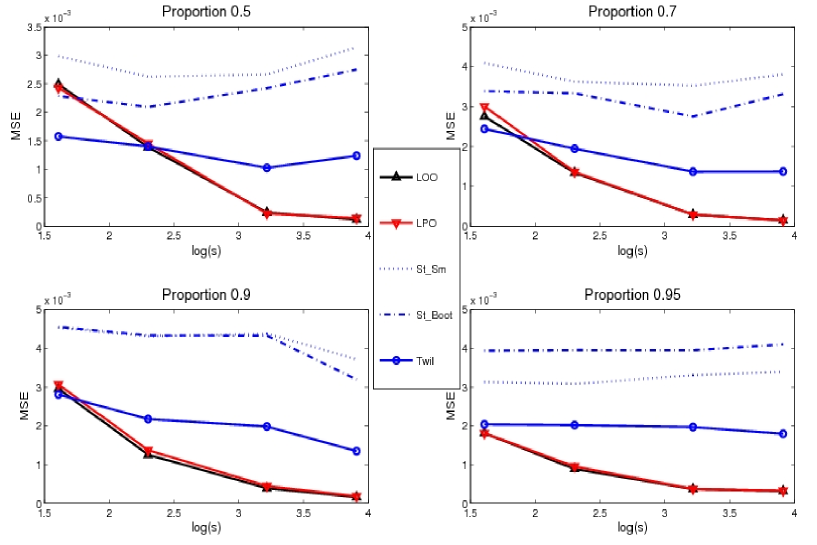
Figure 2: Graphs of the MSE of the $\pi_{0}$ estimator versus $\log s$, where $s$ is the parameter of the Beta density. Each graph is devoted to a given proportion, from 0.5 to 0.95 . $St_{Sm}$ denotes the MSE obtained for $Smoother$, $St_{Boot}$ that of $Bootstrap$ while $Twil$ states for $Twilight$.

Table 2: Numerical results for different $\pi_{0}$ estimators with $s=10$ and $\pi_{0}\in\{0.5,0.7,0.9,0.95\}$. Four other methods are compared to $LPO$ and $LOO$. $St_{Sm}$ denotes $Smoother$, $St_{Boot}$ states for $Bootstrap$ and $Twil$ for $Twilight.$(All displayed quantities are multiplied by 100.)

$\pi_{0}$ 0.5 0.7 Method Bias Std MSE Bias Std MSE $LPO$ 1.4 3.5 14.5 $10^{-2}$ 1.4 3.4 13.6 $10^{-2}$ $LOO$ 1.6 3.4 13.9 $10^{-2}$ 1.6 3.3 13.4 $10^{-2}$ $St_{Sm}$ -0.9 5.1 26.2 $10^{-2}$ -0.9 6.0 36.2 $10^{-2}$ $St_{Boot}$ -2.3 4.0 20.9 $10^{-2}$ -3.3 4.7 33.3 $10^{-2}$ $Twil$ -1.0 3.6 14.0 $10^{-2}$ -1.5 4.2 19.4 $10^{-2}$ $ABH$ 37.9 8.3 15.0 0.27 2.4 7.6

$\pi_{0}$ 0.9 0.95 Method Bias Std MSE Bias Std MSE $LPO$ 0.8 3.6 13.7 $10^{-2}$ 0.5 3.1 9.5 $10^{-2}$ $LOO$ 1.0 3.4 12.5 $10^{-2}$ 0.7 2.9 8.9 $10^{-2}$ $St_{Sm}$ -0.5 6.6 43.1 $10^{-2}$ -1.0 5.5 30.8 $10^{-2}$ $St_{Boot}$ -3.7 5.4 43.4 $10^{-2}$ -3.7 5.1 39.6 $10^{-2}$ $Twil$ -1.6 4.4 21.8 $10^{-2}$ -1.6 4.2 20.2 $10^{-2}$ $ABH$ 9.8 0.4 95.5 $10^{-2}$ 4.9 0.1 24.1 $10^{-2}$

3.2 Comparison in the U-shape case

The ’U-shape case’ refers to the phenomenon underlined by Pounds et al. PC on a real data set made of Affymetrix ’pooled’ present-absent p-values (one p-value per probe set). We explore the behaviour of the preceding methods applied to p-values with similar distributions. In our simulation design, the sample is $m=1000$, while $\pi_{0}\in\{0.25,0.5,0.7,0.8,0.9\}$ and $n=200$ repetitions of each condition have been made.
Typically, the U-shape case appears when one-sided tests are made whereas the non-tested alternative is true. For example, suppose the test statistics are distributed as a three-component gaussian mixture model

$$\pi_{0}\,\mathcal{N}(0,2.5\>10^{-2})+\frac{1-\pi_{0}}{2}\left[\mathcal{N}(a,\theta^{2})+\mathcal{N}(b,\nu^{2})\right],$$ (12)

where $a<0$, $b>0$ and $\theta,\nu>0,$ corresponding to respectively non-induced, under-expressed and over-expressed genes. We want to test whether genes are over-expressed, that is $H_{0}:$ ’the mean equals 0” versus $H_{1}:$ ’the mean is positive’. A test statistic drawn from $\mathcal{N}(a,\theta^{2})$ (under-expressed gene) is more likely to have a larger p-value than those under $\mathcal{N}(b,\nu^{2})$, which correspond actually to over-expressed genes. This phenomenon is clearly all the more deep as the gap between $a$ and $b$ is high and variances $\theta^{2}$ and $\nu^{2}$ are small. Note that a similar shape may be observed when test statistics are ill-chosen.
In order to mimic Pounds’ example, we use (12) with $-a=b\in\{1,1.5\}$ and $\theta=\nu\in\{0.5,0.75\}.$ As they were quite similar, results in these different conditions are gathered in Table 3.

Table 3: Results of the U-shape case for the six compared methods for $\pi_{0}\in\{0.25,0.5,0.7,0.8,0.9\}.$(All displayed quantities are multiplied by 100.)

$\pi_{0}$ 0.25 0.5 0.7 Method Bias Std MSE Bias Std MSE Bias Std MSE $LPO$ 5.5 6.2 0.7 5.5 5.2 0.6 5.3 4.4 0.5 $LOO$ 6.2 5.7 0.7 6.8 5.7 0.8 6.6 4.8 0.7 $St\_{Sm}$ 75.0 0 56.0 50.0 0 25.0 30.0 0 9.0 $St\_{Bo}$ 43.2 3.2 18.7 28.9 2.2 8.4 17.4 1.6 3.0 $Twil$ 73.2 2.5 53.6 47.5 3.0 22.6 27.4 2.3 8.0 $ABH$ 45.5 5.4 21.0 31.4 4.2 10.0 19.8 3.1 4.0

$\pi_{0}$ 0.8 0.9 Method Bias Std MSE Bias Std MSE $LPO$ 5.3 4.1 0.4 4.2 2.7 0.2 $LOO$ 6.4 4.1 0.6 4.7 2.5 0.3 $St\_{Sm}$ 20.0 0 4.0 9.9 0.2 1.0 $St\_{Bo}$ 11.6 1.3 1.0 5.4 1.6 0.3 $Twil$ 17.5 1.8 3.0 8.0 1.3 0.7 $ABH$ 13.8 2.3 2.0 7.4 1.3 0.6

Except $LPO$ and $LOO$ for which this phenomenon is not so strong, any other method all the more overestimates $\pi_{0}$ as the proportion of p-values under the uniform distribution is small. In our framework, a growth in $\pi_{0}$ entails an increase in the right part of the histogram near 1, which is responsible for the overestimation (violation of assumption (A)). On the contrary when $\pi_{0}=0.9$, the violation of assumption (A)) is weaker and similar values of MSE are obtained for the competing approaches. In this set-up, $LPO$, $LOO$ and $St_{Boot}$ provide systematically the lowest MSE values. In comparison, it is somewhat surprising that $Twilight$ overestimates $\pi_{0}$ so much, since it should have remained reliable under assumption (A’). Despite the preceding simulation results, we observe a repeated overestimation, which means that the criterion under-penalizes large sets of p-values. The involved penalty may have been designed for the situation before (with only one peak near 0), whereas it may be no longer relevant in this framework. This may be interpreted as a consequence of the higher adaptivity of cross-validation based methods over penalized criteria. Finally it is worth noticing that both the bias and the MSE of $LPO$ are systematically lower than those of $LOO$, showing the interest of choosing $p$ in an adaptive way.

3.3 Power

Here, we study the influence of the estimation of $\pi_{0}$ on the power of multiple testing procedures obtained as described in Section 3.1.2 for various $\pi_{0}$ estimators. The $Twilight$ method is used for comparison, in association with the Benjamini-Hochberg procedure (BH ). Our reference is what we call the Oracle procedure, which consists in plugging the true value of $\pi_{0}$ in the MTP procedure of Section 3.1.2. The same simulations as in Section 3.1.2 are used for this study, which is carried out in two steps. In the first one, we compare procedures in terms of their empirical $FDR$, in order to assess the expected control for finite samples. Thus, we choose the level $\alpha=0.15$ at which we want to control the $FDR$ and then compute, for each of the $n=500$ samples, the corresponding $FDP$ in the terminology of GW04 , e.g. the ratio of the number of falsely rejected hypotheses over the total number of rejections. Finally, we get an estimator of the actual $FDR$: $\widehat{FDR}$ by averaging the simulation results. Table 4 gives results for the LPO and LOO based procedures $\widehat{FDR}_{LPO}$, $\widehat{FDR}_{LOO}$ and also for $Twilight$ ($\widehat{FDR}_{Twil}$), Benjamini-Hochberg ($\widehat{FDR}_{BH}$) and Oracle procedures ($\widehat{FDR}_{Best}$). In the second step, we check the potential improvement in power enabled by the LPO-based MTP with respect to the BH-procedure. The assessment of this point is made in terms of the expectation of the proportion of falsely non-rejected hypotheses among true alternatives (named $FNR$ here). This criterion is estimated by the average of the preceding ratio computed from each sample. Table 5 displays the empirical $FNR$ values, denoted by $\widehat{FNR}_{LPO}$, $\widehat{FNR}_{LOO}$, $\widehat{FNR}_{Twil}$, $\widehat{FNR}_{BH}$ and $\widehat{FNR}_{Best}$ respectively for the LPO, LOO, $Twilight$, Benjamini-Hochberg and Oracle procedures. In both steps of this study, $s$ denotes the parameter of the Beta distribution that was used to simulate the data.

Table 4: Values of the empirical estimate of the FDR (%) for the LPO ($\widehat{FDR}_{LPO}$), LOO ($\widehat{FDR}_{LOO}$), $Twilight$ ($\widehat{FDR}_{Twil}$), Benjamini-Hochberg ($\widehat{FDR}_{BH}$) and Oracle ($\widehat{FDR}_{Best}$) procedures. $s$ denotes the parameter of the Beta distribution used to generate the data.

s	$\pi_{0}$	$\widehat{FDR}_{LPO}$	$\widehat{FDR}_{LOO}$	$\widehat{FDR}_{Twil}$	$\widehat{FDR}_{BH}$	$\widehat{FDR}_{Best}$
5	0.5	14.15	14.06	14.85	8.35	14.29
	0.7	14.13	14.03	14.85	10.40	14.50
	0.9	15.01	15.01	15.73	14.26	14.81
	0.95	13.23	13.43	13.76	13.13	13.83
10	0.5	14.74	14.69	15.50	6.94	15.02
	0.7	15.14	15.09	15.61	10.29	15.12
	0.9	17.91	17.90	18.08	15.85	17.94
	0.95	14.65	14.65	15.25	14.37	14.95
25	0.5	14.88	14.82	15.51	7.48	15.04
	0.7	14.69	14.64	15.19	10.47	14.84
	0.9	15.50	15.57	16.31	13.56	15.92
	0.95	14.35	14.22	14.51	13.19	14.19
50	0.5	14.76	14.71	15.42	7.40	14.89
	0.7	14.81	14.77	15.23	10.36	14.87
	0.9	13.93	13.82	14.79	13.17	13.98
	0.95	16.12	16.32	16.57	14.65	16.08

Table 5: Average proportion of falsely non-rejected hypotheses (%) for the LPO ($\widehat{FNR}_{LPO}$), LOO ($\widehat{FNR}_{LOO}$), $Twilight$ ($\widehat{FNR}_{Twil}$), Benjamini-Hochberg ($\widehat{FNR}_{BH}$) and Oracle ($\widehat{FNR}_{Best}$) procedures. $s$ denotes the parameter of the Beta distribution used to generate the data.

s	$\pi_{0}$	$\widehat{FNR}_{LPO}$	$\widehat{FNR}_{LOO}$	$\widehat{FNR}_{Twil}$	$\widehat{FNR}_{BH}$	$\widehat{FNR}_{Best}$
5	0.5	93.94	94.22	91.64	99.78	94.16
	0.7	99.65	99.65	99.59	99.80	99.63
	0.9	99.87	99.87	99.86	99.89	99.86
	0.95	99.91	99.91	99.90	99.92	99.91
10	0.5	25.69	25.91	22.01	96.83	23.22
	0.7	96.36	96.44	95.08	99.16	96.03
	0.9	99.56	99.56	99.54	99.64	99.56
	0.95	99.76	99.76	99.76	99.77	99.74
25	0.5	0.88	0.90	0.70	17.72	0.79
	0.7	22.83	23.04	20.85	61.00	21.93
	0.9	97.89	97.89	97.68	98.49	97.86
	0.95	99.16	99.16	99.06	99.23	99.14
50	0.5	0.96	0.92	0.64	1.58	0.72
	0.7	2.26	2.30	2.01	10.07	2.19
	0.9	82.40	82.47	80.39	88.05	82.08
	0.95	96.74	96.76	96.60	97.15	96.74

In comparison to the Oracle procedure (with the true $\pi_{0}$), Table 4 shows that the LPO procedure provides an actual value of the FDR that is almost always very close to the best possible one. Moreover in nearly all conditions, LPO outperforms its LOO counterpart and remains a little bit conservative, e.g. it furnishes a FDR that is lower or equal to the desired level $\alpha$. This observation empirically confirms the result stated in Theorem 2.2. Besides as expected, the estimation of $\pi_{0}$ entails a tighter control than that of the BH-procedure where $\widehat{\pi}_{0}=1$. Unlike the proposed methods, $Twilight$ fails in controlling the FDR at the desired level since $\widehat{FDR}_{Twil}$ is very often larger than $\widehat{FDR}_{Best}$ (the best reachable value), and even larger than $\alpha$. Subsequently, $Twilight$ should not enter in the comparison of methods in terms of power.
Table 5 enlightens that proportions of false negatives may be very high in most of the simulation conditions, as shown by the Oracle procedure. Nevertheless, $\widehat{FNR}_{LPO}$ remains very close to the ideal one. As a remark, note that the $Twilight$ FNR estimates are also close to the Oracle values, but nearly always lower. As suggested by FDR results, LOO is less powerful that LPO, whereas both of them outperform by far the BH-procedure. Note that the proportion of false negatives strongly decreases when $s$ grows, which means that ${\bf H}_{1}$ p-values are more and more concentrated in the neighbourhood of 0. As the interval on which assumption (A) is satisfied is wider, the problem becomes easier. Besides, we observe a fall in power when $\pi_{0}$ grows in general. Indeed for small proportion of true alternatives, the ”border” between the two populations of p-values is more difficult to define as a large number of ${\bf H}_{1}$ p-values behave like ${\bf H}_{0}$ ones. Finally note that very often, the LPO procedure shares (nearly) the same power as the Oracle one.

3.4 Discussion

In this article, we propose a new estimator of the unknown proportion of true null hypotheses $\pi_{0}$. It relies on first the estimation of the common density of p-values by use of non-regular histograms of a special type, and secondly on the leave-$p$-out cross-validation. The resulting estimator enables more flexibility than numerous existing ones, since at least it is still convenient in the ”U-shape” case, without any supplementary computational cost.
Our estimator may be linked with that of Schweder and Spjøtvoll for which almost only theoretical results with $\lambda$ fixed have been obtained by Storey. However unlike the latter, we provide a fully adaptive procedure that does not depend on any user-specified parameter. Thus, asymptotic optimality results are here derived with $\lambda=\widehat{\lambda}$. They assert, for instance, that the asymptotic exact control of the FDR with our plug-in MTP is reached.
Eventually, a wide range of simulations enlighten that the proposed $\pi_{0}$ estimator realizes the best bias-variance tradeoff among all tested estimates. Moreover, the proposed plug-in procedure is (empirically) shown to provide the expected control on the FDR (for finite samples), while being a little more powerful than its LOO counterpart. Moreover, the results in Section 3.2 confirm the interest in choosing adaptively the parameter $p$ rather than the usual $p=1$ value. The LPO procedure is very often almost as powerful as the best possible one of this type, obtained when $\pi_{0}$ is known.

4 Appendix

Proof.

(Lemma 2.5)
First, we show that $T(\alpha,\cdot,\widehat{G})$ is right (resp. left) continuous on $[0,1)$ (resp. $(0,1]$). As it is a similar reasoning, we only deal with right continuity.
Let $(\epsilon_{n})_{n}\in\left(\mathbb{R}_{+}^{*}\right)^{\mathbb{N}^{*}}$ denote a sequence decreasing towards 0. For any $\theta\in(0,1],$ set $\forall n,\ r_{n}=T(\alpha,\theta+\epsilon_{n},\widehat{G})\ a.s.\,.$ Then $(r_{n})_{n}$ is an almost surely convergent increasing sequence, upper bounded by $T(\alpha,\theta,\widehat{G})$. To prove that $T(\alpha,\theta,\widehat{G})$ is its limit, we show that for any $\delta>0,$ there exists $\epsilon>0$ satisfying $T(\alpha,\theta+\epsilon,\widehat{G})\geq T(\alpha,\theta,\widehat{G})-\delta.$ Notice that there exists $\eta>0$ s.t. $T:=T(\alpha,\theta,\widehat{G})=\sup\{t\in[\eta,1]:\,\widehat{Q}_{\theta}(t)\leq\alpha\}$. Then for $0<\delta<\eta,$ $T-\delta=\sup\left\{u\in[\eta-\delta,1-\delta]:\ \frac{\theta(u+\delta)}{\widehat{G}(u+\delta)}\leq\alpha\right\}.$ Provided $\delta$ is small enough, $\widehat{G}(u+\delta)=\widehat{G}(u),\ \forall u.$ Hence, $T-\delta=\sup\left\{u\in[\eta-\delta,1-\delta]:\ \frac{\theta u}{\widehat{G}(u)}+\frac{\theta\delta}{\widehat{G}(u)}\leq\alpha\right\},$ and $T(\alpha,\theta+\epsilon,\widehat{G})=\sup\left\{t\in[0,1]:\ \frac{\theta t}{\widehat{G}(t)}+\frac{\epsilon t}{\widehat{G}(t)}\leq\alpha\right\}.$ Thus, any $0<\epsilon<\delta\theta$ provides the result.
For the second point, define $G\in\mathcal{B}^{+}([0,1])$ and for any sequence $(\epsilon_{n})_{n}\in\left(\mathbb{R}_{+}^{*}\right)^{\mathbb{N}}$ decreasing towards 0, let $(H_{n})_{n}\in\left(\mathcal{B}^{+}([0,1])\right)^{\mathbb{N}}$ denote a sequence of positive bounded functions satisfying $\forall n,\ ||G-H_{n}||_{\infty}\leq\epsilon_{n}$. Then for large enough $n$, we have

$$\frac{\theta t}{G(t)-\epsilon_{n}}\leq\alpha \Leftrightarrow \frac{\theta t}{G(t)}\leq\alpha\left(1-\frac{\epsilon_{n}}{G(t)}\right),$$

and $\alpha(1-\epsilon_{n}/||G||_{\infty})\leq\alpha$. Thus, $r_{n}=\sup\{t:\ \theta t/(G(t)+\epsilon_{n})\leq\alpha\}$ denotes an increasing sequence that is bounded by $T(\alpha,\theta,G)$. Moreover as $(\epsilon_{n})_{n}$ decreases towards 0, $r_{n}$ is as close as we want to $T(\alpha,\theta,G)$. The same reasoning may be followed with $r^{\prime}_{n}=\sup\{t:\ \theta t/(G(t)-\epsilon_{n})\leq\alpha\},$ which concludes the proof. ∎

References

- [1] A. Barron, L. Birgé, and P. Massart. Risk bounds for model selection via penalization. Probab. Theory and Relat. Fields, 113:301–413, 1999.
- [2] P. L. Bartlett, S. Boucheron, and G. Lugosi. Model selection and error estimation. In Proceedings of the Thirteenth Annual Conference on Computational Learning Theory, pages 286–297, 2000.
- [3] Y. Benjamini and Y. Hochberg. Controlling the False Discovery Rate: a Practical and Powerful Approach to Multiple Testing. J.R.S.S. B, 57(1):289–300, 1995.
- [4] Y. Benjamini, A. M. Krieger, and D. Yekutieli. Adaptive Linear Step-up Procedures that control the False Discovery Rate. Biometrika, 93(3):491–507, 2006.
- [5] Y. Benjamini and D. Yekutieli. The control of the false discovery rate in multipe testing under dependency. The Annals of Statistics, 29(4):1165–1188, 2001.
- [6] P. Broberg. A comparative review of estimates of the proportion unchanged genes and the false discovery rate. BMC Bioinformatics, 6:199, 2005.
- [7] A. Celisse and S. Robin. Nonparametric density estimation by exact leave-p-out cross-validation. Computational Statistics and Data Analysis, doi:10.1016/j.csda.2007.10.002, 2007.
- [8] S. Dudoit, J. Popper Shaffer, and J. C. Boldrick. Multiple Hypothesis Testing in Microarray Experiments. Statistical Science, 18(1):71–103, 2003.
- [9] B. Efron. Large-Scale Simultaneous Hypothesis Testing: the choice of a null hypothesis. Journal of the American Statistical Association, 99(465):96–104, 2004.
- [10] B. Efron, R. Tibshirani, J. D. Storey, and V. Tusher. Empirical Bayes Analysis of a Microarray Experiment. Journal of American Statistical Association, 96(456):1151–1160, 2001.
- [11] C. Genovese and L. Wasserman. A stochastic process approach to false discovery control. The Annals of Statistics, 32(3):1035–1061, 2004.
- [12] U. Grenander. On the theory of mortality measurement. Skandinavisk Aktuarietidskrift, 39(2):125–153, 1956.
- [13] T. Hastie, R. Tibshirani, and J. Friedman. The Elements of Statistcal Learning. Springer Series in Statistics. Springer, 2001.
- [14] M. Kearns, Y. Mansour, A. Y. Ng, and D. Ron. A Experimental and Teoretical Comparison of Model Selection Methods. Machine Learning, 27:7–50, 1997.
- [15] M. Langaas, B. H. Lindqvist, and E. ferkingstad. Estimating the proportion of true null hypotheses, with application to DNA microarray data. J.R.S.S. B, 67(4):555–572, 2005.
- [16] E. Lebarbier. Detcting multiple change-points in the mean of Gaussian process by model selection. Signal Processing, 85:717–736, 2005.
- [17] S. Pounds and C. Cheng. Robust estimation of the false discovery rate. Bioinformatics, 22(16):1979–1987, 2006.
- [18] M. Rudemo. Empirical Choice of Histograms and Kernel Density Estimators. Scand. J. Statist., 9:65–78, 1982.
- [19] S. Scheid and R. Spang. A Stochastic Downhill Search Algorithm for Estimating the Local False Discovery Rate. I.E.E.E. Transactions on Computational Biology and Bioinformatics, 1(3):98–108, 2004.
- [20] S. Scheid and R. Spang. Twilight; a Bioconductor package for estimating the local false discovery rate. Bioinformatics, 21(12):2921–2922, 2005.
- [21] T. Schweder and E. Spjøtvoll. Plots of p-values to evaluate many tests simultaneously. Biometrika, 69:493–502, 1982.
- [22] D. Scott. On Optimal and Data-Based Histograms. Biometrika, 66(3):605–610, 1979.
- [23] J. Shao. Model Selection by Cross-Validation. Journal of the American Statis. Association, 88(422):486–494, 1993.
- [24] J. D. Storey. A direct approach to false discovery rates. J.R.S.S. B, 64(3):479–498, 2002.
- [25] J. D. Storey, J. E. Taylor, and D. Siegmund. Strong control, conservative point estimation and simultaneous conservative consistency of false discovery rates: a unified approach. J.R.S.S. B, 66(1):187–205, 2004.
- [26] J. D. Storey and R. Tibshirani. Statistical significance for genomewide studies. PNAS, 100(16):9440–9445, 2003.
- [27] A. W. van der Vaart. Asymptotic Statistics. Cambridge Series in Statistical and Probabilistic Mathematics. Cambridge University Press, 1998.
- [28] Y. Yang. Consistency of cross validation for comparing regression procedures. Annals of Statistics, Accepted paper.