KUNS-2133, UTAP-595, RESCEU-6/08, IPMU-08-0016

Decaying D-branes and Moving Mirrors
Tomoyoshi Hirata^a, Shinji Mukohyama^b,c and Tadashi Takayanagi^a

^a Department of Physics, Kyoto University, Kyoto 606-8502, Japan

^b Department of Physics and Research Center for the Early Universe, University of Tokyo, Tokyo, 113-0033, Japan

^c Institute for the Physics and Mathematics of the Universe, University of Tokyo, Chiba 277-8568, Japan

We present an exact time-dependent solution to the effective D-brane world-volume theory which describes an inhomogeneous decay of a brane-antibrane system. We compute the quantum energy flux induced by the particle creation in this inhomogeneous and time-dependent background. We find that this calculation is essentially equivalent to that of the moving mirror system. In the initial stage, the energy flux turns out to be thermal with the temperature given by the inverse of the distance between the brane and the antibrane. Later it changes its sign and becomes a negative energy flux. Our result may be relevant for the (p)reheating process or/and the evolution of cosmic string network after stringy brane inflation.

1 Introduction

The brane-antibrane system [1] has been studied intensively until recently as a typical example of unstable non-supersymmetric systems in string theory [2]. When a brane and an antibrane are close to each other, the open string spectrum includes tachyons. The condensation of open string tachyons offers us an important time-dependent background.

When the distance between a brane and an antibrane is larger than the string scale, there exits no tachyon. However, by an instanton effect or a small dynamical perturbation induced by collisions with other objects, it is possible that the distance between them becomes the string scale at a particular region or a point. In this setup, we expect that there exists a localized open string tachyon and the tachyon condensation occurs only in that region. This leads to a recombination of the brane and antibrane. Once this happens, this system annihilates via the time evolution and eventually the whole system will disappear radiating closed strings. However, the study in this direction has been rather few even at present.

The brane-antibrane system plays important roles not only in theoretical foundations of string theory but also in its cosmological applications. (See ref. [3] and references therein for a recent review of string cosmology.) Indeed, a string theoretic realization of hybrid inflation, called warped brane inflation [4], was made possible by non-trivial dynamics of the brane-antibrane system. In this scenario, the distance between a brane and an antibrane embedded in a warped geometry plays the role of inflaton. Our $4$-dimensional universe parallel to the world-volume of the brane-antibrane system expands with an accelerated expansion rate while the interbrane distance slowly decreases [5]. When the interbrane distance becomes as short as the local string length, a tachyon appears and starts rolling. This process of brane-antibrane annihilation releases sufficient energy to reheat our universe and starts the hot big-bang cosmology.

In hybrid inflation in field theory [6, 7], the reheating process begins with the so called tachyonic preheating [8]. This highly non-linear, inhomogeneous dynamical process occurs due to the tachyonic instability near the top of the water-fall potential. The tachyonic instability converts most of the energy into that of colliding classical waves very rapidly, within a single oscillation. The tachyonic preheating is a typical example of processes in which inhomogeneities are crucial.

As in the tachyonic preheating of the field-theoretic hybrid inflation, inhomogeneities are expected to play essential roles also in the reheating process of the warped brane inflation. In view of this, the brane-antibrane annihilation should begin locally in regions where the interbrane distance reaches the string length earlier than the other parts, and those regions should turn into “expanding holes“ on the world-volume of the brane-antibrane system. The whole annihilation process proceeds as those “expanding holes” collide with each other and percolate. Therefore, the study of inhomogeneous annihilation of brane-antibrane pair is an important subject towards our better understanding of the end of the brane inflation and the beginning of the thermal history of our universe.

Motivated by these, in this paper we would like to analyze the real time evolution of a brane-antibrane system after the local annihilation or recombination occurs (refer to [9] for an analysis of the process of the recombination). We first present a simple exact solution to the DBI action of D-branes which describes the time evolution of a brane-antibrane system. Then we will calculate the quantum energy flux produced by the open string creation. In particular, we will mainly focus on the brane-antibrane system of a D-string and an anti D-string (i.e. $D1-\overline{D1}$ system) for simplicity by a technical reason that we can apply the two dimensional conformal field theory. The argument of general Dp-branes can also be possible in principle and will not be essentially different. As we will show, our computation of energy flux has a close relation to the analysis of the moving mirror [10, 11]. Finally, we will interestingly notice that we encounter a negative energy flux in this process of decaying branes.

The inhomogeneous annihilation of D-string and anti D-string considered in this paper may be regarded as a lower-dimensional proto-type of the “expanding hole” mentioned above [12]. The process considered in this paper is probably relevant also for the dynamics of cosmic superstring network formed after the warped brane inflation. Indeed, the recombination of strings is one of the most important factors for the evolution of the cosmic superstring network. (See ref. [13] and references therein for a review of cosmic superstrings.)

This paper is organized as follows. In section two, we present an exact solution which describes the decay of brane-antibrane systems. In section three, we study the induced metric on this time-dependent world-volume of the decaying brane. In section four, we compute the energy flux in this process induced by the particle creation mechanism, relating this calculation to the one in the moving mirror system. We also discuss its string theoretic interpretations. In section five we summarize conclusions and discuss future problems.

2 Real Time Decay of D-string anti D-string Pair

Consider a parallel D-string anti D-string pair separated by a distance $d$. When $d>2\pi l_{s}$ in bosonic string (or $d>\sqrt{2}\pi l_{s}$ in superstring), the open string between the D-string and the anti D-string does not have any tachyonic modes ($l_{s}$ is the string length). Therefore in this case, the decay will be induced by their relative motion.

Even though we started with the system of a brane and an antibrane, we can regard the total system as a single D-string after the recombination occurs. Then we can describe the motion of the system by the DBI action of D-string as long as the stringy corrections are negligible.

2.1 Exact Solution of Time Evolution

We assume that the D-string is included within the $(2+1)$ dimensional hypersurface $R^{1,2}$, specified by the coordinate $(t,x,y)$ in the $D=10$ (or $D=26$) dimensional superstring (or bosonic string) theory. The profile of the D-string is described by the function $y=y(t,x)$. Then the Lagrangian of the DBI action for the D-string is written as follows

$$L=\sqrt{1-\dot{y}^{2}+y^{\prime 2},}$$ (2.1)

where $\dot{y}=\frac{\partial y}{\partial t}$ and $y^{\prime}=\frac{\partial y}{\partial x}$.

Let us find its solution by assuming the form $y(t,x)=f(x)+g(t)$. The equation of motion for (2.1) leads to

$$\ddot{g}(1+f^{\prime 2})+f^{\prime\prime}(\dot{g}^{2}-1)=0.$$ (2.2)

Thus we find $\frac{\ddot{g}}{1-\dot{g}^{2}}=\frac{f^{\prime\prime}}{1+f^{\prime 2}}=$const. This can be solved as follows

$$g(t)=\alpha\log\cosh\frac{t}{\alpha},\ \ \ \ \ f(x)=-\alpha\log\cos\frac{x}{\alpha}.$$ (2.3)

In this way we find the time-dependent solution

$$e^{y/\alpha}\cos(x/\alpha)=\cosh(t/\alpha),$$ (2.4)

where $x$ runs the range $-\frac{\pi}{2}\alpha\leq x\leq\frac{\pi}{2}\alpha$. Actually, its Euclidean version $e^{y/\alpha}\cos(x/\alpha)=\cos(z/\alpha)$ is known as the Scherk minimal surface in differential geometry.

This solution (2.4) represents a decay of a D-string and an anti D-string. Indeed, when $y$ is very large at a fixed time $t$, the coordinate $x$ approaches to either of two values $x=\pm\frac{\pi}{2}\alpha$. These two branches correspond to the D-string and the anti D-string separated by the distance $d=\pi\alpha$. Since we assume that there are no tachyons between them, we require $\alpha\gg l_{s}$. Notice also that $y$ satisfies $y\geq\alpha\log\cosh(t/\alpha)$ in (2.4). This means that this string pair is annihilated for $y\ll\alpha\log\cosh(t/\alpha)$. They are recombined at $y=\alpha\log\cosh(t/\alpha)$. In summary, this D-brane at a fixed time looks like a hairpin as described in the Fig.1.

Figure 1: The left figure shows the hairpin-like shape of the time-dependent D-string (2.4) at a fixed time $t$. The right one describes its time-dependence explicitly. The tip (or turning point) of the D-string is located at $x=0$ and its time evolution is given by $y(t)=\alpha\log\cosh(t/\alpha)$. This trajectory becomes light-like in the limit $t\to\pm\infty$.

The effective action of curved D-branes is described by the DBI action (2.1) only if we can neglect the higher derivative terms. This requires that the curvature of the induced metric is smaller than the string scale. As we will briefly discuss in the next section, such stringy corrections become important only if we consider the behavior near $t\to\pm\infty$ in the region close to the recombined point (or turning point) $x=0$. Thus the stringy corrections are not essential to our main results in this paper.

One may notice that another possible decay process is that the brane and the antibrane approach via the attractive force between them. A simple analysis estimates the life time due to this process as $\sim\frac{\alpha^{4}}{\sqrt{g_{s}}l_{s}^{3}}$. This is clearly much longer than the time scale $\alpha$ of our solution (2.4).

We can take into account the gauge field $A_{\mu}$ on the brane. A solution with an electric flux is shown in the in the appendix A. We can also generalize straightforwardly the above analysis to the systems of a Dp-brane and an anti Dp-brane by trivially adding extra coordinates. The profile (2.4) remains the same in this case. In these higher dimensional examples, there are also other decay modes such as making a hole leading to a wormhole like configuration as discussed in [12]. We leave the analysis of the time evolution of such configurations for an interesting future problem.

3 Induced Metric and Transverse Scalars

Open strings on the D-string probe the time dependence of the background via the time-dependent induced metric of the D-string

$$ds^{2}=-\frac{dt^{2}}{\cosh^{2}(t/\alpha)}+\frac{dx^{2}}{\cos^{2}(x/\alpha)}+2\tan(x/\alpha)\tanh(t/\alpha)dtdx.$$ (3.1)

3.1 Induced Metric in Conformal Gauge

It is useful to rewrite this metric into the one in the conformal gauge

$$ds^{2}=A(\tau,y)(-d\tau^{2}+dy^{2}),$$ (3.2)

so that the Lagrangian of minimally coupled massless scalar fields $\phi$ becomes simple at quadratic order

$$L=\frac{1}{2}\left(-(\partial_{\tau}\phi)^{2}+(\partial_{y}\phi)^{2})\right).$$ (3.3)

Requiring that the coordinate $y$ in (3.2) is the same as the one in (2.4), we find an appropriate coordinate transformation as follows

$$\tau = \alpha\log\left[\sqrt{1+\sinh^{2}(t/\alpha)\sin^{2}(x/\alpha)}+\sin(x/\alpha)\sinh(t/\alpha)\right],$$

$$y = \alpha\log\cosh(t/\alpha)-\alpha\log\cos(x/\alpha).$$ (3.4)

It is equivalent to the relation

$$\sinh(\tau/\alpha)=\sinh(t/\alpha)\sin(x/\alpha),\ \ \ \ \ \ \ \ e^{y/\alpha}=\frac{\cosh(t/\alpha)}{\cos(x/\alpha)}.$$ (3.5)

The metric in this coordinate system reads

$$ds^{2}=-\left(\frac{1}{2}+\frac{\cosh\frac{v-u}{2\alpha}}{2\sqrt{\sinh\frac{v}{\alpha}\cdot\sinh\frac{-u}{\alpha}}}\right)dudv,$$ (3.6)

where we defined

$$u=\tau-y,\ \ \ \ v=\tau+y.$$ (3.7)

We need to deal with the metric (3.6) carefully. It is well-defined for $y>|\tau|$. When we go beyond this bound, the coordinate $y$ (and $\tau$) in (3.6) becomes time-like (space-like) and we have to exchange $\tau$ with $y$ and vise versa, which is equal to the sign flip of $u$ and $v$. Also at the bound $y=\pm\tau$, the metric becomes singular. Actually, we can further perform a coordinate transformation and obtain a completely smooth metric which covers the total spacetime on the D-string as we show in the appendix B.

3.2 Asymptotically Flat Coordinate

The metric (3.6) at the null past infinity $u=-\infty$ approaches

$$A(u,\infty)=\frac{1}{2}\left(1+\frac{1}{\sqrt{1-e^{-2v/\alpha}}}\right).$$ (3.8)

On the other hand in the limit $v=\infty$ of the future null infinity we get

$$A(-\infty,v)=\frac{1}{2}\left(1+\frac{1}{\sqrt{1-e^{2u/\alpha}}}\right).$$ (3.9)

Thus we can define the asymptotically flat metric by the coordinate transformation

$$V=-\frac{\alpha}{2}\log(1-\sqrt{1-e^{-2v/\alpha}}),$$

$$U=\frac{\alpha}{2}\log(1-\sqrt{1-e^{2u/\alpha}}).$$ (3.10)

In terms of $(U,V)$, the metric $ds^{2}=-A(U,V)dUdV$ is found to be

$$\tilde{A}(U,V) = A(u,v)\frac{dv}{dV}\frac{du}{dU}$$

$$= \frac{2\left(1+e^{-V/\alpha}e^{U/\alpha}\sqrt{2-e^{-2V/\alpha}}\sqrt{2-e^{2U/\alpha}}+(1-e^{-2V/\alpha})(1-e^{2U/\alpha})\right)}{(2-e^{-2V/\alpha})(2-e^{2U/\alpha})}.$$

It is easy to see that this is manifestly asymptotically flat:

$$ds^{2}\simeq-dUdV$$ (3.12)

near the past null infinity ($U\to-\infty$) and the future null infinity ($V\to\infty$). This coordinate system is regular in the regime

$$V>-\frac{\alpha}{2}\ln 2,\quad U<\frac{\alpha}{2}\ln 2.$$ (3.13)

3.3 Global Geometry

In this coordinate $(U,V)$, the turning point $x=0$ is described by the curve

$$e^{\frac{-2V}{\alpha}}+e^{\frac{2U}{\alpha}}=2,$$ (3.14)

or

$$V=P(U),\quad P(U)\equiv-\frac{\alpha}{2}\ln\left(2-e^{2U/\alpha}\right).$$ (3.15)

The half of the D-string spacetime $x\geq 0$ is mapped to the region $V\geq P(U)$, while another half $x\leq 0$ is mapped to the region $U\geq P(V)$. Since they are actually equivalent by the reflection, the global geometry is obtained by gluing two copies of the region $V>P(U)$ along the symmetry axis $V=P(U)$ as in Fig.2. Note that both of them are included in the regime (3.13) of validity of the coordinates $(U,V)$. For more explanations of the global structure of our metric, see the appendix B.

Figure 2: The Penrose diagram of our time-dependent spacetime (3.2). $x\geq 0$ is mapped to region I, and $x\leq 0$ is mapped to region II. The global geometry can be obtained by gluing two shaded regions along the curve $x=0$ represented by the thick curve.

If we define $U=\bar{t}-\bar{y}$ and $V=\bar{t}+\bar{y}$, this curve is described by

$$\bar{y}=\frac{\alpha}{2}\log\cosh\frac{2\bar{t}}{\alpha}.$$ (3.16)

Notice that this curve is slightly off from the naive estimate $y\sim\alpha\log\cosh\frac{\bar{t}}{\alpha}$ from (2.4) by the factor 2. This is related to the fact that the value of the metric function $\tilde{A}$ on $V=P(U)$ is off from unity,

$$\tilde{A}(U,P(U))=4.$$ (3.17)

On the other hand, along the symmetry axis $dU$ and $dV$ are related as

$$dU=\frac{e^{-2V/\alpha}}{2-e^{-2V/\alpha}}dV.$$ (3.18)

Thus, the induced line element along the symmetry axis is

$$ds^{2}=-\frac{4e^{-2V/\alpha}}{2-e^{-2V/\alpha}}dV^{2}.$$ (3.19)

This shows that the symmetry axis $V=P(U)$ is asymptotically null in the limit $V/\alpha\to\infty$.

One can check that the extrinsic curvature of the symmetry axis vanishes so that the two copies of the region $V>P(U)$ are glued smoothly. For this purpose, let us introduce a unit normal vector $n^{a}$ as

$$n^{U}=-\frac{1}{\sqrt{\tilde{A}}}e^{-U/\alpha}e^{-V/\alpha},\quad n^{V}=\frac{1}{\sqrt{\tilde{A}}}e^{U/\alpha}e^{V/\alpha}.$$ (3.20)

The extrinsic curvature is defined as

$$K_{ab}=\left.\frac{1}{2}q_{a}^{\ c}q_{b}^{\ d}(\nabla_{c}n_{d}+\nabla_{d}n_{c})\right|_{V=P(U)},$$ (3.21)

where

$$q_{ab}=g_{ab}-n_{a}n_{b}.$$ (3.22)

By explicit calculation it is shown that

$$K_{ab}=0.$$ (3.23)

Therefore, two copies of the region $V>P(U)$ are glued smoothly as should be. Hereafter, we call one of the two copies of the region $V>P(U)$ the region I and the other the region II (see Fig.2.). In this way we get a completely smooth coordinate which covers the total spacetime.

Before we proceed, we would also like to examine stringy corrections which we neglected in this paper. In order to argue it is negligible, we need to require $l^{2}_{s}R_{\mu\nu\rho\sigma}^{(2)}\ll 1$ in the region I (the analysis of region II is the same). The curvature tensor takes larger values as we come close to the curve $V=P(U)$ and there it behaves like $R_{\mu\nu\rho\sigma}^{(2)}\sim\frac{1}{\alpha^{2}}e^{4V/\alpha}$. Therefore the condition of neglecting stringy corrections is given by

$$V\ll\frac{\alpha}{2}\log\frac{\alpha}{l_{s}}.$$ (3.24)

Since we assumed from the beginning $\alpha\gg l_{s}$, we can still neglect the stringy corrections even if we take $\frac{V}{\alpha}$ to be appropriately large.

3.4 Transverse Scalar as Tachyon

The main motivation of the above analysis of the induced metric is to understand the low energy effective action of open string modes. Since gauge fields in $1+1$ dimension are not dynamical, we would like to consider the transverse scalar fields. First we focus on the transverse scalars $\phi_{i}$ $(i=3,4,\cdot\cdot\cdot,D)$ which correspond to the deformations into the directions orthogonal to the $R^{1,2}$ defined by $(t,x,y)$. In the low energy limit, their effective actions are all equal to the one of the (minimally coupled) massless scalar field $L=\frac{1}{2}\sqrt{-g}g^{\mu\nu}\partial_{\mu}\phi\partial_{\nu}\phi$, where $\mu$ and $\nu$ run over the D-string world-volume and $g_{\mu\nu}$ is the induced metric of the D-string (3.2).

There is another transverse scalar which describes the motion of D-string within the $R^{1,2}$ spacetime. As shown in the appendix D, at the quadratic order, the effective action is given by the one of a massive scalar field $L=\frac{1}{2}\sqrt{-g}(g^{ab}\partial_{a}\phi\partial_{b}\phi+m^{2}\phi^{2})$ with the mass square given by

$$m^{2}=\frac{1}{2}(R^{(2)}-K^{\mu\nu}K_{\mu\nu}),$$ (3.25)

where $K_{\mu\nu}$ is the extrinsic curvature. It turns out that in our example of the decaying D-string and anti D-string the mass square becomes negative

$$m^{2}=-\frac{2\sec^{2}\frac{x}{\alpha}~{}\mbox{sech}^{2}\frac{t}{\alpha}}{\alpha^{2}(\sec^{2}\frac{x}{\alpha}~{}\mbox{sech}^{2}\frac{t}{\alpha}+\tan^{2}\frac{x}{\alpha}~{}\tanh^{2}\frac{t}{\alpha})^{2}}<0,$$ (3.26)

and therefore the scalar is a tachyonic mode. In this paper we restrict to the case where the condensation of this tachyon does not occur. It is a quite interesting future problem to see what will happen if the tachyon condenses.

4 Energy Flux from Decaying D-brane

Now we move on to the main part of this paper. We would like to analyze the particle creation (open string creation) in the time-dependent open string theory on the D-string (2.4). As we will mention, this analysis is essentially the same as that of moving mirror systems. First we concentrate on massless transverse scalars and later we will discuss the result when we take all stringy modes into account.

4.1 Energy Flux in Massless Scalar Theory

We introduce a minimally-coupled, massless scalar field $\phi$. By decomposing the field into left- and right-moving parts as

$$\phi=\left\{\begin{array}[]{ll}\phi_{I+}(V)+\phi_{I-}(U)&(\mbox{region I})\\ \phi_{II+}(V)+\phi_{II-}(U)&(\mbox{region II})\\ \end{array}\right.,$$ (4.1)

the smoothness of the field implies that

$$\phi_{I-}(U)=\phi_{II+}(P(U)),\quad\phi_{II-}(U)=\phi_{I+}(P(U)).$$ (4.2)

Thus, we obtain a general solution

$$\phi=\left\{\begin{array}[]{ll}\phi_{I+}(V)+\phi_{II+}(P(U))&(\mbox{region I})\\ \phi_{II+}(V)+\phi_{I+}(P(U))&(\mbox{region II})\\ \end{array}\right..$$ (4.3)

We consider the vacuum $|in\rangle$ defined by the following mode functions

$$\phi^{(L)}=\left\{\begin{array}[]{ll}\frac{1}{\sqrt{4\pi\omega}}e^{-i\omega V}&(\mbox{region I})\\ \frac{1}{\sqrt{4\pi\omega}}e^{-i\omega P(U)}&(\mbox{region II})\\ \end{array}\right.,$$ (4.6)

$$\phi^{(R)}=\left\{\begin{array}[]{ll}\frac{1}{\sqrt{4\pi\omega}}e^{-i\omega P(U)}&(\mbox{region I})\\ \frac{1}{\sqrt{4\pi\omega}}e^{-i\omega V}&(\mbox{region II})\\ \end{array}\right..$$ (4.9)

The Weightman function in each region is

$$G(x,x^{\prime}) \equiv \langle in|\phi(x)\phi(x^{\prime})|in\rangle$$ (4.10)

$$= \int_{0}^{\infty}d\omega\left[\phi^{(L)}_{i\omega}(x)\phi^{(L)*}_{i\omega}(x^{\prime})+\phi^{(R)}_{i\omega}(x)\phi^{(R)*}_{i\omega}(x^{\prime})\right]$$

$$= G^{(0)}(x,x^{\prime})+\Delta G(x,x^{\prime}),$$

where

$$G^{(0)}(x,x^{\prime})\equiv\int_{0}^{\infty}\frac{d\omega}{4\pi\omega}\left[e^{-i\omega(V-V^{\prime})}+e^{-i\omega(U-U^{\prime})}\right],$$ (4.11)

and

$$\Delta G(x,x^{\prime}) \equiv G(x,x^{\prime})-G^{(0)}(x,x^{\prime})$$ (4.12)

$$= \int_{0}^{\infty}\frac{d\omega}{4\pi\omega}\left(e^{-i\omega(P(U)-P(U^{\prime}))}-e^{-i\omega(U-U^{\prime})}\right)$$

$$= \frac{1}{4\pi}\ln\left[\frac{U-U^{\prime}+i\epsilon}{P(U)-P(U^{\prime})+i\epsilon}\right].$$

Here, to obtain the last line, we have used

$$\int_{0}^{\infty}\frac{d\omega}{\omega}\left(e^{i\omega x}-e^{i\omega y}\right)=\ln\left(\frac{y-i\epsilon}{x-i\epsilon}\right).$$ (4.13)

Thus, the renormalized stress-energy tensor for each field for the state $|in\rangle$ is decomposed as

$$T^{(ren)}_{ab}=T^{(0)}_{ab}+\Delta T_{ab},$$ (4.14)

where $T^{(0)}_{ab}$ is the contribution from $G^{(0)}$ obtained later and $\Delta T_{ab}$ is the contribution from $\Delta G$ given by

$$\Delta T_{UU} = \lim_{x^{\prime}\to x}\partial_{U}\partial_{U^{\prime}}\Delta G(x,x^{\prime})=-\frac{1}{24\pi}\left\{P(U),U\right\},$$

$$\Delta T_{VV} = \lim_{x^{\prime}\to x}\partial_{V}\partial_{V^{\prime}}\Delta G(x,x^{\prime})=0,$$

$$\Delta T_{UV} = \Delta T_{VU}=0.$$ (4.15)

where $\{f,z\}$ is the Schwarzian derivative defined by

$$\{f,z\}=-2\sqrt{df/dz}\frac{d^{2}}{dz^{2}}\left(\frac{1}{\sqrt{df/dz}}\right),$$ (4.16)

and satisfies

$$\left(\frac{f(z_{2})-f(z_{1})}{x_{2}-x_{1}}\right)^{2}\frac{1}{f^{\prime}(z_{1})f^{\prime}(z_{2})}=1-\frac{1}{6}\left\{f,z\right\}(z_{2}-z_{1})^{2}+O(z_{2}-z_{1})^{4}.$$ (4.17)

The contribution $T^{(0)}_{ab}$ from $G^{(0)}(x,x^{\prime})$ can be obtained by properly subtracting divergent parts, differentiating with respect to $x$ and $x^{\prime}$ and taking the coincident limit. The result must be local in the sense that all components are functions of the metric function $\tilde{A}$ and its derivatives. In particular, they must be independent of the function $P(U)$. Moreover, $T^{(0)}_{ab}$ must vanish in the asymptotically flat region since the subtracted divergent parts are local geometric functions.

Actually, all components of $T^{(0)}_{ab}$ can be determined by the following three conditions: (i) it satisfies the conservation equation $\nabla^{a}T^{(0)}_{ab}=0$; (ii) its trace is determined by the trace anomaly $T^{(0)a}_{\ a}=R/(24\pi)$, where $R=4\tilde{A}^{-3}[\tilde{A}\partial_{U}\partial_{V}\tilde{A}-(\partial_{U}\tilde{A})(\partial_{V}\tilde{A})]$ is the Ricci scalar; (iii) it vanishes in the asymptotically flat region. The general solution to the conditions (i) and (ii) is

$$T^{(0)}_{UU} = -\frac{1}{12\pi}\sqrt{\tilde{A}}\partial_{U}^{2}\left(\frac{1}{\sqrt{\tilde{A}}}\right)+\alpha(U),$$

$$T^{(0)}_{VV} = -\frac{1}{12\pi}\sqrt{\tilde{A}}\partial_{V}^{2}\left(\frac{1}{\sqrt{\tilde{A}}}\right)+\beta(V),$$

$$T^{(0)}_{UV} = T^{(0)}_{VU}=-\frac{\tilde{A}}{96\pi}R,$$ (4.18)

where $\alpha(U)$ and $\beta(V)$ are arbitrary functions. Finally, the condition (iii) implies that

$$\alpha(U)=0,\quad\beta(V)=0.$$ (4.19)

In summary, we obtain

$$T^{(ren)}_{UU} = -\frac{1}{12\pi}\sqrt{\tilde{A}}\partial_{U}^{2}\left(\frac{1}{\sqrt{\tilde{A}}}\right)+\Delta T_{UU},$$

$$T^{(ren)}_{VV} = -\frac{1}{12\pi}\sqrt{\tilde{A}}\partial_{V}^{2}\left(\frac{1}{\sqrt{\tilde{A}}}\right),$$

$$T^{(ren)}_{UV} = T^{(0)}_{VU}=\frac{1}{24\pi\tilde{A}^{2}}\left[(\partial_{U}\tilde{A})(\partial_{V}\tilde{A})-\tilde{A}\partial_{U}\partial_{V}\tilde{A}\right],$$ (4.20)

where

$$\Delta T_{UU}=-\frac{1}{24\pi}\left\{P(U),U\right\}.$$ (4.21)

In the asymptotically flat region, only $\Delta T_{UU}$ is relevant:

$$T^{(ren)}_{UU} \to \Delta T_{UU},$$

$$T^{(ren)}_{VV} \to 0,$$

$$T^{(ren)}_{UV} = T^{(0)}_{VU}\to 0.$$ (4.22)

For $P(U)$ in (3.15), the Schwarzian derivative is

$$\left\{P(U),U\right\}=-\frac{8}{\alpha^{2}}\frac{1-e^{2U/\alpha}}{(2-e^{2U/\alpha})^{2}}.$$ (4.23)

Thus, we obtain

$$\Delta T_{UU}=\frac{1}{3\pi\alpha^{2}}\frac{1-e^{2U/\alpha}}{(2-e^{2U/\alpha})^{2}}.$$ (4.24)

Notice that this energy flux (4.24) approaches the following constant in the limit $U\to-\infty$

$$\Delta T_{UU}\to\frac{1}{12\pi\alpha^{2}}\equiv\frac{\pi}{12}T_{D}^{2}.$$ (4.25)

This suggests that a static detector will observe the thermal flux at the temperature $T_{D}=\frac{1}{\pi\alpha}$ long before it will collides with the tip of the D-string (i.e. $x=0$). This can be more clearly confirmed by computing the Bogolubov coefficients as we do in the appendix C.

However, later it gradually decreases and eventually changes its sign (i.e. negative flux) as described in Fig.3. In the end the detector collides with the tip of D-string. Thus the negative flux is observed only for a finite time $\Delta t=\frac{\alpha}{2}\log 2$.

It even gets negatively divergent precisely when it collides with the tip of the D-string at $U=\frac{\alpha}{2}\log 2$ if we literally accept (4.24). However, we have to remember that the string corrections become important when the condition (3.24) is violated. Indeed, if we assume $V\sim\frac{\alpha}{2}\log\frac{\alpha}{l_{s}}$, we find that the energy density becomes of the same order as the fundamental string tension $\Delta T_{UU}\sim\frac{1}{l^{2}_{s}}$. Therefore when this divergence happens the stringy corrections cannot already be negligible and they will plausibly give substantial modifications.

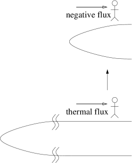
Figure 3: The behavior of the energy flux due to the particle creation under time evolution. In the left figure we show the spacetime regions where the sign of the energy flux is $+$ or $-$. A detector which is far from the tip of the brane first observes a thermal energy flux. However, later it changes into a negative energy flux and finally collides with the end point. This is summarized in the right figure.

4.2 D-brane Interpretation and Moving Mirror

Now we would like to interpret the above result from the viewpoint of the decay of the D-string-anti D-string system. Before the decay occurs, the effective world volume theory of the system at low energy is regarded as a $1+1$ dimensional $U(1)\times U(1)$ gauge theory. Concentrating on a massless scalar in this theory, the ones for the brane and antibrane are denoted by $\phi_{I}(t,y)$ and $\phi_{II}(t,y)$. Here notice that we considered that the fields on the D-brane and the anti D-brane live in the same $1+1$ dimensional spacetime assuming that the distance between the D-branes is much smaller than the typical length scale which the observer probes.

After the time evolution (2.4) starts, the brane and anti-brane become connected at a point $y=y_{*}(t)$ and the $U(1)\times U(1)$ gauge symmetry is broken there. The continuity of the scalar fields at $y=y_{*}(t)$ requires the following boundary conditions

$$\phi_{I}(t,y_{*}(t))-\phi_{II}(t,y_{*}(t))=0,\ \ \ \ \left.n^{a}\partial_{a}\left[\phi_{I}(t,y)+\phi_{II}(t,y)\right]\right|_{y=y_{*}(t)}=0,$$ (4.26)

where $n^{a}$ is a unit normal to the curve $y=y_{*}(t)$. Taking the global metric, the function $y_{*}(t)$ in our case is explicitly given by (3.16).

In our global geometry, the massless particle which propagates in the $x<0$ (or $x>0$) region ”reflects” at $y=y_{*}(t)$, and then comes into the $x>0$ (or $x<0$) region. Thus we can consider the trajectory $y=y_{x}(t)$ as a perfect ”mirror” in the $1+1$ dimensional space-time, and this setup is essentially the same as the one of the moving mirror system in which boundary conditions depend on time (see e.g.[10, 11]).

In general situations, when the mirror is moving at a non-zero acceleration, the static observer detects the thermal flux by the Unruh effect. It is described by a quantum field theory in the presence of the time-dependent boundary condition. For example, the Hawking radiation from a Schwarzschild black hole can also be regarded as a particular setup of moving mirror defined by $y(t)=-t-e^{-2\pi T_{bh}t}$, where $T_{bh}$ is the Hawking temperature of the black hole. A similar analysis of the energy flux $\Delta T_{UU}$ in section 3.1 and of the Bogolubov coefficients in the appendix C, correctly reproduces the well-known properties of the Hawking radiation [10].

Indeed, our boundary conditions (4.26) are equivalent to the moving mirror system with two massless scalars. One of the two scalars obeys the Dirichlet boundary condition and the other does the Neumann one. Therefore, the energy flux in the low energy world volume theory of the brane-antibrane system should be identified with the twice of (4.24). If we consider other massless fields, assuming the conformal invariance, we just need to multiply the value of central charge $c$ with (4.25).

In the actual open string theory, there are infinitely many massive fields in the brane-antibrane system in addition to the massless fields we discussed. Let us try to take all stringy massive modes into account in our argument of particle creation. Notice also that if we are interested in higher dimensional Dp-branes ($p>1$) case, we can regard the transverse momenta as the Kaluza-Klein momenta, generating extra mass terms. Therefore the treatment of decaying Dp-branes is similar. Unfortunately, even in two dimension, an exact analysis of a massive scalar field in the moving mirror setup is not available at present. Still we can roughly estimate the total energy flux as follows.

We consider the open string creation long before the observer collides with the tip of the brane. The result (4.24) argues that we will get a thermal radiation at the temperature $T_{D}=\frac{1}{\pi\alpha}$. We can show this explicitly by computing the Bogolubov coefficients from the reflection condition (3.16) as in the appendix C of this paper. The string production rate is roughly estimated by multiplying the Hagedron density of states ($T_{H}$ is the Hagedron temperature)

$$\sim\int dE~{}e^{\frac{E}{T_{H}}}e^{-\frac{E}{T_{D}}}.$$ (4.27)

Notice that open string modes become in general massive, but their masses clearly suppress the particle creation and so the above calculation gives the upper bound. Thus we can conclude that the total string creation is (UV) finite since $T_{H}\sim\frac{1}{l_{s}}\gg T_{D}$ under the assumption. This result makes a sharp contrast with the open and closed string creation in the rolling tachyon backgrounds [15, 16, 17, 2, 14], where the string creation rate diverges.

4.3 Analogue of Unruh Vacuum and Negative Energy Flux

In the actual decay processes of brane-antibrane systems, the time evolution like (2.4) will be triggered by tunneling processes or by collisions with other objects such as closed strings or D-branes. From this viewpoint, it is more natural to assume that when $t<0$ the D-brane remains static and that the real time evolution (2.4) starts at the time $t=0$. We may think that this is analogous to the Unruh vacuum in an analogy to the Hawking radiation from black holes. We can equally treat this case using the conformal mapping technique. The upshot is that the energy flux for $U<0$ becomes vanishing and that there remains the negative flux when $U>0$ as in Fig.4. This can easily be understood from the causal evolution. If we want to explicitly confirm this, it is useful to start with a smooth time-dependent evolution which is very similar to this. For example, we can choose the trajectory of the turning point as

$$\frac{y}{\alpha}=\frac{1}{2}\log(e^{\frac{2t}{\alpha}}+1).$$ (4.28)

Notice that now our new $y$ converges for $t\ll 0$ as $y\sim 0$. We eventually find the following energy flux

$$T_{uu}=\frac{1}{12\pi\alpha^{2}}\frac{1-2\cosh[2u/\alpha]}{\sinh(2u/\alpha)^{2}}<0.$$ (4.29)

Notice that this flux is always negative and $T_{uu}$ diverges as $u\to 0$ as expected. A similar negative energy flux was found in the analysis of $c=1$ matrix model dual to two dimensional string theory [18].

The negative energy flux may seem counterintuitive at first. In fact, this phenomenon is known to be typical in the moving mirror systems and a number of works have been done to check that it does not violate fundamental laws in thermal dynamics and so on [10, 11]. A more familiar example of negative flux will be the evaporation of black holes, which can also be explained as the moving mirror effect.

In our setup, observers situated far from the tip will lose their energy due to the negative energy flux for a while before they collide with the tip. Since the total energy should be conserved, this energy lost by the observers will be gained by the moving D-string.

Figure 4: The behavior of the energy flux in the vacuum analogous to the Unruh vacuum under time evolution. Notice that the energy flux is always non-positive.

5 Conclusions and Discussions

In this paper we analyzed an explicit decaying process of the brane-antibrane system described by the simple solution (2.4) to the DBI action. At a fixed time, its world volume takes a hairpin shape (Fig.1). The position of the tip (or the turning point) in this hairpin is time-dependent. This will be one of the simplest time-dependent backgrounds in string theory.

After we calculated the induced metric of its world volume, we computed the quantum energy flux due to the particle creation in this time-dependent system. We found that it looks like a thermal flux when an observer is far from the turning point. At a later time, slightly before the observer collides with the turning point, the energy flux becomes negative. This means that observers lose their energy before they collide with the tip of the D-brane. It is an interesting future problem to investigate the physical consequences of this phenomenon. Since the energy flux computed in this paper comes from the open string excitations, it will be intriguing if we can also compute closed string radiations from the decaying brane system.

Even though the solution itself (2.4) describe the decay of a $Dp-\bar{D}p$ for any $p$, we mainly restrict the analysis of energy flux to the simplest case $p=1$ for simplicity. The study of higher dimensional case $p>1$ will also be an interesting future problem even from the viewpoint of phenomenological applications.

In our analysis, we always described the dynamics of D-branes by the DBI action. Therefore we neglected the stringy effects. Even though these corrections are not important for the regime we are mostly interested in, they become relevant in order to know what will happen just before the observer collides with the tip. Therefore, it would be very intriguing to construct corresponding boundary states which are $\alpha^{\prime}$ exact.

When we calculated quantum energy flux from inhomogeneous decay of a brane-antibrane pair, we treated the solution (2.4) as a fixed background and totally neglected backreaction due to the flux. Once the backreaction is taken into account, one should then be able to answer various physical questions. One of such questions would be about consequences of the late-time negative energy flux. This is, in a sense, similar to questioning physical consequences of quantum energy flux from a black hole. It is well known that quantum fields in a fixed black hole background exhibit thermal flux called Hawking radiation. Taking the backreaction of this positive energy flux into account, it is concluded that the black hole should lose its energy, i.e. mass, and that the flux from the hole should increase since the hole’s temperature is inversely proportional to its mass. This catastrophic loss of the black hole mass should continue until the system exits the regime of validity of the low energy effective field theory.

In the case of the decaying brane-antibrane system, the late-time energy flux is negative and this should correspond to increase of background energy. Therefore, it is naturally expected that the motion of the decaying brane-antibrane pair should receive extra acceleration as a result of the negative energy flux. (Note that, even without including the backreaction effect, the system receives acceleration since it loses the rest mass of the decaying segment. The backreaction due to the negative energy flux adds further acceleration to the motion of the system.) In particular, if we consider corrections to the behavior shown in the right panel of Fig.1, the tip of the bent D-string should be further accelerated towards the $+y$ direction at late time. It should be an important and interesting future work to investigate the backreaction of the negative energy flux more quantitatively.

Finally, from the string theory viewpoint, it is very likely that the beginning of our universe includes many D-branes and anti D-branes. This makes the study of their annihilation processes very important to understand the cosmology of our universe. Therefore it will also be a quite interesting future project to consider applications of our setups and results to cosmological scenarios. One problem in this direction will be to analyze a similar time-dependent D-branes in AdS or warped backgrounds. Indeed, as stated in the introduction, the end of warped brane inflation is annihilation of a brane-antibrane pair in a warped geometry, and inhomogeneities of the type considered in this paper are expected to be crucial in the (p)reheating process after inflation as well as in the evolution of cosmic string network. The inhomogeneous and time-dependent background presented in this paper and its extensions to higher dimensions and/or to warped backgrounds are, therefore, of cosmological interest in the framework of warped brane inflation. Further studies in this direction are certainly worthwhile.

Acknowledgments

We would like to thank T. Azeyanagi, K. Hashimoto, K. Maeda, S. Minwalla, M. Morikawa, T. Nishioka, T. Shiromizu and A. Strominger for stimulating discussions.

The work of TH is supported in part by JSPS Research Fellowships for Young Scientists. The work of SM is supported in part by MEXT through a Grant-in-Aid for Young Scientists (B) No. 17740134, and by JSPS through a Grant-in-Aid for Creative Scientific Research No. 19GS0219 and through a Grant-in-Aid for Scientific Research (B) No. 19340054. This work was also supported by World Premier International Research Center Initiative WPI Initiative), MEXT, Japan. The work of TT is supported in part by JSPS Grant-in-Aid for Scientific Research No.18840027 and by JSPS Grant-in-Aid for Creative Scientific Research No. 19GS0219.

Appendix A Solution with Electric Field

Let us take into account the gauge field $A_{\mu}$ on the brane and construct the exact solution for DBI action as we did in section 2. The electric flux is given by $f=F_{tx}=\partial_{x}A_{t}-\partial_{t}A_{x}$. The lagrangian looks like

$$L=\sqrt{1-\dot{y}^{2}+(y^{\prime})^{2}-f^{2}}.$$ (A.1)

The equations of motion reads

$$\frac{d}{dt}\left(\frac{\dot{y}}{L}\right)-\frac{d}{dx}\left(\frac{y^{\prime}}{L}\right)=0,\ \ \ \ \ \partial_{x}\left(\frac{f}{L}\right)=0,\ \ \ \ \ \partial_{t}\left(\frac{f}{L}\right)=0.$$ (A.2)

Thus we can set $\frac{f}{L}=c$, where $c$ is a constant. Since $L=\frac{1}{\sqrt{1+c^{2}}}\sqrt{1-\dot{y}^{2}+y^{\prime 2}}$, the first equation in (A.2) is the same as the one without any flux. Thus we find that the solution is given by

$$y=\alpha\log\cosh\frac{t}{\alpha}-\alpha\log\cos\frac{x}{\alpha},$$

$$f=\frac{c^{2}}{1+c^{2}}\cdot\left(1-\frac{\sinh^{2}\frac{t}{\alpha}}{\cosh^{2}\frac{t}{\alpha}}+\frac{\sin^{2}\frac{x}{\alpha}}{\cos^{2}\frac{x}{\alpha}}\right).$$ (A.3)

Appendix B Details of Induced Metric on the Moving D-brane

Here we present the details of the analysis of the induced metric and the useful coordinate transformations employed in section 3. In particular we construct a smooth coordinate $(\tilde{U},\tilde{V})$ which globally covers the total spacetime.

We start with the metric (3.1) and rewrite it into the expression in the conformal gauge. Requiring that the coordinate $y$ is same as the one in (2.4), this is done by performing the following coordinate transformation

$$\tau = \alpha\mbox{Arctanh}\left[\frac{\tan(x/\alpha)\tanh(t/\alpha)}{\sqrt{1-\tanh^{2}(t/\alpha)+\tan^{2}(x/\alpha)}}\right]$$

$$= \alpha\log\left[\sqrt{1+\sinh^{2}(t/\alpha)\sin^{2}(x/\alpha)}+\sin(x/\alpha)\sinh(t/\alpha)\right],$$

$$y = \alpha\log\cosh(t/\alpha)-\alpha\log\cos(x/\alpha).$$ (B.1)

Equivalently, it is also expressed as follows

$$\sinh(\tau/\alpha)=\sinh(t/\alpha)\sin(x/\alpha),\ \ \ \ \ \ \ \ e^{y/\alpha}=\frac{\cosh(t/\alpha)}{\cos(x/\alpha)}.$$ (B.2)

Note that it is also possible to express $t$ in terms of $\tau$ by

$$\cosh^{2}(t/\alpha)=e^{y/\alpha}\left(\cosh(y/\alpha)-\sqrt{\sinh\frac{\tau+y}{\alpha}\cdot\sinh\frac{y-\tau}{\alpha}}\right).$$ (B.3)

This coordinate transformation (B.1) leads to the metric, which is manifestly conformally flat

$$ds^{2}=A(\tau,y)(-d\tau^{2}+dy^{2}),$$ (B.4)

where the conformal factor is given by

$$A(\tau,y)=1+\frac{1}{\tan^{2}(x/\alpha)-\tanh^{2}(t/\alpha)}=\frac{1}{2}+\frac{\cosh(y/\alpha)}{2\sqrt{\sinh\frac{\tau+y}{\alpha}\cdot\sinh\frac{y-\tau}{\alpha}}}.$$ (B.5)

After we define

$$u=\tau-y,\ \ \ \ v=\tau+y,$$ (B.6)

the metric is expressed as (3.6).

We need to deal with the metric (3.6) carefully. It is a good metric for $y>|\tau|$. When we go beyond this bound, the coordinate $y$ (and $\tau$) in (3.6) becomes time-like (space-like) and we have to exchange $\tau$ with $y$ and vise versa, which is equal to the sign flip of $u$ and $v$. Also at the bound $y=\pm\tau$, the metric becomes singular. Actually, we can further perform a coordinate transformation and obtain a completely smooth metric which covers the total spacetime on the D-string.

This can be done by considering the following coordinate transformation

$$e^{|u|/\alpha}=\cosh\frac{\tilde{U}}{\alpha},\ \ \ \ e^{|v|/\alpha}=\cosh\frac{\tilde{V}}{\alpha}.$$ (B.9)

Here we took the absolute values of $u$ and $v$ and this corresponds to the exchange of time and space coordinate as we mentioned. Equally,

$$\tilde{U}=-\alpha\log\left(e^{|u|/\alpha}+\sqrt{e^{2|u|/\alpha}-1}\right),\ \ \ \ \tilde{V}=\alpha\log\left(e^{|v|/\alpha}+\sqrt{e^{2|v|/\alpha}-1}\right).$$ (B.10)

In this global coordinate system, the metric reads

$$ds^{2}=-\hat{A}(\tilde{U},\tilde{V})d\tilde{U}d\tilde{V},$$ (B.11)

where

$$\hat{A}(\tilde{U},\tilde{V})=\frac{\tanh\frac{-\tilde{U}}{\alpha}\tanh\frac{\tilde{V}}{\alpha}}{2}\cdot\left(1+\frac{1+\cosh\frac{\tilde{V}}{\alpha}\cosh\frac{-\tilde{U}}{\alpha}}{\sinh\frac{\tilde{V}}{\alpha}\sinh\frac{-\tilde{U}}{\alpha}}\right).$$ (B.12)

The above metric is regular at $u=0$ and $v=0$. Thus this metric covers the total space time and $\tilde{U}$ and $\tilde{V}$ take the values $-\infty<\tilde{U},\tilde{V}<\infty$. In this coordinate system, the turning point $x=0$ is mapped to $\tilde{U}=\tilde{V}$, while the originally singular null lines $uv=0$ is mapped to the smooth null lines $\tilde{U}\tilde{V}=0$.

The metric (B.11) at the null infinity $\tilde{V}=\infty$ approaches

$$\hat{A}(\tilde{U},\tilde{V})=\frac{1-\tanh\frac{\tilde{U}}{\alpha}}{2}.$$ (B.13)

On the other hand in the limit $\tilde{U}=-\infty$ we get

$$\hat{A}(\tilde{U},\tilde{V})=\frac{1+\tanh\frac{\tilde{V}}{\alpha}}{2}.$$ (B.14)

Thus we can define the asymptotically flat metric by

$$U=\frac{\tilde{U}}{2}-\frac{\alpha}{2}\log\cosh\frac{\tilde{U}}{\alpha}.$$ (B.15)

In the same way we define

$$V=\frac{\tilde{V}}{2}+\frac{\alpha}{2}\log\cosh\frac{\tilde{V}}{\alpha}.$$ (B.17)

Finally, this leads to the asymptotically flat metric (3.2), which is employed throughout in this paper.

Appendix C Exact Bogolubov Coefficients for Moving Mirror

Consider a perfect reflecting mirror is placed in a $(1+1)$ dimensional massless scalar field theory. Following our setup (3.15), we assume that its trajectory is described by $y=\tilde{\alpha}\log\cosh\frac{t}{\tilde{\alpha}}$, where we rescaled the parameter $\alpha$ in (3.16) by factor two as $\tilde{\alpha}=\frac{\alpha}{2}$. We define the following function $p(u)$ ($u=t-y,~{}v=t+y$) as in the standard argument e.g. [10]

$$p(u)=-\tilde{\alpha}\ln(2-e^{u/\tilde{\alpha}}),$$ (C.1)

or

$$p^{\prime}(u)=\frac{e^{u/\tilde{\alpha}}}{(2-e^{u/\tilde{\alpha}})}.$$ (C.2)

We have the following two choices of normalized outgoing modes:

$$\phi^{in}_{\omega} = \frac{i}{\sqrt{4\pi\omega}}e^{-i\omega p(u)}$$ (C.3)

$$\phi^{out}_{\omega^{\prime}} = \frac{i}{\sqrt{4\pi\omega^{\prime}}}e^{-i\omega^{\prime}u},$$ (C.4)

where $\phi^{in}$ corresponds to the reflection of a standard incoming wave, while $\phi^{out}$ to the standard outgoing mode. In other words, the vacuum with respect to $\phi^{in}$ (or $\phi^{out}$) defines the one for in vacuum (or out vacuum).

Then the Bogolubov coefficient is expressed as follows

$$\alpha_{\omega,\omega^{\prime}}=(\phi^{in}_{\omega},\phi^{out}_{\omega^{\prime}}),\ \ \ \ \beta_{\omega,\omega^{\prime}}=(\phi^{in}_{\omega},\overline{\phi^{out}_{\omega^{\prime}}}).$$ (C.5)

More explicitly, for example

$$\alpha_{\omega,\omega^{\prime}} = -i\int_{t-fixed}dy(\phi^{in}_{\omega}\partial_{t}\phi^{out}_{\omega^{\prime}}-\partial_{t}\phi^{in}_{\omega}\phi^{out}_{\omega^{\prime}})$$ (C.6)

$$= i\int_{-\infty}^{\tilde{\alpha}\ln 2}du(\phi^{in}_{\omega}\partial_{u}\phi^{out}_{\omega^{\prime}}-\partial_{u}\phi^{in}_{\omega}\phi^{out}_{\omega^{\prime}}).$$ (C.7)

Using the formula like

$$\int^{\tilde{\alpha}\ln 2}_{-\infty}(2-e^{u/\tilde{\alpha}})^{i\omega\tilde{\alpha}}e^{i\omega^{\prime}u}=-i2^{i(\omega+\omega^{\prime})\tilde{\alpha}}\frac{\Gamma(1+i\omega\tilde{\alpha})\Gamma(1+i\omega^{\prime}\tilde{\alpha})}{\omega^{\prime}\Gamma(1+i\omega\tilde{\alpha}+i\omega^{\prime}\tilde{\alpha})},$$

$$\int^{\tilde{\alpha}\ln 2}_{-\infty}(2-e^{u/\tilde{\alpha}})^{i\omega\tilde{\alpha}-1}e^{i\omega^{\prime}u+u/\tilde{\alpha}}=-i2^{i(\omega+\omega^{\prime})\tilde{\alpha}}\frac{\Gamma(1+i\omega\tilde{\alpha})\Gamma(1+i\omega^{\prime}\tilde{\alpha})}{\omega\Gamma(1+i\omega\tilde{\alpha}+i\omega^{\prime}\tilde{\alpha})},$$ (C.8)

in the end, we find the exact Bogolubov coefficients $\alpha_{\omega,\omega^{\prime}}$ and $\beta_{\omega,\omega^{\prime}}$

$$\alpha_{\omega,\omega^{\prime}}=\frac{i}{2\pi\sqrt{\omega\omega^{\prime}}}2^{i(\omega+\omega^{\prime})\tilde{\alpha}}\frac{\Gamma(1+i\omega\tilde{\alpha})\Gamma(1+i\omega^{\prime}\tilde{\alpha})}{\Gamma(1+i\omega\tilde{\alpha}+i\omega^{\prime}\tilde{\alpha})}$$

$$\beta_{\omega,\omega^{\prime}}=-\frac{i}{2\pi\sqrt{\omega\omega^{\prime}}}2^{i(\omega-\omega^{\prime})\tilde{\alpha}}\frac{\Gamma(1+i\omega\tilde{\alpha})\Gamma(1-i\omega^{\prime}\tilde{\alpha})}{\Gamma(1+i\omega\tilde{\alpha}-i\omega^{\prime}\tilde{\alpha})}.$$ (C.9)

Their absolute value squares are

$$|\alpha_{\omega,\omega^{\prime}}|^{2} = \frac{\tilde{\alpha}}{2\pi(\omega+\omega^{\prime})}\frac{(e^{2\tilde{\alpha}\pi(\omega+\omega^{\prime})}-1)}{(e^{2\tilde{\alpha}\pi\omega}-1)(e^{2\tilde{\alpha}\pi\omega^{\prime}}-1)}$$ (C.10)

$$|\beta_{\omega,\omega^{\prime}}|^{2} = \frac{\tilde{\alpha}}{2\pi(\omega-\omega^{\prime})}\frac{(e^{2\tilde{\alpha}\pi(\omega-\omega^{\prime})}-1)}{(e^{2\tilde{\alpha}\pi\omega}-1)(1-e^{-2\tilde{\alpha}\pi\omega^{\prime}})}.$$ (C.11)

The total creation of the particle with the energy $\omega$ is given by

$$N_{\omega}=\int_{0}^{\infty}d\omega^{\prime}|\beta_{\omega,\omega^{\prime}}|^{2}\sim\frac{A}{e^{2\pi\tilde{\alpha}\omega}-1},$$ (C.12)

where $A$ is a divergent constant. This is because $|\beta_{\omega,\omega^{\prime}}|^{2}$ behaves $\sim\frac{\tilde{\alpha}}{2\pi\omega^{\prime}}\frac{1}{e^{2\pi\tilde{\alpha}\omega}-1}$ when $\omega^{\prime}$ is very large. Therefore the particle creation leads to a thermal spectrum with the temperature $T=\frac{1}{2\pi\tilde{\alpha}}$.

Appendix D Fluctuations on Curved D-brane

Let us consider an $n$ dimensional timelike hypersurface $\Sigma$ in an ($n+1$)-dimensional spacetime. Provided that $\Sigma$ is sufficiently smooth, it is always possible to adopt a Gaussian normal coordinate system in a neighborhood of $\Sigma$ so that the spacetime metric is of the form

$$ds^{2}=\tilde{g}_{\mu\nu}dx^{\mu}dx^{\nu}+dw^{2},$$ (D.1)

where $x^{\mu}$ ($\mu=0,\cdots,n-1$) are intrinsic coordinates on $\Sigma$ and $w$ is the geodesic distance from $\Sigma$. Note that $\tilde{g}_{\mu\nu}$ depends not only on $x^{\mu}$ but also on $w$. In this coordinate system the hypersurface $\Sigma$ is represented as $w=0$ and the induced metric on $\Sigma$ is $g_{\mu\nu}\equiv\tilde{g}_{\mu\nu}|_{w=0}$.

With the bulk metric and the above Gaussian normal coordinate system fixed, we now consider a slightly perturbed hypersurface $\Sigma^{\prime}$ represented as $w=\phi(x)$. The induced metric on the perturbed hypersurface $\Sigma^{\prime}$ is

$$g^{\prime}_{\mu\nu}=\left.(\tilde{g}_{\mu\nu}+\partial_{\mu}\phi\partial_{\nu}\phi)\right|_{w=\phi(x)}.$$ (D.2)

By expanding this with respect to $\phi$ and its derivatives up to second order, we obtain

$$g^{\prime}_{\mu\nu}=g_{\mu\nu}+h_{\mu\nu},\quad h_{\mu\nu}\equiv 2K_{\mu\nu}\phi+K^{\prime}_{\mu\nu}\phi^{2}+\partial_{\mu}\phi\partial_{\nu}\phi+O(\phi^{3}),$$ (D.3)

where $K_{\mu\nu}\equiv\frac{1}{2}\partial_{w}\tilde{g}_{\mu\nu}|_{w=0}$ and $K^{\prime}_{\mu\nu}\equiv\frac{1}{2}\partial_{w}^{2}\tilde{g}_{\mu\nu}|_{w=0}$.

Expanding $\sqrt{-g^{\prime}}$ with respect to $h_{\mu\nu}$ and keeping terms up to the second order, we obtain

$$\sqrt{-g^{\prime}}=\sqrt{-g}\left\{1+\frac{1}{2}h+\frac{1}{2}\left(\frac{1}{4}h^{2}-\frac{1}{2}h^{\mu\nu}h_{\mu\nu}\right)+O(h^{3})\right\},$$ (D.4)

where $h\equiv g^{\mu\nu}h_{\mu\nu}$ and $h^{\mu\nu}\equiv g^{\mu\rho}g^{\nu\sigma}h_{\rho\sigma}$. By substituting the expression (D.3), we obtain

$$\sqrt{-g^{\prime}}=\sqrt{-g}\left\{1+K\phi+\frac{1}{2}g^{\mu\nu}\partial_{\mu}\phi\partial_{\nu}\phi+\frac{1}{2}m^{2}\phi^{2}+O(\phi^{3})\right\},$$ (D.5)

where

$$m^{2}\equiv g^{\mu\nu}K^{\prime}_{\mu\nu}+K^{2}-2K^{\mu\nu}K_{\mu\nu},$$ (D.6)

$K\equiv g^{\mu\nu}K_{\mu\nu}$ and $K^{\mu\nu}\equiv g^{\mu\rho}g^{\nu\sigma}K_{\rho\sigma}$.

Now, corresponding to the ($n+1$)-decomposition of the bulk metric (D.1), the Ricci scalar at $w=0$ is decomposed as

$$\left.R^{(n+1)}\right|_{w=0}=R^{(n)}-2g^{\mu\nu}K^{\prime}_{\mu\nu}-K^{2}+3K^{\mu\nu}K_{\mu\nu},$$ (D.7)

where $R^{(n)}$ is the Ricci scalar of $g_{\mu\nu}$. Thus, $m^{2}$ in (D.6) is rewritten as

$$m^{2}=\frac{1}{2}\left\{R^{(n)}-\left.R^{(n+1)}\right|_{w=0}+K^{2}-K^{\mu\nu}K_{\mu\nu}\right\}.$$ (D.8)

If the unperturbed hypersurface $\Sigma$ is a minimal surface satisfying $K=0$ and if $\left.R^{(n+1)}\right|_{w=0}=0$ then this formula is reduced to

$$m^{2}=\frac{1}{2}(R^{(n)}-K^{\mu\nu}K_{\mu\nu}).$$ (D.9)

References

- [1] A. Sen, “Tachyon condensation on the brane antibrane system,” JHEP 9808 (1998) 012 [arXiv:hep-th/9805170].
- [2] A. Sen, “Tachyon dynamics in open string theory,” Int. J. Mod. Phys. A 20 (2005) 5513 [arXiv:hep-th/0410103].
- [3] L. McAllister and E. Silverstein, “String Cosmology: A Review,” Gen. Rel. Grav. 40, 565 (2008) [arXiv:0710.2951 [hep-th]].
- [4] S. Kachru, R. Kallosh, A. Linde, J. M. Maldacena, L. P. McAllister and S. P. Trivedi, “Towards inflation in string theory,” JCAP 0310, 013 (2003) [arXiv:hep-th/0308055].
- [5] G. R. Dvali and S. H. H. Tye, “Brane inflation,” Phys. Lett. B 450, 72 (1999) [arXiv:hep-ph/9812483].
- [6] A. D. Linde, “Axions in inflationary cosmology,” Phys. Lett. B 259, 38 (1991).
- [7] A. D. Linde, “Hybrid inflation,” Phys. Rev. D 49, 748 (1994) [arXiv:astro-ph/9307002].
- [8] G. N. Felder, J. Garcia-Bellido, P. B. Greene, L. Kofman, A. D. Linde and I. Tkachev, “Dynamics of symmetry breaking and tachyonic preheating,” Phys. Rev. Lett. 87, 011601 (2001) [arXiv:hep-ph/0012142].
- [9] K. Hashimoto and S. Nagaoka, “Recombination of intersecting D-branes by local tachyon condensation,” JHEP 0306 (2003) 034 [arXiv:hep-th/0303204].
- [10] N. D. Birrell and P. C. W. Davies, “Quantum Fields In Curved Space,” Cambridge, Uk: Univ. Pr. ( 1982) 340p
- [11] L. H. Ford, “Quantum field theory in curved spacetime,” arXiv:gr-qc/9707062.
- [12] C. G. Callan and J. M. Maldacena, “Brane dynamics from the Born-Infeld action,” Nucl. Phys. B 513 (1998) 198 [arXiv:hep-th/9708147].
- [13] J. Polchinski, “Introduction to cosmic F- and D-strings,” arXiv:hep-th/0412244.
- [14] S. L. Lukyanov, E. S. Vitchev and A. B. Zamolodchikov, “Integrable model of boundary interaction: The paperclip,” Nucl. Phys. B 683 (2004) 423 [arXiv:hep-th/0312168]; D. Kutasov, “D-brane dynamics near NS5-branes,” arXiv:hep-th/0405058. Y. Nakayama, Y. Sugawara and H. Takayanagi, “Boundary states for the rolling D-branes in NS5 background,” JHEP 0407 (2004) 020 [arXiv:hep-th/0406173].
- [15] A. Strominger, “Open string creation by S-branes,” arXiv:hep-th/0209090.
- [16] N. D. Lambert, H. Liu and J. M. Maldacena, “Closed strings from decaying D-branes,” JHEP 0703 (2007) 014 [arXiv:hep-th/0303139].
- [17] A. Strominger and T. Takayanagi, “Correlators in timelike bulk Liouville theory,” Adv. Theor. Math. Phys. 7 (2003) 369 [arXiv:hep-th/0303221].
- [18] J. L. Karczmarek and A. Strominger, “Closed string tachyon condensation at c = 1,” JHEP 0405 (2004) 062 [arXiv:hep-th/0403169].