Flux distribution of metabolic networks close to optimal biomass production

Abstract

We study a statistical model describing the steady state distribution of the fluxes in a metabolic network. The resulting model on continuous variables can be solved by the cavity method. In particular analytical tractability is possible solving the cavity equation over an ensemble of networks with the same degree distribution of the real metabolic network. The flux distribution that optimizes production of biomass has a fat tail with a power-law exponent independent on the structural properties of the underling network. These results are in complete agreement with the Flux-Balance-Analysis outcome of the same system and in qualitative agreement with the experimental results.

Recently large attention has been addressed by the physics community to critical phenomena Doro_rev in complex networks Review1 ; Review2 ; Review3 ; Review4 ; Review5 ; Review6 . The complex topologies, usually characterized by non-Poisson degree distributions, have large effect on the critical point and critical exponents of the dynamical models defined on them. The Ising model Ising1 ; Ising2 ; Ising3 , the epidemic spreading Vesp and the synchronization dynamics motter are examples of dynamics models, where the complex structure has strong implications. Furthermore in the last decade we have assisted to a big breakthrough in system biology, the interdisciplinary field that studies the biological problems going beyond the single biomolecule framework, with the description of the intertwined reactions between the constituents of the cell in terms of networks. This has generated a new theoretical framework in which new biological statistical findings have been formulated metabolic ; Sharan ; net_bio . In system biology there was also the fast development of “in silico” biology in which new experiments are simulated and the predictions are made to stimulate further experimental confirmations of the phenomena. A key example of a biological system in which the network picture is crucial and the “in silico” biology has made relevant advances, is the prediction of the growth rate of single cells of different organisms and the study of the metabolic networks. Two key advances in this field have been the full characterization of the chemical reactions fba for a series of model organisms, as different strain of Escherichia coli and Saccaromyces cerevisiae (see for example the BIGG database BIGG ), and the application of the techniques of linear programming for the study of the flux of the reaction, an extension which goes under the name of Flux-Balance-Analysis fba .

The set of stoichiometric interactions in the cell can be represented as a network whose nodes are of two types, the metabolic substrates of metabolites and the nodes representing the reactions. This bipartite network goes under the name of factor graph. In a factor graph, to each reaction $i$ is assigned a flux variable $s_{i}$ and to each metabolite $\mu$ is assigned a steady state condition for the production/consumption of the metabolites. The structure of the metabolic network has a projection on the metabolites which has a power-law degree distribution metabolic and a hierarchical structure modular ; PRL_jap . In the metabolic networks, to each reaction corresponds an enzyme which regulates the rate of each reaction and modulates the flux of the reactions. Consequently the maximal flux rate is fixed by the maximal enzyme concentration inside the cell. Solving the non-linear mass-law equations is a hard problem in networks of thousand of nodes. To overcome this problem in Flux-Balance-Analysis for each reaction a new variable, its flux, is introduced. Each flux includes all the dynamical effects associated to each reaction of the organism. The Flux-Balance-Analysis fba ; Palsson considers the steady state of the dynamics which optimizes the production of the biomass by linear programming.

The underline assumption of Flux-Balance-Analysis, that the cell organisms optimize the biomass is very well confirmed by experimental results Palsson conducted in rich medium but is not fully supported by experiments measuring the growth rate of single knockout strains. For this reason other algorithms have been designed relaxing this condition. MOMA ; ROOM .

In this paper we will study the flux distribution in metabolic networks that has a heavy tail as found in experiments Experiments and in Flux-Balance-Analysis Almaas predictions in ${\it Echerichia\ coli}$. In particular we add to the description of the metabolic networks some theoretical statistical mechanics insights using the cavity method Yedida ; Doro_rev . Different theoretical models have been already proposed Monasson ; Mulet ; NHM for the flux distribution but neither of them has been able to theoretically predict the outcome of the experiments or of the Flux-Balance-Analysis calculations. Here we will relate the power-law exponent of the flux distribution with the steady distribution as an indication of criticality. In fact it can be predicted by assuming that the network is optimizing the biomass production. Thus we will characterize this optimized state doing an asymptotic expansion of the cavity equation close to the critical point and we will measure the critical exponents corresponding to this critical transition. The method which we formulate here is a new method to solve the cavity equation on continuous variables defined on a compact interval of the real axis and it can be extended to other critical phenomena on complex networks and continuous variables defined in a limited interval. We find that the distribution of the fluxes present in the optimized state develops a power-law tail with exponents that are independent on the structure of the underlying network, a new scenario in which the complex topology does not affect the critical state of the cell. The power-law exponent that we find is in full agreement with the results of Flux-Balance-AnalysisAlmaas and only partially in agreement with the experimental results Experiments

The model- The metabolic network has a bow tie structure PRL_jap : the metabolites are divided into input metabolites which are provided by the environment, the output metabolites which provide the biomass and intermediate metabolites. The stoichiometric matrix is given by $((\xi^{\mu}_{i}))$ where $\mu=1,\dots,M$ indicates the number of metabolites and $i=1,\dots,N$ the number of reactions and the sign of $\xi^{\mu}_{i}$ indicates if the metabolite $\mu$ is an input or output metabolite of the reaction $i$. In the Flux-Balance-Analysis method we assume that each intermediate metabolite has a concentration $c^{\mu}$ at steady state, i.e.

$$\frac{dc_{\mu}}{dt}=\sum_{j}\xi_{j,\mu}s_{i}=0$$ (1)

where $s_{i}$ is the flux of the metabolic reaction $i$. For the metabolites present in the environment and the metabolites giving rise to the biomass production we can fix the incoming flux given by

$$\frac{dc_{\mu}}{dt}=\sum_{j}\xi_{j,\mu}s_{i}=g_{\mu}^{in/out}.$$ (2)

We have already mentioned that the fluxes have some biological limitations. To describe these limitations we assume that the fluxes $s_{i}\in[0,L]$.

The volume of solutions $V$ of this problem is given by

$$V=\int_{0}^{L}\ldots\int_{0}^{L}\prod_{i=1}^{N}ds_{i}\prod_{\mu}\delta(\sum_{j}\xi_{j,\mu}s_{i}-g_{\mu}).$$ (3)

Figure 1: The cavity tree ${\cal C}_{\mu}$. If the metabolite $\mu$ is removed from the metabolic factor graph, to each reaction $i$ in which it takes part we can assign a flux $s_{i}$ with the cavity distribution $p_{i\rightarrow\mu}(s_{i})$.

Belief Propagation- Let us assume that the factor graph of the metabolic network has a local tree like structure as shown in figure 1. In this assumption Belief Propagation (BP) equations are able to fix the probability distribution of the metabolic fluxes with the measure defined in $(\ref{z.eq})$. BP equations are defined on cavity graphs. The cavity graphs ${\cal C}_{\mu}$ is the full factor graph of the metabolic network in the absence of metabolite $\mu$. In ${\cal C}_{\mu}$ the flux $s_{i}$ of a reaction $i$ in which $\mu$ is reacting has a cavity distribution $p_{i\rightarrow\mu}(s_{i})$. Expressing $p_{i\rightarrow\mu}(s_{i})$ in terms of the cavity distribution $p_{j\rightarrow\nu}(s_{i})$ where $i,j,\mu,\nu$ are defined in figure 1, we get the BP equations:

$$p_{i\rightarrow\mu}(s_{i}) = \frac{1}{C_{i,\mu}}\prod_{\nu\in N(i)\backslash\mu}\prod_{j\in N(\nu)\backslash i}\left[\int ds_{j}p_{j\rightarrow\nu}(s_{j})\right]$$ (4)

$$\prod_{\nu\in N(i)\backslash\mu}\delta(\sum_{j}\xi_{j,\nu}s_{j}+\xi_{i,\nu}s_{i}-g_{\nu}).$$

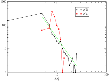
Figure 2: The degree distribution of $p(k)$ and $p(q)$ for Escherichia coli, data taken form the BIGG database BIGG .The line indicates the power-law $p(k)=k^{-\gamma}$ with $\gamma=3.0$.

Solving the BP equations for the cavity distributions the marginal probability of a flux $s_{i}$ is given by

$$p_{i}(s_{i}) = \frac{1}{C_{i}}\prod_{\nu\in N(i)}\prod_{j\in N(\nu)\backslash i}\left[\int ds_{j}p_{j\rightarrow\nu}(s_{j})\right]$$

$$\prod_{\nu\in N(i)}\delta(\sum_{j}\xi_{j,\nu}s_{j}+\xi_{i,\nu}s_{i}-g_{\nu}).$$

The distribution of the fluxes producing/consuming the metabolite $\mu$ , i.e. $\underline{S}_{\mu}=\{s_{i}\}_{i\in N(\mu)}$ is given by

$$p_{\mu}(\underline{S}_{\mu})=\frac{1}{C_{\mu}}\delta(\sum_{j}\xi_{j,\mu}s_{j}-g_{\mu})\prod_{j\in N(\mu)}p_{j\rightarrow\mu}(s_{j})$$ (5)

The entropy of the metabolic network can be expressed as

$$\Sigma = -\sum_{\mu}\int\prod_{i\in N(\mu)}ds_{i}p_{\mu}(\underline{S}_{\mu})\log p_{\mu}(\underline{S}_{\mu})+$$ (6)

$$\sum_{i}(k_{i}-1)\int ds_{i}p_{i}({s}_{i})\log p_{i}({s}_{i}).$$

The optimized state of a random metabolic network- We assume that the metabolic network is a random graph with $M$ metabolites with degree distribution $p(k)$ and $N$ reaction nodes with degree distribution $p(q)$. In this network the total number of links is given by $N\langle{q}\rangle=M\langle{k}\rangle$. In Figure 2 we show an example of $p(k)$ and $p(q)$ distributions for Escherichia coli. The $p(k)$ degree distribution for this organism is power-law $p(k)\sim k^{-\gamma}$ with an exponent $\gamma\simeq 3$ while the $p(q)$ distribution is much more picked. In different organisms the distribution of $p(q)$ and $p(k)$ do change but the general scenario of power-law $p(k)$ distribution and finite scale $p(q)$ distribution remains unchanged.

To solve the BP equations $(\ref{BP})$ in this random ensemble of graphs with given $p(k)$ and $p(q)$ degrees distributions we introduce the quantity

$$P(s)=\frac{1}{\langle{q}\rangle N}\sum_{i,\mu\in\partial i}\left\langle{\overline{p_{i\rightarrow\mu}(s)}}\right\rangle_{\rho(g)}$$ (7)

where the overline $\overline{\ldots}$ indicates the average over random sign of the reactions and the outgoing and ingoing flux distribution i.e. over the distribution for the $\{\xi\}$ $P(\{\xi\})=\prod_{i}\prod_{\nu\in\partial i}\frac{1}{2}\left[\delta(\xi_{i,\nu}-1)+\delta(\xi_{i,\nu}+1)\right]$ and $\langle{\ldots}\rangle$ indicates the average over the probability distribution $\rho(g)$ of the $g$’s. In particular we take

$$\rho(g)=p_{1}\delta(g+g_{1})+p_{2}\delta(g-g_{2})+(1-p_{1}-p_{2})\delta(g)$$ (8)

where $p_{1}$ and $p_{2}$ indicate respectively the fraction of input metabolites and the fraction of metabolites in the biomass definition and where $g_{1}$ is fixed by the environment conditions and $g_{2}$ is the rate of the biomass.

The Fourier transform of $P(s)$ is the function $\chi(w)$,

$$\chi(w)=\int dse^{iws}P(s).$$ (9)

where $w=\frac{2\pi}{L}n$. The function $\chi(w)$ satisfies the self consisted equation

$$\chi(w) = \sum_{q}\frac{qp(q)}{\langle{q}\rangle}\prod_{\nu=1}^{q-1}\left\{\sum_{k_{\nu}}\frac{k_{\nu}p(k_{\nu})}{\langle{k}\rangle}\sum_{\{n_{\nu}\}}\sum_{\omega_{\nu}}\left[\frac{1}{2}(\chi(-\omega_{\nu})+\chi(\omega_{\nu}))\right]^{k_{\nu}-1}\right\}\left\langle{\frac{e^{-i\sum_{\nu}\omega_{\nu}{g_{\nu}}}}{C(\{k_{\nu}\})}}\right\rangle_{\rho(g)}\delta(\sum_{\nu}\omega_{\nu}(-1)^{n_{\nu}}-w).$$

where $\langle{\cdot}\rangle$ indicates the average over the distribution of the incoming/outgoing fluxes $g$ and where and we have assumed $L\gg 1$ allowing for a continuous variables $\omega_{\nu}$, $w$.

$$C(\{k_{\nu}\}) \simeq \prod_{\nu=1}^{q-1}\left\{\sum_{\omega_{\nu}}\left[\frac{1}{2}(\chi(-\omega_{\nu})+\chi(\omega_{\nu}))\right]^{k_{\nu}-1}\right\}$$ (10)

$$e^{-i\sum_{\nu}{\omega_{\nu}}g_{\nu}}\delta(\sum_{\nu}\omega_{\nu}(-1)^{n_{\nu}}).$$

The equation for $\chi(w)$ will have solutions until the rate of biomass production ${g}_{2}<G_{c}$ with $G_{c}$ been corresponding to the maximal allowed biomass production of the metabolic network.

Close to the critical point ${g}_{2}\simeq G_{c}$ we suppose that the distribution $P(s)$ will scales as

$$P(s)=s^{-\tau}\Phi(s|{g}_{2}-G_{c}|^{\sigma})$$ (11)

where $\Phi$ is a scaling function. In the limit of large $L$ we can assume that $w$ (together with the $\omega_{\nu}$) is a continuous variable and we can do an asymptotic expansion is reflected the scaling behavior of $\chi(w)$, i.e.

$$\chi(w)=1-|w|^{\tau-1}h(w/|{g}_{2}-G_{c}|^{\sigma}).$$ (12)

Solving then the self consistent equation for $\chi(w)$ Eq. $(\ref{sf})$ for analytic distribution $p(q)$ and the distribution of the metabolites connectivity decaying like a power-law $p(k)\sim k^{-\gamma}$. Close to the phase transition we have

$$C(\{k_{\nu}\}) \simeq \int\dots\int\prod_{\nu=1}^{q-1}d\omega_{\nu}\left[1-(k_{\nu}-1)|\omega_{\nu}|^{\tau-1}\mbox{Re}\ h+\frac{1}{2}(k_{\nu}-1)(k_{\nu}-2)|\omega_{\nu}|^{2(\tau-1)}(\mbox{Re}\ h)^{2}\right]$$ (13)

$$e^{-i\sum_{\nu}{\omega_{\nu}}g_{\nu}}\delta(\sum_{\nu}\omega_{\nu}(-1)^{n_{\nu}})$$

$$\simeq 1+\sum_{\nu,\nu^{\prime}}\left[A_{1}(g_{\nu},g_{\nu^{\prime}})(k_{\nu}-1)(k_{\nu^{\prime}}-1)+A_{2}(g_{\nu},g_{\nu^{\prime}})(k_{\nu}-1)(k_{\nu}-2)(k_{\nu^{\prime}}-1)\right]$$

$$-\sum_{\nu,nu^{\prime},\nu^{\prime\prime}}A_{3}(g_{\nu},g_{\nu^{\prime}},g_{\nu^{\prime\prime}})(k_{\nu}-1)(k_{\nu^{\prime}}-1)(k_{\nu^{\prime\prime}}-1)$$

where $A_{1}$, $A_{2}$ and $A_{3}$ are linear functions of $g_{\nu}$, $g_{\nu^{\prime}}$ and $g_{\nu^{\prime\prime}}$. If we develop (Flux distribution of metabolic networks close to optimal biomass production) around the point $w=0$, we get

$$\chi(w) = \sum_{q}\frac{qp(q)}{\langle{q}\rangle}\prod_{\nu=1}^{q-1}\left\{\sum_{k_{\nu}}\frac{k_{\nu}p(k_{\nu})}{\langle{k}\rangle}\sum_{\{n_{\nu}\}}\int d\omega_{\nu}\left[1-(k_{\nu}-1)|\omega_{\nu}|^{\tau-1}(\mbox{Re}\ h)+\frac{1}{2}k_{\nu}(k_{\nu}-1)|\omega_{\nu}|^{2(\tau-1)}(\mbox{Re}\ h)^{2}\right]\right\}$$ (14)

$$\times\left\langle{\frac{(1-i\sum_{\nu}\omega_{\nu}{g_{\nu}})}{C(\{k_{\nu}\})}}\right\rangle_{\rho(g)}\delta(\sum_{\nu}\omega_{\nu}(-1)^{n_{\nu}}-w).$$

Since the sum over the connectivity $k_{\nu}$ are convergent in a sparse network, all metabolic networks have for the flux distribution the mean field exponents $\tau=3/2$ and $\sigma=2$ as long as the hypothesis of Flux-Balance-Analysis are satisfied.

The entropy goes like

$$\Sigma=|g_{2}-G_{c}|^{\alpha}$$ (15)

with $\alpha=\sigma(\tau-1)=1$

Therefore in the physical range for each degree distribution $p(q)$ or $p(k_{\nu})$ metabolic the predicted power-law critical exponent for the flux distribution is $\tau=3/2$ in good agreement with the Flux-Balance calculations Almaas

Conclusion- We have presented a statistical mechanics approach to study the steady state distribution of the fluxes in the metabolic network assuming optimization of the biomass. The analytic treatment finds a distribution of the fluxes which is a power-law with an mean-field exponent $\tau=3/2$ independent on the structure of the metabolic network. The method can be generalized to other critical phenomena defined on continuous variables on a finite interval, and work in this direction is in progress.
We acknowledge interesting discussions with Riccardo Zecchina, this work was supported by IST STREP GENNETEC contract No.034952.

References

- (1) S. N. Dorogovtsev, A. V. Goltsev and J. F. F. Mendes, arXiv:0705.0010 (2007).
- (2) R. Albert and A.-L. Barabási, Rev. Mod. Phys. 74, 47 (2002).
- (3) S. N. Dorogovtsev nad J. F. F. Mendes, Adv. Phys. 51, 1079 (2002).
- (4) M. E J. Newman, SIAM Review 45, 167 (2003).
- (5) R. Pastor Satorras and V. Vespignani, Evolution and Strucuture of the Internet: A statistical Physics Approach (Cambridge University Cambridge, 2004).
- (6) S. Boccaletti et al. Physics Reports 424,175 (2006).
- (7) G. Caldarelli, Scale -Free Networks (Oxford Unioversity Press, Oxford, 2007).
- (8) S. N. Dorogovtsev, A. V. Goltsev and J. F. F. Mendes, Phys. Rev. E 66, 016104 (2002).
- (9) M. Leone, V. Vázquez, A. Vepsignani and R. Zecchina, Eur. Phys. J B 28, 191 (2002)
- (10) G. Bianconi, Phys. Lett. A 303, 166 (2002).
- (11) R. Pastor-Satorras and A. Vespignani, Phys. Rev. Lett. 65, 035108 (2002).
- (12) T. Nishikawa, A. E. Motter, Y.-C. Lai and F. C. Hoppensteadt, Phys. Rev. Lett. 91, 014101 (2003).
- (13) R. Sharan and T. Ideker, Nature Biotechnology 24, 427-433 (2006).
- (14) A.L. Barabasi and Z.N. Oltvai, Nature Genetics 5, 111-113 (2004).
- (15) H. Jeong, B. Tombor, R. Albert, Z. N. Oltvai, and A.-L. Barabasi, Nature 407, 651-654 (2000).
- (16) The BIGG database can be found at the webpage http://bigg.ucsd.edu/
- (17) J. S. Edwards and B. O. Palsson, PNAS 97 5528 (2000).
- (18) E. Ravasz, A. L. Somera, D.A. Mongru, Z. N. Oltvai and A.-L. Barabási, Science 297 1551 (2002).
- (19) R. Tanaka, Phys. Rev. Lett. 94 168101 (2005).
- (20) J. S., Edwards, R. U. Ibarra and B. O. Palsson, Nature Biotechnol. 19, 125-130 (2001).
- (21) D. Segre D. Vitkup and G. M. Church, PNAS 99 15112 (2002).
- (22) T. Shlomi, O. Berkman, E. Ruppin, PNAS 102, 7695 (2005).
- (23) M. Emmerling et al., J. Bacteriol. 184,152 (2002).
- (24) E. Almaas, B. Kovacs, T. Vicsek, Z.N. Oltvai and A.-L. Barabási, Nature 427, 839-843 (2004).
- (25) J. Yedida, W. T. Freeman and Y. Weiss, in Exploring Artificial Intelligence in the New Millenniumeds. G. Lakemeyer and B. Nebel pag. 239 (2001).
- (26) A. De Martino, C. Martelli, R. Monasson and I. P. del Castillo, JSTAT P01006 (2007).
- (27) G. Bianconi and R. Zecchina, Networks and Heterogeneous Media (in press).
- (28) A. Braunstein, R. Mulet and A. Pagnani, arXiv:0709.0922 (2007).