Static Properties of Small Josephson Tunnel Junctions in a Transverse Magnetic Field

Abstract

The magnetic field distribution in the barrier of small planar Josephson tunnel junctions is numerically simulated in the case when an external magnetic field is applied perpendicular to the barrier plane. The simulations allow for heuristic analytical solutions for the Josephson static phase profile from which the dependence of the maximum Josephson current on the applied field amplitude is derived. The most common geometrical configurations are considered and, when possible, the theoretical findings are compared with the experimental data.

I Introduction

The static (and dynamic) properties of a planar Josephson Tunnel Junction (JTJ) are well understood when an external magnetic field is uniformly applied in the junction plane barone . On the contrary, very little is known when a uniform magnetic field is applied perpendicularly to the barrier plane. The main reason why, since the discovery of the Josephson effect in 1962, only few papers have dealt with a transverse magnetic fieldrc hf miller , is due to the fact that demagnetization effects imposed by the electrodes geometry are awkward to take into account. In a recent paper mon we provided an experimental proof that a transverse magnetic field can be much more capable than an in-plane one to modulate the critical current $I_{c}$ of a planar JTJ with proper barrier and electrodes geometry requirements. It is also possible to design the JTJ electrode geometry in such a way that it is totally insensitive to a transverse field. The possibility to have on the same chip JTJs having different sensitivities to an externally applied field can be very attractive in practical applications.

In this paper we push our analysis further by resorting to numerical magnetostatic simulations to find the field distribution ${\bf H}$ in the barrier plane of those JTJs having the most common rectangular and annular geometries. Once ${\bf H}$ is found empirically, the Josephson phase $\phi$, which is the difference between the complex wavefunction phases in the electrodes, can be obtained from the Josephson equationjoseph :

$${\bf\nabla}\phi=\frac{2\pi d_{e}\mu_{0}}{\Phi_{0}}{\bf H}\times{\bf n},$$ (1)

where ${\bf n}$ is a unit vector normal to the insulating barrier separating the two superconducting electrodes, $\mu_{0}$ is the vacuum permeability and $\Phi_{0}=h/2e$ is the magnetic flux quantum. If the two superconducting films have thicknesses $d_{1,2}$ and London penetration depths $\lambda_{L1,2}$ and $t_{j}$ is the barrier thickness, then the effective magnetic penetration $d_{e}$ is given bywei :

$$d_{e}=t_{j}+\lambda_{L1}\tanh{d_{1}\over 2\lambda_{L1}}+\lambda_{L2}\tanh{d_{2}\over 2\lambda_{L2}},$$

which, in the case of thick superconducting films ($d_{i}>>\lambda_{Li}$), reduces to $d_{e}\approx\lambda_{L1}+\lambda_{L2}$ (being always $d_{i}>>t_{j}$).

In Cartesian coordinates, assuming that the tunnel barrier lies in the $x-y$ plan, Eq.1 reduces to:

$$\frac{\partial\phi(x,y)}{\partial x}\propto-H_{y},\,\,\,\,\frac{\partial\phi(x,y)}{\partial y}\propto H_{x}.$$ (2)

For a planar JTJ with a uniform Josephson current density $J_{c}$ whose dimensions are smaller than the Josephson penetration depth $\lambda_{J}=\sqrt{\hbar/2e\mu_{0}d_{e}J_{c}}$, the self-induced field associated with the bias current can be neglected and the Josephson phase must satisfy the two-dimensional Laplacian equation joseph :

$$\frac{\partial^{2}\phi}{\partial x^{2}}+\frac{\partial^{2}\phi}{\partial y^{2}}=0,$$ (3)

with proper boundary conditions related to the value of the magnetic field components $H_{x}$ and $H_{y}$ on the junction perimeter. It was first pointed out in 1975hf that in a transverse applied field $\bf{H}=\rm{H_{\bot}}\bf{\hat{z}}$, the in-plane components $H_{x}$ and $H_{y}$ are ascribed to surface demagnetizing currents $\bf{j_{s}}=\bf{\hat{z}}\times\bf{H}$ feeding the interior of the junction. Since these currents mainly flow on the film edges, the largest sensitivity to a transverse field occurs when the junction is formed at the film edges. On the contrary, if the barrier is placed well inside the superconducting films, the effect of a transverse field vanishes. Our task consists of numerically evaluating the field line distribution in the barrier plane, from which we determine an empirical analytical expression $\phi(x,y)$ for the phase profile which satisfies Eq.3. Such a phase profile will allow the computation of the transverse magnetic diffraction pattern $I_{c}(H_{\bot})$ for small JTJs having different geometries and to compare it with experimental data, if available. This is achieved by recalling that the maximum Josephson current is:

$$I_{c}=I_{0}\sqrt{\langle\sin\phi\rangle^{2}+\langle\cos\phi\rangle^{2}},$$

in which the brackets $\langle\rangle$ denote spatial averages over the junction area. Throughout the paper we assume that the applied transverse field is everywhere much smaller than the critical field which would force the films into the intermediate or normal state, i.e., that the superconductors are always in the flux-free Meissner regime.

II Magnetostatic simulations

In general, magnetostatic problems are based on the magnetic vector potential. However, where no electrical currents are present, the problem can be conveniently solved using the scalar magnetic potential. In fact, in a current free region $\nabla\times\bf{H}=0$ allows the introduction of a scalar potential $V_{m}$ such that $\bf{H}=-\bf{\nabla}\rm{V_{m}}$. Using the constitutive relation $\bf{B}=\mu_{0}\mu_{r}\bf{H}$, we can rewrite Maxwell’s equation $\bf{\nabla}\cdot\bf{B}=0$ in terms of $V_{m}$:

$$-\bf{\nabla}\cdot(\mu_{0}\mu_{r}\bf{\nabla}V_{m})=0,$$ (4)

in which the magnetic relative permittivity $\mu_{r}$ is spatially dependent. We assumed that the superconducting electrodes are thicker than their London penetration depths ($d_{i}>>\lambda_{Li}$), so that the London equation reduces to $\bf{B}=0$ everywhere inside the superconductors, i.e., $\mu_{r}=0$ (perfect diamagnetism) and the normal component of the magnetic flux density vanishes at the boundary ($\bf{n}\cdot\bf{B}=0$). In the opposite limit, the films would become transparent to the transverse field and, in turn, the junction would lose its sensitivity to the transverse field. A uniform applied magnetic field $\bf{H}=\rm{H_{\bot}}\bf{\hat{z}}$ is taken into account by imposing that sufficiently far away from the junction is $V_{m}=-H_{\bot}z$. All the simulations presented in this paper were carried out setting $H_{\bot}=1A/m$.

As a consequence of the definitions of Eq.2, it is straightforward to show that Eq.3 requires that $\partial^{2}V_{m}/\partial x\partial y=\partial^{2}V_{m}/\partial y\partial x$. Further, more importantly, we have:

$$\phi(x,y)\propto\int dx\frac{\partial V_{m}}{\partial y}=-\int dy\frac{\partial V_{m}}{\partial x}.$$ (5)

The numerical solution of Eq.4 was implemented in the COMSOL Multiphysics 3D Electromagnetics module for JTJs having different rectangular and annular geometries. Models with large geometric scale variations are always problematic to mesh, in particular if they contain thin layers with large aspect ratio. Therefore, one caveat of our modeling is that, in order to keep the number of mesh elements within the PC memory handling capability, the separation between the superconducting films, i.e. the tunnel barrier thickness $t_{j}$, could not be set to realistic values for a Josephson tunnel barrier $O(1nm)$. Our numerical modeling was tested against the magnetic field distribution around a superconducting disk (with radius $R$ larger than its thickness $d$) in the plane $z=0$, centered on the $z$ axis and immersed in a field $\bf{H}=\rm{H_{\bot}}\bf{\hat{z}}$. More precisely, the radial dependence of the tangential field $H_{t}$ on the disk surface followed to a high accuracy the well known expressionlandau $H_{t}(r)\propto H_{\bot}r/\sqrt{R^{2}-r^{2}}$ everywhere except at the disk border, where the inverse square root singularity was replaced by a finite value $\hat{H}$ proportional to the square root of the disk aspect ratio $\hat{H}=H_{\bot}\sqrt{R/d}$benk . This example is indicative of the fact that, in general, the magnetostatic response of any superconducting film structure is markedly dependent on the film aspect ratio.

Figure 1: Sketch of a overlap geometry junction . The center of the junction coincides with origin of our coordinate system.

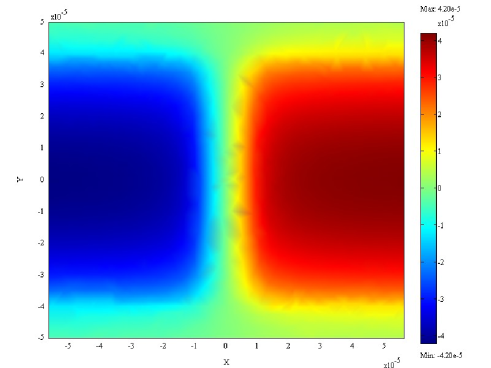
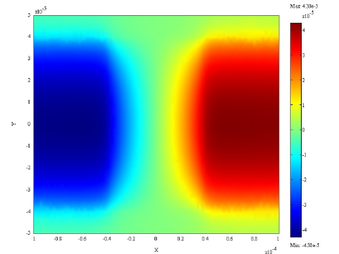
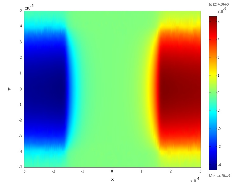
Figure 2: (Color online) Numerically obtained magnetic scalar potential $V_{m}$ (in $A$) for three overlap planar Josephson tunnel junctions having the same width $2W=80\mu m$, but different lengths: a) $2L=20\mu m$ ($\beta=0.25$), b) $2L=80\mu m$ ($\beta=1$), and c) $2L=320\mu m$ ($\beta=4$). The external applied field is $H_{\bot}=1A/m$.

III Rectangular junctions

III.1 Overlap type junctions

We begin our analysis with a JTJ obtained by the superposition of the extremities of two long and narrow parallel superconducting electrodes with equal widths. This so-called overlap geometry is depicted in Fig.1 for a square junction, i.e. $W=L$. The tunnel barrier lies in the $z=0$ plane and its center coincides with the axis origin. Further, it has a length $2L$ along the x-direction and a width $2W$ along the y-direction. In the simulations the electrodes have a thickness $d=10\mu m$ and are $t_{j}=1\mu m$ apart. The film width $2W$ and the overlapping length $2L$ where varied in order to treat barriers with different aspect ratios $\beta=L/W$. Figs.2a-c show the numerically obtained $V_{m}$ solutions in the barrier area of three overlap junctions having the same width $2W=80\mu m$, but different lengths $2L=20$, $80$, and $320\mu m$. By analyzing the properties of such plots we aim to infer an empirical, physically acceptable analytical form for $V_{m}(x,y,z=0)$. We observe that, for any value of $\beta$, the scalar potential in the barrier is symmetric with respect to the x-axis and antisymmetric with respect to the y-axis. In other words, the expression $V_{m}(x,y)$ we are looking for has to be an odd function of $x$ and a even function of $y$. Furthermore, we note that the potential decays from the junction corners over a distance $W$, being mostly null when $L>W$ (or $\beta>1$). We have checked that the following ansatz:

$$V_{m}(\hat{x},\hat{y})=W\hat{H}\cos q\hat{y}\frac{\sinh q\beta\hat{x}}{\sinh\beta},$$ (6)

in which $q$ is a fitting parameter near unity, allowed us to reproduces the plots of Figs.2a-c at a better than qualitative level. In fact, for $q=1$ the relative difference between the simulation output and the proposed expression being everywhere less than $\pm 15\%$ and the $q$ value that minimized the error was $q\simeq 0.9$. We have introduced the normalized units $\hat{x}=x/L$ and $\hat{y}=y/W$ (note that $\beta\hat{x}=x/W$). In the last equation, again $\hat{H}\propto H_{\bot}\sqrt{W/d}$, with a proportionality constant of order of unity which slightly increases when the barrier thickness $t_{j}$ decreases. Unfortunately, recalling the comments of the previous section, we cannot be more precise on this point.

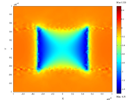
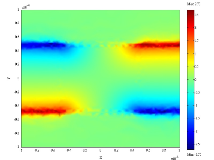
Figure 3: (Color online) Numerically obtained in-plane magnetic field components in $A/m$ for a square overlap junction having $2W=2L=100\mu m$ in a transverse externally applied field $H_{\bot}=1A/m$. Color plots for a) $H_{x}(x,y,z=0)$ and b) $H_{y}(x,y,z=0)$.

Now we focus our attention on the components of the magnetic field in the barrier plane $H_{x}(x,y)=-\partial V_{m}/\partial x|_{z=0}$ and $H_{y}(x,y)=-\partial V_{m}/\partial y|_{z=0}$ ($H_{z}$ being identically null all over the barrier area). They are shown in Fig.3a and b, respectively, for the particular case $W=L=100\mu m$. We like to specify, at this point, that the same plots obtained from numerical simulations based on the vector, rather than scalar, potential differed by no more than $\pm 10\%$, the discrepancy being larger at the barrier edges. From Eq.6 with $q=1$, the following analytical expressions are derived:

$$H_{x}(\hat{x},\hat{y})=-\hat{H}\cos\hat{y}\frac{\cosh\beta\hat{x}}{\sinh\beta},$$ (7)

$$H_{y}(\hat{x},\hat{y})=\hat{H}\sin\hat{y}\frac{\sinh\beta\hat{x}}{\sinh\beta}.$$ (8)

The physical meaning of the last expressions is that for $\beta=L/W>1$, the magnetic field lines are confined to the corners of the junctions at a distance $W$ and most of the field lines entering the junction at $x=\pm L$ are bent by $90^{o}$ and leave at $y=\pm W$. In the opposite limit, $\cosh\beta x\approx 1$, so the x-dependence of $H_{x}$ disappears, meaning that all the field lines entering the barrier at, say, $x=-L$ exit at $x=L$ (or viceversa). Further, we notice that while the $x$-component is negative all over the barrier area, the $y$-component symmetrically spans from negative to positive values. Due to the linearity of Eq.4 e the system symmetry with respect to the $z=0$ plane, if the direction of the transverse field is reverted, then $H_{x}$ and $H_{y}$ simply invert their sign. The magnetic field line distributions in the junction barrier corresponding to the scalar potentials of Figs.2a-c are shown in Figs.4a-c. Similar plots based on the previous analytical expressions would be practically undistinguishable at the picture resolution level, therefore, they will not be shown. From the magnetic field distributions we expect that, for a given junction area $LxW$, the critical current $I_{c}$ of a planar JTJ with pure overlap geometry ($L<W$) modulates much faster than that of a sample with pure in-line geometry ($L>W$). At a first sight, it might seem that the effect of a transverse field is qualitatively similar to that of an in-plane field applied along the film direction, i.e. along the $x$-axis, in our case. However, this is not true at a quantitative level because, in general, $H_{x}(x,\pm W)$ is not constant in a transverse field.

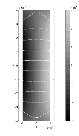
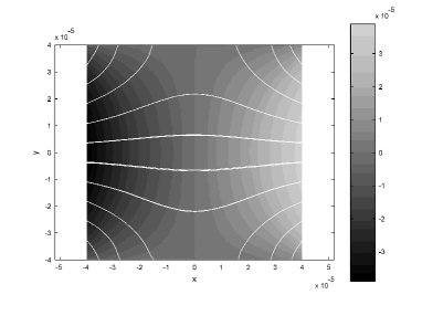
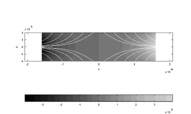
Figure 4: Magnetic field lines inside three overlap planar Josephson tunnel junctions having the same width $2W=80\mu m$, but different lengths: a) $2L=20\mu m$ ($\beta=0.25$), b) $2L=80\mu m$ ($\beta=1$) and c) $2L=320\mu m$ ($\beta=4$).

Inserting Eq.6 in any of the Eq.5, we derive an approximate analytical expression for the Josephson phase profile:

$$\phi(\hat{x},\hat{y})=h\sin\hat{y}\frac{\cosh\beta\hat{x}}{\sinh\beta},$$ (9)

where $h=2\pi d_{e}W\mu_{0}\hat{H}/\Phi_{0}$ is a dimensionless parameter proportional to the applied transverse field amplitude $H_{\bot}$ through $\hat{H}$. It is easy to verify that the last expression, in which we have omitted an integration constant $\phi_{0}$, satisfies Eq.3.

With $\phi$ an odd function of $\hat{y}$, then $\langle\sin\phi\rangle=0$; therefore, the magnetic pattern $I_{c}(h)$ reduces to:

$$I_{c}(h)=I_{c}(0)\int_{0}^{1}d\hat{x}\int_{0}^{1}d\hat{y}\cos\phi(x,y).$$ (10)

Fig.5a-c show the computed transverse magnetic patterns for the three values of the barrier aspect ratio $\beta$ used before ($4$, $1$ and $0.25$). As expected the response to a transverse field is very weak for an in-line JTJ, the first minimum occurring at $h\simeq 74$ for $\beta=4$. The secondary pattern maxima become more pronounced for a pure overlap geometry. However, in the limit $L<<W$, all the above equations lose their validity when the overlapping length becomes comparable with the film thickness.

Figure 5: Computed transverse magnetic patterns $I_{c}(h)$ for an overlap junction with different $L/W$ ratios: a) inline junction $L=4W$, b) square overlap $L=W$ and c) pure overlap junction $W=4L$.

It is important to stress here that we are dealing with electrically small JTJs, therefore the different shapes of the transverse magnetic pattern is a direct consequence of the different distribution of the surface screening currents (and not of the applied bias current). Unfortunately, there are no data available in the literature to check the validity of our theoretical magnetic diffraction patterns for a small overlap JTJ formed by films having the same widths. In fact, the experiments reported by Rosestein and Chen in 1975rc refer to an overlap JTJ formed by two thick $Pb$ electrodes of unequal widths ($2W=0.74mm$ and $2W^{\prime}=1.00mm$) and a common overlay region of $2L=0.35mm$. It is quite evident that, for such geometrical film configuration, the symmetry with respect to the $y$-axis is broken and Eq.9 is unable to correctly describe the magnetic field (and screening currents) distribution. Fig.6a and b show, respectively, the result of numerical simulations carried out for the specific electrode configuration of Ref.rc and the corresponding $I_{c}(h)$. According to Ref.hf , we believe that difference between the experimental data of Ref.rc and the numerical prediction of Ref.hf valid only for the specific case $\beta=0.5$, arises from the unequal widths of the films in the experiment. Indeed, the magnetic diffraction pattern reported in Ref.hf is of a piece with the curve in Fig.6b.

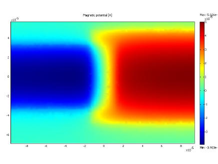
Figure 6: (Color online) a) Numerically obtained scalar potential for an overlap junction obtained by the superposition of two films of unequal widths $2W=0.74mm$ and $2W^{\prime}=1.00mm$. The overlapping distance is $2L=0.35mm$, as for the sample quoted in Ref.rc . b)Computed magnetic pattern $I_{c}(h)$ for an overlap junction with aspect ratio $L/W=0.5$.

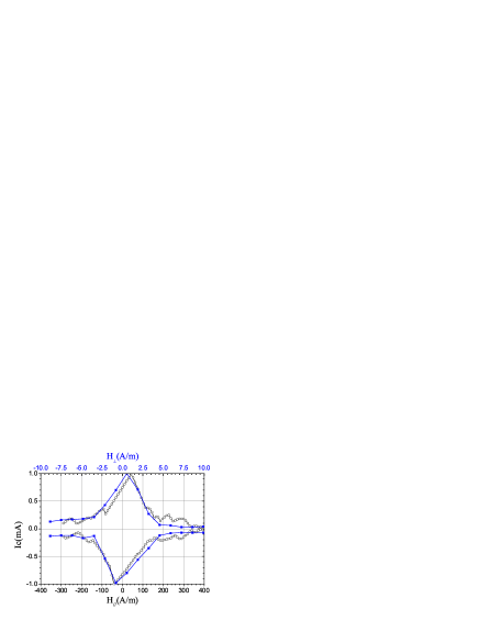
Figure 7: a) (Color online) Comparison between the diffraction patterns measured in a parallel (black bottom axis) and transverse (blue top axis) field of a $Nb/Al_{ox}/Nb$ overlap-type junction with $\lambda_{J}\sim 50\mu m$ whose length is $500\mu m$, while the width is equal to $4\mu m$. b)Geometry details: the base (red) and top (blue) electrode widths are $540$ and $506\mu m$, respectively. The barrier area is delimited by the black rectangle.

We conclude this section considering that, for unidimensional overlap junctions for which $W>\lambda_{j}>L$, being $\frac{\partial^{2}\phi}{\partial x^{2}}<<\frac{\partial^{2}\phi}{\partial y^{2}}$, then the Josephson phase has to obey to the equation first introduced by Owen and Sacalapinoowen :

$$\frac{d^{2}\phi}{dy^{2}}=\frac{1}{\lambda_{j}^{2}}sin\phi$$ (11)

when an in-plane external field is applied along the x-direction. In fact, Fig.7a shows the comparison between the diffraction patterns measured in a parallel and transverse field of a $Nb/Al_{ox}/Nb$ overlap-type junction with $\lambda_{J}\sim 50\mu m$ whose length is $500\mu m$, while the width is equal to $4\mu m$. The base and top electrode widths are $540$ and $506\mu m$, respectively. The junction geometry is depicted in Fig.7b. We observe that the two experimental datasets almost overlap, when a factor scale of about $40$ is applied on the abscissae, meaning that the sample is much more sensitive to a transverse field rather than an in-plane one.

III.2 Cross type junctions

Figure 8: Sketch of a square cross type junction. The center of the junction coincides with the axis origin.

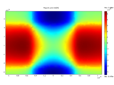
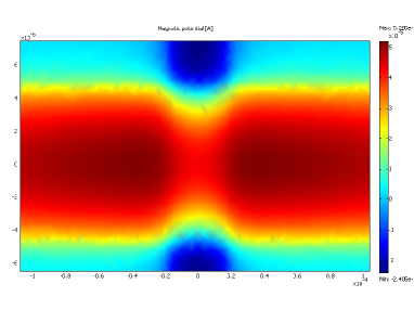
Figure 9: (Color online) Numerically obtained magnetic scalar potential $V_{m}$ (in $A$) in the barrier plane for three cross type junctions having the same width $2W=100\mu m$, but different lengths: a) $2L=100\mu m$ ($\beta=1$), b) $2L=40\mu m$ ($\beta=0.4$), and c) $2L=20\mu m$ ($\beta=0.2$). The external applied field is $H_{\bot}=1A/m$.

Cross geometry JTJs are formed by the superposition of two perpendicular superconducting electrodes, as depicted in Fig.8. The static properties of such junctions in a transverse magnetic field were analyzed by Miller et al.miller , but only in the particular case of equal film widths $2L=2W$. They proposed, as an approximate solution of Eq.3, a phase profile $\phi(x,y)\propto xy$ (corresponding to a saddle shaped scalar magnetic potential $V_{m}(x,y)\propto x^{2}-y^{2}$ and to a monotonically decreasing $I_{c}(H_{\bot})$.) We want to generalized these results for junctions with non unitary aspect ratios $\beta=L/W$. Figs.9a-c display the numerical solutions of Eq.4 for three cross junctions having the same width $2W=100\mu m$, but different lengths $2L=100$, $40$, and $20\mu m$. We observe that, for any value of $\beta$, the scalar potential in the barrier is four-fold symmetric meaning that the empirical expression $V_{m}(x,y)$ we are looking for has to be an a even function of both $x$ and $y$. Further, $V_{m}$ always vanishes at the junction corners and, as the junction length shrinks, the scalar potential distribution gets more and more uniform over the barrier area. A careful analysis of the scalar potential plots in Figs.9a-c, led us to the following expression:

$$V_{m}(\hat{x},\hat{y})=\hat{H}\sqrt{WL}\left(\cos q\hat{y}\frac{\cosh q\beta\hat{x}}{\cosh\beta}-\cos q\hat{x}\frac{\cosh q\hat{y}/\beta}{\cosh 1/\beta}\right),$$ (12)

in terms of normalized variables. Here again $q$ is a fitting that can be comfortably set equal to unity. More specifically, with $q=1$, the relative difference between the simulation output and the heuristic expression of Eq.12 was numerically found to be everywhere less than $\pm 15\%$ although it was minimized by $q\simeq 1.2$. The proposed expression is made up by two terms which can be seen as the contributions from the two electrodes. When $L=W$, the two terms have the same weights ($\textrm{sech}1\simeq 0.65$), but, for, say, $\beta<1$, the weight of the first term is larger than the one of the second term and viceversa. Further, in the limit $\beta<<1$ the first weight saturates to unity while the second vanishes.

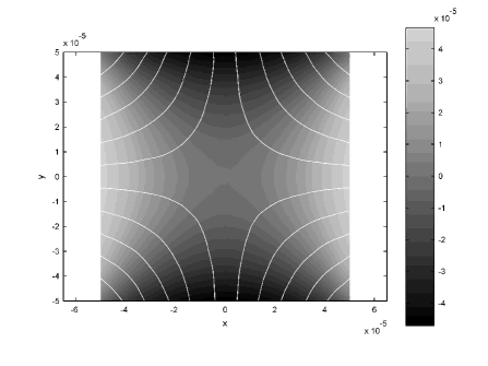
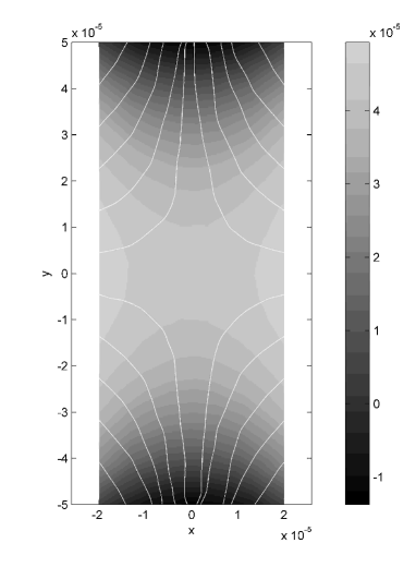
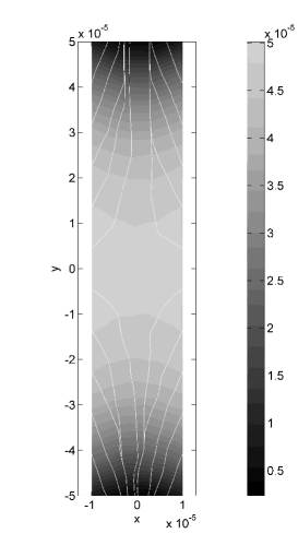
Figure 10: Numerically obtained magnetic field distribution in the barrier area of three cross-type planar Josephson tunnel junctions having the same width $2W=100\mu m$, but different lengths: a) $2L=100\mu m$ ($\beta=1$), b) $2L=40\mu m$ ($\beta=0.4$) and c) $2L=20\mu m$ ($\beta=0.2$).

From Eq.12 with unitary $q$, the Josephson phase profile can be easily derived:

$$\phi(\hat{x},\hat{y})=h\left(\sin\hat{y}\frac{\sinh\beta\hat{x}}{\cosh\beta}+\sin\hat{x}\frac{\sinh\hat{y}/\beta}{\cosh 1/\beta}\right),$$ (13)

where $h=2\pi d_{e}\sqrt{WL}\mu_{0}\hat{H}/\Phi_{0}$ and with Eq.3 being identically satisfied. We begin with the observation that setting $\beta=1$ and retaining the first two terms in the Taylor expansion of the trigonometric and hyperbolic functions, Eqs.13 and 12 reduces to $\phi(x,y)\propto xy-x^{3}y^{3}/36$ and $V_{m}(x,y)\propto x^{2}-y^{2}$, as it should be. Further, upon the inversion of $\beta$, $\phi(\hat{x},\hat{y})=\phi(\hat{y},\hat{x})$, meaning that the solutions for two junctions having reciprocal aspect ratios differ by a rotation of $\pm 90^{o}$. Figs.10a-c show the magnetic field distributions in the barrier area corresponding to the scalar potentials shown in Figs.9a-c.

Again, with $\langle\sin\phi\rangle=0$, the magnetic diffraction pattern for a cross junction in a transverse magnetic field are found on inserting the expression above in Eq.10. Fig.11 shows $I_{c}(h)$ for the three values of the barrier aspect ratios considered in Figs.9a-c, i.e., $\beta=1$, $0.4$, and $0.2$. For the considerations above, the red and black curves in Fig.11 also represent the $I_{c}(h)$ for $\beta=2.5$ and $5$, respectively. We come to the interesting result that for cross junctions in a transverse field the critical current decreases monotonically with the field amplitude $H_{\bot}$ and, for large fields ($h>>1$), $I_{c}(h)\propto 1/H_{\bot}$ (see the log-log plot in the inset of Fig.11). The experimental transverse pattern presented in Ref.miller bears strong resemblance to the $I_{c}(h)$ obtained for $\beta=1$.

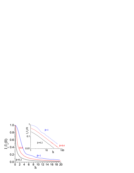
Figure 11: (Color online) Computed transverse magnetic patterns $I_{c}(h)$ for a cross junction with different $L/W$ ratios $\beta=1$, $\beta=0.4$ and $\beta=0.2$. In the inset the log-log plot shows that for large fields $I_{c}(h)\propto 1/h$.

IV Annular junctions

In this section we will examine the behavior of small annular JTJs in the presence of a transverse magnetic field. Denoting the inner and outer ring radii, respectively, as $r_{i}$ and $r_{o}$, we assume that the annular junction is unidimensional, i.e., the ring mean radius $\overline{r}=(r_{i}+r_{o})/2$ is much larger than the ring width $\triangle r=(r_{o}-r_{i})/2$.

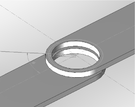
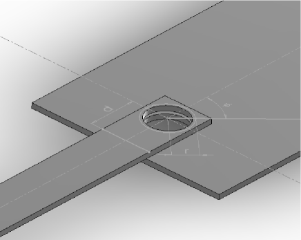
Figure 12: (Color online) Sketches of the two types of annular JTJs considered in this paper. a) Lyngby type geometry made by two films whose widths match the ring diameter. b) Asymmetric annular junctions made by two films with unequal widths.

Using polar coordinates, the Josephson equation Eq.1 can be split into:

$${{\partial\phi}\over{\partial r}}=\kappa H_{\theta}\quad,\,\,\,\,\quad{{\partial\phi}\over{r\partial\theta}}=-\kappa H_{r},$$ (14)

where $H_{r}$ and $H_{\theta}$ are the radial and tangential components of the magnetic field in the ring plane, respectively and $\kappa$ depends on the electrodes geometrical configurationprb96 . With the annulus unidimensional, we can neglect the radial dependence of the Josephson phase $\phi(r,\theta)=\phi(\overline{r},\theta)$ and, henceforth:

$$\phi=\phi(\theta)=-\kappa\overline{r}\int d\theta H_{r}(\overline{r},\theta)+const.$$ (15)

In the well known case of a spatially homogeneous in-plane field $\bf{H_{\|}}$ applied in the direction of $\theta=0$, then $H_{r}=H_{\|}\ \cos\theta$ (and $H_{r}=H_{\|}\ \sin\theta$), so that the last integral yieldsbr96 :

$$\phi(\theta)=h\sin\theta+\phi_{0},$$ (16)

where $h\propto H_{\|}$ and $\phi_{0}$ is an integration constant. Assuming that the Josephson current density $J_{c}$ is constant over the ring circumference, the Josephson current through the barrier is obtained by:

$$I_{c}(h)=\frac{I_{c}(0)}{2\pi}\int_{-\pi}^{\pi}d\theta\sin\phi(\theta).$$

in which $I(0)=J_{c}2\pi{\bar{r}}\Delta r$ is the maximum junction critical current which occurs in zero field. As far as $\phi(\theta)$ is an odd function (when $\phi_{0}=0$), the calculation of the maximum critical current reduces to the following integration:

$$I_{c}(h)=\frac{I_{c}(0)}{\pi}\int_{0}^{\pi}d\theta\cos\phi(\theta).$$ (17)

Inserting $\phi$ given by Eq.16, we obtain for the maximum critical currentprb96 ,

$$I_{c}(h)=I_{c}(0)\bigl{|}J_{0}(h)\bigr{|},$$ (18)

in which $J_{0}$ is the zero order Bessel function (of first kind). The periodic conditions for the phase difference $\phi$ and its angular derivative around an annular junction are:

$$\phi(\theta+2\pi)=\phi(\theta)+2\pi n,$$ (19)

$${{d\phi(\theta+2\pi)}\over{d\theta}}={{d\phi(\theta)}\over{d\theta}},$$ (20)

where $n$ is an integer corresponding to the net number of fluxons (i.e., number of fluxons minus number of antifluxons) trapped in the junction at the time of the normal-to-superconducting transition. Eqs.(19) and (20) state that observable quantities such as the Josephson current (through $\sin\phi$) and the radial magnetic field (through $d\phi/d\theta$) must be single valued upon a round trip; they were derived in Ref.prb96 starting from the fluxoid quantization.

Eq.16 and Eq.18 hold under the assumption that there are no fluxons trapped in the barrier; however, they can be easily generalized to the case of $n\neq 0$ trapped fluxons. In such case, Eq.16 changes to:

$$\phi(\theta)=h\sin\theta+n\theta+\phi_{0},$$ (21)

in which the linear term in Eq.21 takes into account the phase twist due to the presence of the trapped fluxons, being that the ring circumference is smaller or comparable to the fluxon rest length. Carrying out the integration in Eq.17 with $\phi$ given by Eq.21 and maximizing with respect to $\phi_{0}$, we get:

$$I_{c}^{n}(h)=I_{c}(0)\bigl{|}J_{n}(h)\bigr{|},$$ (22)

in which $J_{n}$ is the n-th order Bessel function. Eqs.18 and 22 have been experimentally verified in a number of papers.

A Lyngby type annular JTJ, firstly reported in 1985 by Davidson et al.davidson , is obtained by two films having the same width, as schematically depicted in Fig.12a. Further, Fig.12b shows a different kind of annular JTJ for which the film widths are quite different: we will call it asymmetric annular junction. At the end of this section we will present experimental data for such asymmetric geometrical configuration. We have carried out magnetostatic simulation for the two annular geometries depicted in Figs.12 when the applied field is transverse. Only the case of no trapped fluxons was considered, corresponding to zero net magnetic flux through the superconducting holes. Contrary to the case of the rectangular bidimensional JTJs considered previously, now we do not have to know the magnetic field distribution in the junction plane, but, by virtue of Eq.14b, we can limit our interest to just the angular dependence of the radial magnetic field $H_{r}(\overline{r},\theta)$. In our simulations we set $r_{i}=40\mu m$ and $r_{o}=50\mu m$, so that $\overline{r}=45\mu m$. For the asymmetric configuration the film widths were chosen to be $2W=100\mu m$ and $2W^{\prime}=200\mu m$.

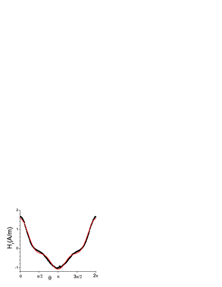
Figure 13: (Color online) Angular dependencies of the radial magnetic field $H_{r}(\theta)$ for a small annular junction in a transverse field having: a) Lyngby type geometry sketched in Fig.12a and b) asymmetric geometry sketched in Fig.12b. In the numerical simulations the amplitude of the transverse field was set to $1A/m$.

Postprocessing the simulation outputs we found out that, in the case of Lyngby geometry, $H_{r}$ follows very closely a sinusoidal dependence on $\theta$, as shown in Figs.13a: more specifically, by choosing the angle origin in such a way that $\theta=0$ corresponds to the positive x-axis direction, we have $H_{r}\propto\cos\theta$, exactly as if the magnetic field were applied in the ring plane. By integration we get Eq.21 again with $h$ depending on the geometrical film configuration and being proportional to the transverse field amplitude $H_{\bot}$. We come to the remarkable conclusion that the diffraction pattern of an electrically small annular junction with no trapped flux in a transverse field follows the zero order Bessel function behavior, as if the field were applied in the barrier plane.

The situation is quite different when we consider asymmetric annular junctions. In fact, as shown in Fig.13b, it is quite evident that now the slope of the radial field changes abruptly for $\theta\simeq\pi/2$ and $\theta\simeq 3\pi/2$ resulting in a periodic asymmetric ratchet-like potential $dH_{r}/d\theta$. We have numerically checked that to a high accuracy $\int_{0}^{2\pi}d\theta H_{r}(\theta)=0$, as it should be when no fluxons are trapped in the junction. In order to correctly reproduce $H_{r}(\theta)$, we have to consider higher $\theta$ harmonics. It was found that a truncated Fourier expansion cast in the form:

$$H_{r}(\theta)\propto\cos\theta+2\gamma\cos 2\theta+3\delta\cos 3\theta$$ (23)

can satisfactorily fit our numerical findings. The two fitting parameters $\gamma$ and $\delta$ can be ascribed to two degrees of freedom in the layout geometry: the ratio of the top and bottom film widths and the distance from the junction to the edge of the bottom film. Eq.23 with $\gamma=0.11$ and $\delta=0.085$ is shown as a solid red line in Fig.13b.

By integrating Eq.14b with $H_{r}$ given by Eq.23, we get an approximate expression for the angular phase dependence:

$$\phi(\theta)\approx h(\sin\theta+\gamma\sin 2\theta+\delta\sin 3\theta)$$ (24)

in which still $\phi(-\theta)=-\phi(\theta)$, but the symmetries $\phi(\pi/2-\theta)=\phi(\pi/2+\theta)$ and $\phi(3\pi/2-\theta)=\phi(3\pi/2+\theta)$ are now lost. Since $\phi(\theta)$ is an odd function, Eq.17 allows us to calculate the magnetic diffraction patterns corresponding to the above non-sinusoidal phase profile, even in the case when a term $n\theta$ is added to account for the presence of $n$ trapped fluxons. It turned out that, while for $n=0$ the effects of the $\gamma$ and $\delta$ terms tend to cancel each other, resulting in a zero-order Bessel function behavior as in Eq.18, for $n\neq 0$ we found a marked departure from the $n$-th order Bessel function dependence of Eq.22. These results are supported by experimental results for an asymmetric annular junction ($\overline{r}=80\mu m$ and $\Delta r=4\mu m$) made by unequal width films: the base electrode width is $540\mu m$ and the top electrode width is $170\mu m$. For such layout, the numerical analysis of the angular radial field dependence yielded the best fit values $\gamma=0.19$ and $\delta=0.078$. In the Figs.14a and b we show, respectively, the experimental diffraction patterns (dots) for such junction without trapped fluxons and with $n=1$ trapped fluxon. The experimental data can be fitted very nicely by the theoretical expectations (solid red lines) obtained inserting the above $\gamma$ and $\delta$ values in Eq.24.

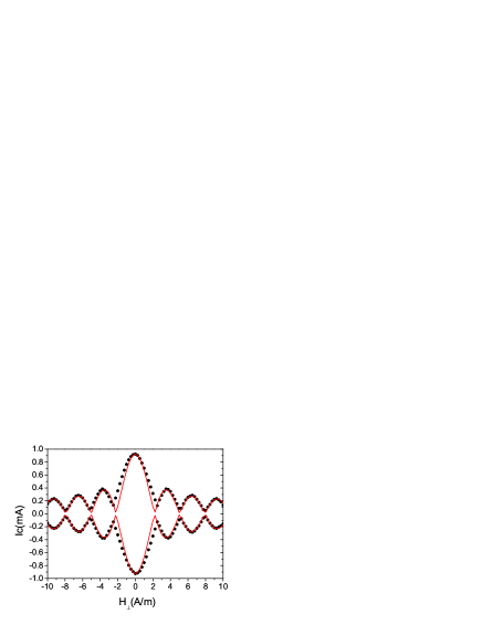
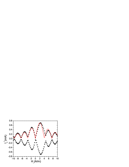
Figure 14: (Color online) Transverse diffraction patterns for an asymmetric annular junction. The dots are the experimental data, while the solid red lines are the theoretical expectations obtained inserting $\gamma=0.18$ and $\delta=0.08$ in Eq.24. a) no trapped fluxon; b) one trapped fluxon.

We observe that when no fluxons are trapped in the asymmetric annular junctions the transverse pattern is definitely symmetric with respect to the inversion of field direction and is barely distinguishable from the pure Bessel one; further, we stress that the same sample measured with an in-plane field applied in the $\theta=0$ direction showed again a Bessel like pattern, but the response to the applied field was about 25 times weaker.

On the contrary, with $n=1$ the transverse magnetic diffraction pattern loses its symmetry with respect to the field amplitude, i.e. $I_{c}^{1}(-h)\neq I_{c}^{1}(h)$. Furthermore, both in the experiments and in the calculations, it turns out that $I_{c}^{1}(-h)=I_{c}^{-1}(h)$; in other words, if we invert both the field and fluxon polarities we obtain the same magnetic diffraction pattern. This result was obtained and exploited in the context of a detailed investigation of the symmetry breaking during fast normal-to-superconducting phase transitions of annular JTJs recently publishedKZ . Among other things, it has been experimentally and theoretically demonstrated that when a small transverse field is applied to the ring during the thermal quench the probability to trap a Josephson fluxon can be very close to unity, the fluxon polarity depending on the field polarity. The ability to easily discriminate between a fluxon and an antifluxon can be conveniently exploited in the recently proposed Josephson-vortex qubits experiments with ring and heart-shaped JTJsclarke . The asymmetry of the magnetic diffraction pattern can be very simply ascribed to the ratchet-like potential whose effect on the fluxon dynamic properties has been fully investigated recentlygoldobin .

We conclude this section by remarking that the angular dependence of both the radial and tangential magnetic field components in the barrier of a annular JTJ do not change if the circular hole is removed from one of the electrodes. This is supported by both numerical simulations and experimental dataprb98 . Indeed, when the ring shaped barrier is formed between a holed film and a singly connected one, the Josephson fluxon polarity is univocally related to the polarity of the quantized flux threading the hole.

V Concluding remarks

The transverse magnetic patterns of electrically small Josephson tunnel junctions have been derived numerically by solving the magnetostatic problem for different geometrical configurations of the junction electrodes and of the barrier. More specifically, from the numerical analysis of the magnetic scalar potential produced in the barrier plane by the demagnetizing currents circulating on the electrode surfaces we derived approximate and simple expressions for the Josephson phase distribution in the barrier area, which, in turn, permitted to calculate the junction critical current. Such calculations show, among other things, that for rectangular barriers the modulation of the maximum critical current never follows the Fraunhofer behavior typical of a field applied in the barrier plane; further, $I_{c}(H_{\bot})$ strongly depends on the barrier aspect ratio $L/W$. On the contrary, the critical current modulation in a transverse field of annular JTJs without trapped fluxons is fairly close to the one corresponding to a parallel field, although it can be much faster when the field is perpendicular. When the film configuration of the annular junction is asymmetric, then the static properties depend on the polarity of the transverse field and of the trapped fluxons. It’s worthy to mention that our calculations were carried out assuming that the junctions were not biased. However, in order to measure the magnetic diffraction patterns one needs to supply a transport current by an external source. As far as the JTJ is electrically small, as in cases considered in this paper, the effect of a non uniform current distribution through the barrier is negligiblebarone . Nevertheless, to exclude flux from the electrodes interiors, a self-field that wraps around the films is generatedRose-Innes whose effect on the Josephson phase distribution is largest when the current is largest. This situation typically occurs when the applied field is small (or absent) regardless of its orientation with respect to the barrier plane. As the external field amplitude grows, the relative effect of bias induced screening currents decreases, and disappears when the field amplitude is such that the critical current is zero.

It is important to stress that the static properties of a small JTJ in a transverse field is strictly related to the film layout. In the case of junctions formed in a windows between two films which completely overlap each other near the junction itself, the circulating currents on the film interior surfaces are symmetric with respect to the barrier plane and result in a zero magnetic field; consequently such JTJs will remain totally insensitive to a transverse field: this holds for overlap type and annular geometry JTJs shown, respectively, in Fig.1 and Fig.12a when one of the electrodes is rotated by $180^{o}$. As mentioned in the Introduction, we also expect a very small sensitivity to a transverse field when the barrier window is located well inside the superconducting electrodes. The possibility to design multijunction chips whose each junction has its own magnetic diffraction pattern makes the physics and the application of transverse field very attractive and promising. Unfortunately, so far, very few experimental works have dealt with transverse field because of lack of theoretical understanding. We believe that this paper will stimulate other groups to fill the gap.

References

- (1) A. Barone and G. Paternò Physics and Applications of the Josephson Effect (Wiley, New York, 1982).
- (2) I. Rosenstein and J.T. Chen, Phys. Rev. Lett. 35 303-305 (1975).
- (3) A.F. Hebard and T.A. Fulton, Phys. Rev. Lett. 35 1310-1311 (1975).
- (4) S.L. Miller, Kevin R. Biagi, John R. Clem, and D.K. Finnemore, Phys. Rev. 31, 2684 (1985).
- (5) R. Monaco, M. Aaroe, J. Mygind, V.P. Koshelets, J. Appl. Phys.102, 093911 (2007).
- (6) B. D. Josephson, Rev. Mod. Phys. 36, 216 (1964).
- (7) M. Weihnacht, Phys. Status Solidi 32, K169 (1969).
- (8) L.D. Landau and E.M. Lifshitz, Electrodynamics of Continuous Media (Addison-Wesley, Reading, 1960).
- (9) M. Benkraouda and John R. Clem, Phys. Rev. B 53, 5716 (1996).
- (10) C.S. Owen and D.J. Scalapino, Phys. Rev. 164, 538-544 (1967).
- (11) R. Monaco, J. Mygind, M. Aaroe, R.J. Rivers and V.P. Koshelets, Phys. Rev. B 77, 054509 (2008).
- (12) N. Martucciello, and R. Monaco, Phys. Rev. B 54, 9050-9053 (1996).
- (13) N. Grønbech-Jensen, P. S. Lomdahl, M. R. Samuelsen, Phys. Lett. A 154, 14 (1991).
- (14) N. Martucciello, and R. Monaco, Phys. Rev. B53, 3471-3482 (1996).
- (15) A. Davidson, B. Dueholm, B. Kryger, and N. F. Pedersen, Phys. Rev. Lett. 55, 2059 (1985).
- (16) J. Clarke, Nature (London) 425, 133 (2003).
- (17) E. Goldobin, A. Sterck, and D. Koelle, Phys. Rev. E 63, 031111 (2001) and references therein.
- (18) N. Martucciello, J. Mygind, V.P. Koshelets, A.V. Shchukin, L.V. Filippenko and R. Monaco, Phys. Rev. B 57, 5444 (1998).
- (19) A.C. Rose-Innes and E.H. Rhoderick Introduction to Superconductivity Par.8.7 (Pergamon Press, Oxford, 1969).