CDF Collaboration333With visitors from aUniversiteit Antwerpen, B-2610 Antwerp, Belgium,
bChinese Academy of Sciences, Beijing 100864, China,
cUniversity of Bristol, Bristol BS8 1TL, United Kingdom,
dUniversity of California Irvine, Irvine, CA 92697,
eUniversity of California Santa Cruz, Santa Cruz, CA 95064,
fCornell University, Ithaca, NY 14853,
gUniversity of Cyprus, Nicosia CY-1678, Cyprus,
hUniversity College Dublin, Dublin 4, Ireland,
iUniversity of Edinburgh, Edinburgh EH9 3JZ, United Kingdom,
jUniversidad Iberoamericana, Mexico D.F., Mexico,
kUniversity of Manchester, Manchester M13 9PL, England,
lNagasaki Institute of Applied Science, Nagasaki, Japan,
mUniversity de Oviedo, E-33007 Oviedo, Spain,
nQueen Mary, University of London, London, E1 4NS, England,
oTexas Tech University, Lubbock, TX 79409,
pIFIC(CSIC-Universitat de Valencia), 46071 Valencia, Spain,
xRoyal Society of Edinburgh/Scottish Executive Support Research Fellow,
Search for Heavy, Long-Lived Neutralinos that Decay to Photons at CDF II Using Photon Timing
T. Aaltonen
Division of High Energy Physics, Department of Physics, University of Helsinki and Helsinki Institute of Physics, FIN-00014, Helsinki, Finland
J. Adelman
Enrico Fermi Institute, University of Chicago, Chicago, Illinois 60637
T. Akimoto
University of Tsukuba, Tsukuba, Ibaraki 305, Japan
M.G. Albrow
Fermi National Accelerator Laboratory, Batavia, Illinois 60510
B. Álvarez González
Instituto de Fisica de Cantabria, CSIC-University of Cantabria, 39005 Santander, Spain
S. AmeriouIstituto Nazionale di Fisica Nucleare, Sezione di Padova-Trento, uUniversity of Padova, I-35131 Padova, Italy
D. Amidei
University of Michigan, Ann Arbor, Michigan 48109
A. Anastassov
Northwestern University, Evanston, Illinois 60208
A. Annovi
Laboratori Nazionali di Frascati, Istituto Nazionale di Fisica Nucleare, I-00044 Frascati, Italy
J. Antos
Comenius University, 842 48 Bratislava, Slovakia; Institute of Experimental Physics, 040 01 Kosice, Slovakia
G. Apollinari
Fermi National Accelerator Laboratory, Batavia, Illinois 60510
A. Apresyan
Purdue University, West Lafayette, Indiana 47907
T. Arisawa
Waseda University, Tokyo 169, Japan
A. Artikov
Joint Institute for Nuclear Research, RU-141980 Dubna, Russia
W. Ashmanskas
Fermi National Accelerator Laboratory, Batavia, Illinois 60510
A. Attal
Institut de Fisica d’Altes Energies, Universitat Autonoma de Barcelona, E-08193, Bellaterra (Barcelona), Spain
A. Aurisano
Texas A&M University, College Station, Texas 77843
F. Azfar
University of Oxford, Oxford OX1 3RH, United Kingdom
P. AzzurrisIstituto Nazionale di Fisica Nucleare Pisa, qUniversity of Pisa, rUniversity of Siena and sScuola Normale Superiore, I-56127 Pisa, Italy
W. Badgett
Fermi National Accelerator Laboratory, Batavia, Illinois 60510
A. Barbaro-Galtieri
Ernest Orlando Lawrence Berkeley National Laboratory, Berkeley, California 94720
V.E. Barnes
Purdue University, West Lafayette, Indiana 47907
B.A. Barnett
The Johns Hopkins University, Baltimore, Maryland 21218
V. Bartsch
University College London, London WC1E 6BT, United Kingdom
G. Bauer
Massachusetts Institute of Technology, Cambridge, Massachusetts 02139
P.-H. Beauchemin
Institute of Particle Physics: McGill University, Montréal, Canada H3A 2T8; and University of Toronto, Toronto, Canada M5S 1A7
F. Bedeschi
Istituto Nazionale di Fisica Nucleare Pisa, qUniversity of Pisa, rUniversity of Siena and sScuola Normale Superiore, I-56127 Pisa, Italy
P. Bednar
Comenius University, 842 48 Bratislava, Slovakia; Institute of Experimental Physics, 040 01 Kosice, Slovakia
D. Beecher
University College London, London WC1E 6BT, United Kingdom
S. Behari
The Johns Hopkins University, Baltimore, Maryland 21218
G. BellettiniqIstituto Nazionale di Fisica Nucleare Pisa, qUniversity of Pisa, rUniversity of Siena and sScuola Normale Superiore, I-56127 Pisa, Italy
J. Bellinger
University of Wisconsin, Madison, Wisconsin 53706
D. Benjamin
Duke University, Durham, North Carolina 27708
A. Beretvas
Fermi National Accelerator Laboratory, Batavia, Illinois 60510
J. Beringer
Ernest Orlando Lawrence Berkeley National Laboratory, Berkeley, California 94720
A. Bhatti
The Rockefeller University, New York, New York 10021
M. Binkley
Fermi National Accelerator Laboratory, Batavia, Illinois 60510
D. BisellouIstituto Nazionale di Fisica Nucleare, Sezione di Padova-Trento, uUniversity of Padova, I-35131 Padova, Italy
I. Bizjak
University College London, London WC1E 6BT, United Kingdom
R.E. Blair
Argonne National Laboratory, Argonne, Illinois 60439
C. Blocker
Brandeis University, Waltham, Massachusetts 02254
B. Blumenfeld
The Johns Hopkins University, Baltimore, Maryland 21218
A. Bocci
Duke University, Durham, North Carolina 27708
A. Bodek
University of Rochester, Rochester, New York 14627
V. Boisvert
University of Rochester, Rochester, New York 14627
G. Bolla
Purdue University, West Lafayette, Indiana 47907
D. Bortoletto
Purdue University, West Lafayette, Indiana 47907
J. Boudreau
University of Pittsburgh, Pittsburgh, Pennsylvania 15260
A. Boveia
University of California, Santa Barbara, Santa Barbara, California 93106
B. Brau
University of California, Santa Barbara, Santa Barbara, California 93106
A. Bridgeman
University of Illinois, Urbana, Illinois 61801
L. Brigliadori
Istituto Nazionale di Fisica Nucleare, Sezione di Padova-Trento, uUniversity of Padova, I-35131 Padova, Italy
C. Bromberg
Michigan State University, East Lansing, Michigan 48824
E. Brubaker
Enrico Fermi Institute, University of Chicago, Chicago, Illinois 60637
J. Budagov
Joint Institute for Nuclear Research, RU-141980 Dubna, Russia
H.S. Budd
University of Rochester, Rochester, New York 14627
S. Budd
University of Illinois, Urbana, Illinois 61801
K. Burkett
Fermi National Accelerator Laboratory, Batavia, Illinois 60510
G. BusettouIstituto Nazionale di Fisica Nucleare, Sezione di Padova-Trento, uUniversity of Padova, I-35131 Padova, Italy
P. BusseyxGlasgow University, Glasgow G12 8QQ, United Kingdom
A. Buzatu
Institute of Particle Physics: McGill University, Montréal, Canada H3A 2T8; and University of Toronto, Toronto, Canada M5S 1A7
K. L. Byrum
Argonne National Laboratory, Argonne, Illinois 60439
S. CabrerapDuke University, Durham, North Carolina 27708
C. Calancha
Centro de Investigaciones Energeticas Medioambientales y Tecnologicas, E-28040 Madrid, Spain
M. Campanelli
Michigan State University, East Lansing, Michigan 48824
M. Campbell
University of Michigan, Ann Arbor, Michigan 48109
F. Canelli
Fermi National Accelerator Laboratory, Batavia, Illinois 60510
A. Canepa
University of Pennsylvania, Philadelphia, Pennsylvania 19104
D. Carlsmith
University of Wisconsin, Madison, Wisconsin 53706
R. Carosi
Istituto Nazionale di Fisica Nucleare Pisa, qUniversity of Pisa, rUniversity of Siena and sScuola Normale Superiore, I-56127 Pisa, Italy
S. CarrillojUniversity of Florida, Gainesville, Florida 32611
S. Carron
Institute of Particle Physics: McGill University, Montréal, Canada H3A 2T8; and University of Toronto, Toronto, Canada M5S 1A7
B. Casal
Instituto de Fisica de Cantabria, CSIC-University of Cantabria, 39005 Santander, Spain
M. Casarsa
Fermi National Accelerator Laboratory, Batavia, Illinois 60510
A. CastrotIstituto Nazionale di Fisica Nucleare Bologna, tUniversity of Bologna, I-40127 Bologna, Italy
P. CatastinirIstituto Nazionale di Fisica Nucleare Pisa, qUniversity of Pisa, rUniversity of Siena and sScuola Normale Superiore, I-56127 Pisa, Italy
D. CauzwIstituto Nazionale di Fisica Nucleare Trieste/ Udine, wUniversity of Trieste/ Udine, Italy
V. CavaliererIstituto Nazionale di Fisica Nucleare Pisa, qUniversity of Pisa, rUniversity of Siena and sScuola Normale Superiore, I-56127 Pisa, Italy
M. Cavalli-Sforza
Institut de Fisica d’Altes Energies, Universitat Autonoma de Barcelona, E-08193, Bellaterra (Barcelona), Spain
A. Cerri
Ernest Orlando Lawrence Berkeley National Laboratory, Berkeley, California 94720
L. CerritonUniversity College London, London WC1E 6BT, United Kingdom
S.H. Chang
Center for High Energy Physics: Kyungpook National University, Daegu 702-701, Korea; Seoul National University, Seoul 151-742, Korea; Sungkyunkwan University, Suwon 440-746, Korea; Korea Institute of Science and Technology Information, Daejeon, 305-806, Korea; Chonnam National University, Gwangju, 500-757, Korea
Y.C. Chen
Institute of Physics, Academia Sinica, Taipei, Taiwan 11529, Republic of China
M. Chertok
University of California, Davis, Davis, California 95616
G. Chiarelli
Istituto Nazionale di Fisica Nucleare Pisa, qUniversity of Pisa, rUniversity of Siena and sScuola Normale Superiore, I-56127 Pisa, Italy
G. Chlachidze
Fermi National Accelerator Laboratory, Batavia, Illinois 60510
F. Chlebana
Fermi National Accelerator Laboratory, Batavia, Illinois 60510
K. Cho
Center for High Energy Physics: Kyungpook National University, Daegu 702-701, Korea; Seoul National University, Seoul 151-742, Korea; Sungkyunkwan University, Suwon 440-746, Korea; Korea Institute of Science and Technology Information, Daejeon, 305-806, Korea; Chonnam National University, Gwangju, 500-757, Korea
D. Chokheli
Joint Institute for Nuclear Research, RU-141980 Dubna, Russia
J.P. Chou
Harvard University, Cambridge, Massachusetts 02138
G. Choudalakis
Massachusetts Institute of Technology, Cambridge, Massachusetts 02139
S.H. Chuang
Rutgers University, Piscataway, New Jersey 08855
K. Chung
Carnegie Mellon University, Pittsburgh, PA 15213
W.H. Chung
University of Wisconsin, Madison, Wisconsin 53706
Y.S. Chung
University of Rochester, Rochester, New York 14627
C.I. Ciobanu
LPNHE, Universite Pierre et Marie Curie/IN2P3-CNRS, UMR7585, Paris, F-75252 France
M.A. CioccirIstituto Nazionale di Fisica Nucleare Pisa, qUniversity of Pisa, rUniversity of Siena and sScuola Normale Superiore, I-56127 Pisa, Italy
A. Clark
University of Geneva, CH-1211 Geneva 4, Switzerland
D. Clark
Brandeis University, Waltham, Massachusetts 02254
G. Compostella
Istituto Nazionale di Fisica Nucleare, Sezione di Padova-Trento, uUniversity of Padova, I-35131 Padova, Italy
M.E. Convery
Fermi National Accelerator Laboratory, Batavia, Illinois 60510
J. Conway
University of California, Davis, Davis, California 95616
K. Copic
University of Michigan, Ann Arbor, Michigan 48109
M. Cordelli
Laboratori Nazionali di Frascati, Istituto Nazionale di Fisica Nucleare, I-00044 Frascati, Italy
G. CortianauIstituto Nazionale di Fisica Nucleare, Sezione di Padova-Trento, uUniversity of Padova, I-35131 Padova, Italy
D.J. Cox
University of California, Davis, Davis, California 95616
F. CrescioliqIstituto Nazionale di Fisica Nucleare Pisa, qUniversity of Pisa, rUniversity of Siena and sScuola Normale Superiore, I-56127 Pisa, Italy
C. Cuenca AlmenarpUniversity of California, Davis, Davis, California 95616
J. CuevasmInstituto de Fisica de Cantabria, CSIC-University of Cantabria, 39005 Santander, Spain
R. Culbertson
Fermi National Accelerator Laboratory, Batavia, Illinois 60510
J.C. Cully
University of Michigan, Ann Arbor, Michigan 48109
D. Dagenhart
Fermi National Accelerator Laboratory, Batavia, Illinois 60510
M. Datta
Fermi National Accelerator Laboratory, Batavia, Illinois 60510
T. Davies
Glasgow University, Glasgow G12 8QQ, United Kingdom
P. de Barbaro
University of Rochester, Rochester, New York 14627
S. De Cecco
Istituto Nazionale di Fisica Nucleare, Sezione di Roma 1, vSapienza Università di Roma, I-00185 Roma, Italy
A. Deisher
Ernest Orlando Lawrence Berkeley National Laboratory, Berkeley, California 94720
G. De Lorenzo
Institut de Fisica d’Altes Energies, Universitat Autonoma de Barcelona, E-08193, Bellaterra (Barcelona), Spain
M. Dell’OrsoqIstituto Nazionale di Fisica Nucleare Pisa, qUniversity of Pisa, rUniversity of Siena and sScuola Normale Superiore, I-56127 Pisa, Italy
C. Deluca
Institut de Fisica d’Altes Energies, Universitat Autonoma de Barcelona, E-08193, Bellaterra (Barcelona), Spain
L. Demortier
The Rockefeller University, New York, New York 10021
J. Deng
Duke University, Durham, North Carolina 27708
M. Deninno
Istituto Nazionale di Fisica Nucleare Bologna, tUniversity of Bologna, I-40127 Bologna, Italy
P.F. Derwent
Fermi National Accelerator Laboratory, Batavia, Illinois 60510
G.P. di Giovanni
LPNHE, Universite Pierre et Marie Curie/IN2P3-CNRS, UMR7585, Paris, F-75252 France
C. DionisivIstituto Nazionale di Fisica Nucleare, Sezione di Roma 1, vSapienza Università di Roma, I-00185 Roma, Italy
B. Di RuzzawIstituto Nazionale di Fisica Nucleare Trieste/ Udine, wUniversity of Trieste/ Udine, Italy
J.R. Dittmann
Baylor University, Waco, Texas 76798
M. D’Onofrio
Institut de Fisica d’Altes Energies, Universitat Autonoma de Barcelona, E-08193, Bellaterra (Barcelona), Spain
S. DonatiqIstituto Nazionale di Fisica Nucleare Pisa, qUniversity of Pisa, rUniversity of Siena and sScuola Normale Superiore, I-56127 Pisa, Italy
P. Dong
University of California, Los Angeles, Los Angeles, California 90024
J. Donini
Istituto Nazionale di Fisica Nucleare, Sezione di Padova-Trento, uUniversity of Padova, I-35131 Padova, Italy
T. Dorigo
Istituto Nazionale di Fisica Nucleare, Sezione di Padova-Trento, uUniversity of Padova, I-35131 Padova, Italy
S. Dube
Rutgers University, Piscataway, New Jersey 08855
J. Efron
The Ohio State University, Columbus, Ohio 43210
A. Elagin
Texas A&M University, College Station, Texas 77843
R. Erbacher
University of California, Davis, Davis, California 95616
D. Errede
University of Illinois, Urbana, Illinois 61801
S. Errede
University of Illinois, Urbana, Illinois 61801
R. Eusebi
Fermi National Accelerator Laboratory, Batavia, Illinois 60510
H.C. Fang
Ernest Orlando Lawrence Berkeley National Laboratory, Berkeley, California 94720
S. Farrington
University of Oxford, Oxford OX1 3RH, United Kingdom
W.T. Fedorko
Enrico Fermi Institute, University of Chicago, Chicago, Illinois 60637
R.G. Feild
Yale University, New Haven, Connecticut 06520
M. Feindt
Institut für Experimentelle Kernphysik, Universität Karlsruhe, 76128 Karlsruhe, Germany
J.P. Fernandez
Centro de Investigaciones Energeticas Medioambientales y Tecnologicas, E-28040 Madrid, Spain
C. FerrazzasIstituto Nazionale di Fisica Nucleare Pisa, qUniversity of Pisa, rUniversity of Siena and sScuola Normale Superiore, I-56127 Pisa, Italy
R. Field
University of Florida, Gainesville, Florida 32611
G. Flanagan
Purdue University, West Lafayette, Indiana 47907
R. Forrest
University of California, Davis, Davis, California 95616
M. Franklin
Harvard University, Cambridge, Massachusetts 02138
J.C. Freeman
Fermi National Accelerator Laboratory, Batavia, Illinois 60510
H. Frisch
Enrico Fermi Institute, University of Chicago, Chicago, Illinois 60637
I. Furic
University of Florida, Gainesville, Florida 32611
M. Gallinaro
Istituto Nazionale di Fisica Nucleare, Sezione di Roma 1, vSapienza Università di Roma, I-00185 Roma, Italy
J. Galyardt
Carnegie Mellon University, Pittsburgh, PA 15213
F. Garberson
University of California, Santa Barbara, Santa Barbara, California 93106
J.E. Garcia
Istituto Nazionale di Fisica Nucleare Pisa, qUniversity of Pisa, rUniversity of Siena and sScuola Normale Superiore, I-56127 Pisa, Italy
A.F. Garfinkel
Purdue University, West Lafayette, Indiana 47907
P. Geffert
Texas A&M University, College Station, Texas 77843
K. Genser
Fermi National Accelerator Laboratory, Batavia, Illinois 60510
H. Gerberich
University of Illinois, Urbana, Illinois 61801
D. Gerdes
University of Michigan, Ann Arbor, Michigan 48109
A. Gessler
Institut für Experimentelle Kernphysik, Universität Karlsruhe, 76128 Karlsruhe, Germany
S. GiaguvIstituto Nazionale di Fisica Nucleare, Sezione di Roma 1, vSapienza Università di Roma, I-00185 Roma, Italy
V. Giakoumopoulou
University of Athens, 157 71 Athens, Greece
P. Giannetti
Istituto Nazionale di Fisica Nucleare Pisa, qUniversity of Pisa, rUniversity of Siena and sScuola Normale Superiore, I-56127 Pisa, Italy
K. Gibson
University of Pittsburgh, Pittsburgh, Pennsylvania 15260
J.L. Gimmell
University of Rochester, Rochester, New York 14627
C.M. Ginsburg
Fermi National Accelerator Laboratory, Batavia, Illinois 60510
N. Giokaris
University of Athens, 157 71 Athens, Greece
M. GiordaniwIstituto Nazionale di Fisica Nucleare Trieste/ Udine, wUniversity of Trieste/ Udine, Italy
P. Giromini
Laboratori Nazionali di Frascati, Istituto Nazionale di Fisica Nucleare, I-00044 Frascati, Italy
M. GiuntaqIstituto Nazionale di Fisica Nucleare Pisa, qUniversity of Pisa, rUniversity of Siena and sScuola Normale Superiore, I-56127 Pisa, Italy
G. Giurgiu
The Johns Hopkins University, Baltimore, Maryland 21218
V. Glagolev
Joint Institute for Nuclear Research, RU-141980 Dubna, Russia
D. Glenzinski
Fermi National Accelerator Laboratory, Batavia, Illinois 60510
M. Gold
University of New Mexico, Albuquerque, New Mexico 87131
N. Goldschmidt
University of Florida, Gainesville, Florida 32611
A. Golossanov
Fermi National Accelerator Laboratory, Batavia, Illinois 60510
G. Gomez
Instituto de Fisica de Cantabria, CSIC-University of Cantabria, 39005 Santander, Spain
G. Gomez-Ceballos
Massachusetts Institute of Technology, Cambridge, Massachusetts 02139
M. Goncharov
Texas A&M University, College Station, Texas 77843
O. González
Centro de Investigaciones Energeticas Medioambientales y Tecnologicas, E-28040 Madrid, Spain
I. Gorelov
University of New Mexico, Albuquerque, New Mexico 87131
A.T. Goshaw
Duke University, Durham, North Carolina 27708
K. Goulianos
The Rockefeller University, New York, New York 10021
A. GreseleuIstituto Nazionale di Fisica Nucleare, Sezione di Padova-Trento, uUniversity of Padova, I-35131 Padova, Italy
S. Grinstein
Harvard University, Cambridge, Massachusetts 02138
C. Grosso-Pilcher
Enrico Fermi Institute, University of Chicago, Chicago, Illinois 60637
R.C. Group
Fermi National Accelerator Laboratory, Batavia, Illinois 60510
U. Grundler
University of Illinois, Urbana, Illinois 61801
J. Guimaraes da Costa
Harvard University, Cambridge, Massachusetts 02138
Z. Gunay-Unalan
Michigan State University, East Lansing, Michigan 48824
C. Haber
Ernest Orlando Lawrence Berkeley National Laboratory, Berkeley, California 94720
K. Hahn
Massachusetts Institute of Technology, Cambridge, Massachusetts 02139
S.R. Hahn
Fermi National Accelerator Laboratory, Batavia, Illinois 60510
E. Halkiadakis
Rutgers University, Piscataway, New Jersey 08855
B.-Y. Han
University of Rochester, Rochester, New York 14627
J.Y. Han
University of Rochester, Rochester, New York 14627
R. Handler
University of Wisconsin, Madison, Wisconsin 53706
F. Happacher
Laboratori Nazionali di Frascati, Istituto Nazionale di Fisica Nucleare, I-00044 Frascati, Italy
K. Hara
University of Tsukuba, Tsukuba, Ibaraki 305, Japan
D. Hare
Rutgers University, Piscataway, New Jersey 08855
M. Hare
Tufts University, Medford, Massachusetts 02155
S. Harper
University of Oxford, Oxford OX1 3RH, United Kingdom
R.F. Harr
Wayne State University, Detroit, Michigan 48201
R.M. Harris
Fermi National Accelerator Laboratory, Batavia, Illinois 60510
M. Hartz
University of Pittsburgh, Pittsburgh, Pennsylvania 15260
K. Hatakeyama
The Rockefeller University, New York, New York 10021
J. Hauser
University of California, Los Angeles, Los Angeles, California 90024
C. Hays
University of Oxford, Oxford OX1 3RH, United Kingdom
M. Heck
Institut für Experimentelle Kernphysik, Universität Karlsruhe, 76128 Karlsruhe, Germany
A. Heijboer
University of Pennsylvania, Philadelphia, Pennsylvania 19104
B. Heinemann
Ernest Orlando Lawrence Berkeley National Laboratory, Berkeley, California 94720
J. Heinrich
University of Pennsylvania, Philadelphia, Pennsylvania 19104
C. Henderson
Massachusetts Institute of Technology, Cambridge, Massachusetts 02139
M. Herndon
University of Wisconsin, Madison, Wisconsin 53706
J. Heuser
Institut für Experimentelle Kernphysik, Universität Karlsruhe, 76128 Karlsruhe, Germany
S. Hewamanage
Baylor University, Waco, Texas 76798
D. Hidas
Duke University, Durham, North Carolina 27708
C.S. HillcUniversity of California, Santa Barbara, Santa Barbara, California 93106
D. Hirschbuehl
Institut für Experimentelle Kernphysik, Universität Karlsruhe, 76128 Karlsruhe, Germany
A. Hocker
Fermi National Accelerator Laboratory, Batavia, Illinois 60510
S. Hou
Institute of Physics, Academia Sinica, Taipei, Taiwan 11529, Republic of China
M. Houlden
University of Liverpool, Liverpool L69 7ZE, United Kingdom
S.-C. Hsu
University of California, San Diego, La Jolla, California 92093
B.T. Huffman
University of Oxford, Oxford OX1 3RH, United Kingdom
R.E. Hughes
The Ohio State University, Columbus, Ohio 43210
U. Husemann
Yale University, New Haven, Connecticut 06520
J. Huston
Michigan State University, East Lansing, Michigan 48824
J. Incandela
University of California, Santa Barbara, Santa Barbara, California 93106
G. Introzzi
Istituto Nazionale di Fisica Nucleare Pisa, qUniversity of Pisa, rUniversity of Siena and sScuola Normale Superiore, I-56127 Pisa, Italy
M. IorivIstituto Nazionale di Fisica Nucleare, Sezione di Roma 1, vSapienza Università di Roma, I-00185 Roma, Italy
A. Ivanov
University of California, Davis, Davis, California 95616
E. James
Fermi National Accelerator Laboratory, Batavia, Illinois 60510
B. Jayatilaka
Duke University, Durham, North Carolina 27708
E.J. Jeon
Center for High Energy Physics: Kyungpook National University, Daegu 702-701, Korea; Seoul National University, Seoul 151-742, Korea; Sungkyunkwan University, Suwon 440-746, Korea; Korea Institute of Science and Technology Information, Daejeon, 305-806, Korea; Chonnam National University, Gwangju, 500-757, Korea
M.K. Jha
Istituto Nazionale di Fisica Nucleare Bologna, tUniversity of Bologna, I-40127 Bologna, Italy
S. Jindariani
Fermi National Accelerator Laboratory, Batavia, Illinois 60510
W. Johnson
University of California, Davis, Davis, California 95616
M. Jones
Purdue University, West Lafayette, Indiana 47907
K.K. Joo
Center for High Energy Physics: Kyungpook National University, Daegu 702-701, Korea; Seoul National University, Seoul 151-742, Korea; Sungkyunkwan University, Suwon 440-746, Korea; Korea Institute of Science and Technology Information, Daejeon, 305-806, Korea; Chonnam National University, Gwangju, 500-757, Korea
S.Y. Jun
Carnegie Mellon University, Pittsburgh, PA 15213
J.E. Jung
Center for High Energy Physics: Kyungpook National University, Daegu 702-701, Korea; Seoul National University, Seoul 151-742, Korea; Sungkyunkwan University, Suwon 440-746, Korea; Korea Institute of Science and Technology Information, Daejeon, 305-806, Korea; Chonnam National University, Gwangju, 500-757, Korea
T.R. Junk
Fermi National Accelerator Laboratory, Batavia, Illinois 60510
T. Kamon
Texas A&M University, College Station, Texas 77843
D. Kar
University of Florida, Gainesville, Florida 32611
P.E. Karchin
Wayne State University, Detroit, Michigan 48201
Y. Kato
Osaka City University, Osaka 588, Japan
R. Kephart
Fermi National Accelerator Laboratory, Batavia, Illinois 60510
J. Keung
University of Pennsylvania, Philadelphia, Pennsylvania 19104
V. Khotilovich
Texas A&M University, College Station, Texas 77843
B. Kilminster
The Ohio State University, Columbus, Ohio 43210
D.H. Kim
Center for High Energy Physics: Kyungpook National University, Daegu 702-701, Korea; Seoul National University, Seoul 151-742, Korea; Sungkyunkwan University, Suwon 440-746, Korea; Korea Institute of Science and Technology Information, Daejeon, 305-806, Korea; Chonnam National University, Gwangju, 500-757, Korea
H.S. Kim
Center for High Energy Physics: Kyungpook National University, Daegu 702-701, Korea; Seoul National University, Seoul 151-742, Korea; Sungkyunkwan University, Suwon 440-746, Korea; Korea Institute of Science and Technology Information, Daejeon, 305-806, Korea; Chonnam National University, Gwangju, 500-757, Korea
J.E. Kim
Center for High Energy Physics: Kyungpook National University, Daegu 702-701, Korea; Seoul National University, Seoul 151-742, Korea; Sungkyunkwan University, Suwon 440-746, Korea; Korea Institute of Science and Technology Information, Daejeon, 305-806, Korea; Chonnam National University, Gwangju, 500-757, Korea
M.J. Kim
Laboratori Nazionali di Frascati, Istituto Nazionale di Fisica Nucleare, I-00044 Frascati, Italy
S.B. Kim
Center for High Energy Physics: Kyungpook National University, Daegu 702-701, Korea; Seoul National University, Seoul 151-742, Korea; Sungkyunkwan University, Suwon 440-746, Korea; Korea Institute of Science and Technology Information, Daejeon, 305-806, Korea; Chonnam National University, Gwangju, 500-757, Korea
S.H. Kim
University of Tsukuba, Tsukuba, Ibaraki 305, Japan
Y.K. Kim
Enrico Fermi Institute, University of Chicago, Chicago, Illinois 60637
N. Kimura
University of Tsukuba, Tsukuba, Ibaraki 305, Japan
L. Kirsch
Brandeis University, Waltham, Massachusetts 02254
S. Klimenko
University of Florida, Gainesville, Florida 32611
B. Knuteson
Massachusetts Institute of Technology, Cambridge, Massachusetts 02139
B.R. Ko
Duke University, Durham, North Carolina 27708
S.A. Koay
University of California, Santa Barbara, Santa Barbara, California 93106
K. Kondo
Waseda University, Tokyo 169, Japan
D.J. Kong
Center for High Energy Physics: Kyungpook National University, Daegu 702-701, Korea; Seoul National University, Seoul 151-742, Korea; Sungkyunkwan University, Suwon 440-746, Korea; Korea Institute of Science and Technology Information, Daejeon, 305-806, Korea; Chonnam National University, Gwangju, 500-757, Korea
J. Konigsberg
University of Florida, Gainesville, Florida 32611
A. Korytov
University of Florida, Gainesville, Florida 32611
A.V. Kotwal
Duke University, Durham, North Carolina 27708
M. Kreps
Institut für Experimentelle Kernphysik, Universität Karlsruhe, 76128 Karlsruhe, Germany
J. Kroll
University of Pennsylvania, Philadelphia, Pennsylvania 19104
D. Krop
Enrico Fermi Institute, University of Chicago, Chicago, Illinois 60637
N. Krumnack
Baylor University, Waco, Texas 76798
M. Kruse
Duke University, Durham, North Carolina 27708
V. Krutelyov
University of California, Santa Barbara, Santa Barbara, California 93106
T. Kubo
University of Tsukuba, Tsukuba, Ibaraki 305, Japan
T. Kuhr
Institut für Experimentelle Kernphysik, Universität Karlsruhe, 76128 Karlsruhe, Germany
N.P. Kulkarni
Wayne State University, Detroit, Michigan 48201
M. Kurata
University of Tsukuba, Tsukuba, Ibaraki 305, Japan
Y. Kusakabe
Waseda University, Tokyo 169, Japan
S. Kwang
Enrico Fermi Institute, University of Chicago, Chicago, Illinois 60637
A.T. Laasanen
Purdue University, West Lafayette, Indiana 47907
S. Lami
Istituto Nazionale di Fisica Nucleare Pisa, qUniversity of Pisa, rUniversity of Siena and sScuola Normale Superiore, I-56127 Pisa, Italy
S. Lammel
Fermi National Accelerator Laboratory, Batavia, Illinois 60510
M. Lancaster
University College London, London WC1E 6BT, United Kingdom
R.L. Lander
University of California, Davis, Davis, California 95616
K. Lannon
The Ohio State University, Columbus, Ohio 43210
A. Lath
Rutgers University, Piscataway, New Jersey 08855
G. LatinorIstituto Nazionale di Fisica Nucleare Pisa, qUniversity of Pisa, rUniversity of Siena and sScuola Normale Superiore, I-56127 Pisa, Italy
I. LazzizzerauIstituto Nazionale di Fisica Nucleare, Sezione di Padova-Trento, uUniversity of Padova, I-35131 Padova, Italy
T. LeCompte
Argonne National Laboratory, Argonne, Illinois 60439
E. Lee
Texas A&M University, College Station, Texas 77843
S.W. LeeoTexas A&M University, College Station, Texas 77843
S. Leone
Istituto Nazionale di Fisica Nucleare Pisa, qUniversity of Pisa, rUniversity of Siena and sScuola Normale Superiore, I-56127 Pisa, Italy
J.D. Lewis
Fermi National Accelerator Laboratory, Batavia, Illinois 60510
C.S. Lin
Ernest Orlando Lawrence Berkeley National Laboratory, Berkeley, California 94720
J. Linacre
University of Oxford, Oxford OX1 3RH, United Kingdom
M. Lindgren
Fermi National Accelerator Laboratory, Batavia, Illinois 60510
E. Lipeles
University of California, San Diego, La Jolla, California 92093
A. Lister
University of California, Davis, Davis, California 95616
D.O. Litvintsev
Fermi National Accelerator Laboratory, Batavia, Illinois 60510
C. Liu
University of Pittsburgh, Pittsburgh, Pennsylvania 15260
T. Liu
Fermi National Accelerator Laboratory, Batavia, Illinois 60510
N.S. Lockyer
University of Pennsylvania, Philadelphia, Pennsylvania 19104
A. Loginov
Yale University, New Haven, Connecticut 06520
M. LoretiuIstituto Nazionale di Fisica Nucleare, Sezione di Padova-Trento, uUniversity of Padova, I-35131 Padova, Italy
L. Lovas
Comenius University, 842 48 Bratislava, Slovakia; Institute of Experimental Physics, 040 01 Kosice, Slovakia
R.-S. Lu
Institute of Physics, Academia Sinica, Taipei, Taiwan 11529, Republic of China
D. LucchesiuIstituto Nazionale di Fisica Nucleare, Sezione di Padova-Trento, uUniversity of Padova, I-35131 Padova, Italy
J. Lueck
Institut für Experimentelle Kernphysik, Universität Karlsruhe, 76128 Karlsruhe, Germany
C. LucivIstituto Nazionale di Fisica Nucleare, Sezione di Roma 1, vSapienza Università di Roma, I-00185 Roma, Italy
P. Lujan
Ernest Orlando Lawrence Berkeley National Laboratory, Berkeley, California 94720
P. Lukens
Fermi National Accelerator Laboratory, Batavia, Illinois 60510
G. Lungu
The Rockefeller University, New York, New York 10021
L. Lyons
University of Oxford, Oxford OX1 3RH, United Kingdom
J. Lys
Ernest Orlando Lawrence Berkeley National Laboratory, Berkeley, California 94720
R. Lysak
Comenius University, 842 48 Bratislava, Slovakia; Institute of Experimental Physics, 040 01 Kosice, Slovakia
E. Lytken
Purdue University, West Lafayette, Indiana 47907
P. Mack
Institut für Experimentelle Kernphysik, Universität Karlsruhe, 76128 Karlsruhe, Germany
D. MacQueen
Institute of Particle Physics: McGill University, Montréal, Canada H3A 2T8; and University of Toronto, Toronto, Canada M5S 1A7
R. Madrak
Fermi National Accelerator Laboratory, Batavia, Illinois 60510
K. Maeshima
Fermi National Accelerator Laboratory, Batavia, Illinois 60510
K. Makhoul
Massachusetts Institute of Technology, Cambridge, Massachusetts 02139
T. Maki
Division of High Energy Physics, Department of Physics, University of Helsinki and Helsinki Institute of Physics, FIN-00014, Helsinki, Finland
P. Maksimovic
The Johns Hopkins University, Baltimore, Maryland 21218
S. Malde
University of Oxford, Oxford OX1 3RH, United Kingdom
S. Malik
University College London, London WC1E 6BT, United Kingdom
G. Manca
University of Liverpool, Liverpool L69 7ZE, United Kingdom
A. Manousakis-Katsikakis
University of Athens, 157 71 Athens, Greece
F. Margaroli
Purdue University, West Lafayette, Indiana 47907
C. Marino
Institut für Experimentelle Kernphysik, Universität Karlsruhe, 76128 Karlsruhe, Germany
C.P. Marino
University of Illinois, Urbana, Illinois 61801
A. Martin
Yale University, New Haven, Connecticut 06520
V. MartiniGlasgow University, Glasgow G12 8QQ, United Kingdom
M. Martínez
Institut de Fisica d’Altes Energies, Universitat Autonoma de Barcelona, E-08193, Bellaterra (Barcelona), Spain
R. Martínez-Ballarín
Centro de Investigaciones Energeticas Medioambientales y Tecnologicas, E-28040 Madrid, Spain
T. Maruyama
University of Tsukuba, Tsukuba, Ibaraki 305, Japan
P. Mastrandrea
Istituto Nazionale di Fisica Nucleare, Sezione di Roma 1, vSapienza Università di Roma, I-00185 Roma, Italy
T. Masubuchi
University of Tsukuba, Tsukuba, Ibaraki 305, Japan
M.E. Mattson
Wayne State University, Detroit, Michigan 48201
P. Mazzanti
Istituto Nazionale di Fisica Nucleare Bologna, tUniversity of Bologna, I-40127 Bologna, Italy
K.S. McFarland
University of Rochester, Rochester, New York 14627
P. McIntyre
Texas A&M University, College Station, Texas 77843
R. McNultyhUniversity of Liverpool, Liverpool L69 7ZE, United Kingdom
A. Mehta
University of Liverpool, Liverpool L69 7ZE, United Kingdom
P. Mehtala
Division of High Energy Physics, Department of Physics, University of Helsinki and Helsinki Institute of Physics, FIN-00014, Helsinki, Finland
A. Menzione
Istituto Nazionale di Fisica Nucleare Pisa, qUniversity of Pisa, rUniversity of Siena and sScuola Normale Superiore, I-56127 Pisa, Italy
P. Merkel
Purdue University, West Lafayette, Indiana 47907
C. Mesropian
The Rockefeller University, New York, New York 10021
T. Miao
Fermi National Accelerator Laboratory, Batavia, Illinois 60510
N. Miladinovic
Brandeis University, Waltham, Massachusetts 02254
R. Miller
Michigan State University, East Lansing, Michigan 48824
C. Mills
Harvard University, Cambridge, Massachusetts 02138
M. Milnik
Institut für Experimentelle Kernphysik, Universität Karlsruhe, 76128 Karlsruhe, Germany
A. Mitra
Institute of Physics, Academia Sinica, Taipei, Taiwan 11529, Republic of China
G. Mitselmakher
University of Florida, Gainesville, Florida 32611
H. Miyake
University of Tsukuba, Tsukuba, Ibaraki 305, Japan
N. Moggi
Istituto Nazionale di Fisica Nucleare Bologna, tUniversity of Bologna, I-40127 Bologna, Italy
C.S. Moon
Center for High Energy Physics: Kyungpook National University, Daegu 702-701, Korea; Seoul National University, Seoul 151-742, Korea; Sungkyunkwan University, Suwon 440-746, Korea; Korea Institute of Science and Technology Information, Daejeon, 305-806, Korea; Chonnam National University, Gwangju, 500-757, Korea
R. Moore
Fermi National Accelerator Laboratory, Batavia, Illinois 60510
M.J. MorelloqIstituto Nazionale di Fisica Nucleare Pisa, qUniversity of Pisa, rUniversity of Siena and sScuola Normale Superiore, I-56127 Pisa, Italy
J. Morlok
Institut für Experimentelle Kernphysik, Universität Karlsruhe, 76128 Karlsruhe, Germany
P. Movilla Fernandez
Fermi National Accelerator Laboratory, Batavia, Illinois 60510
J. Mülmenstädt
Ernest Orlando Lawrence Berkeley National Laboratory, Berkeley, California 94720
A. Mukherjee
Fermi National Accelerator Laboratory, Batavia, Illinois 60510
Th. Muller
Institut für Experimentelle Kernphysik, Universität Karlsruhe, 76128 Karlsruhe, Germany
R. Mumford
The Johns Hopkins University, Baltimore, Maryland 21218
P. Murat
Fermi National Accelerator Laboratory, Batavia, Illinois 60510
M. MussinitIstituto Nazionale di Fisica Nucleare Bologna, tUniversity of Bologna, I-40127 Bologna, Italy
J. Nachtman
Fermi National Accelerator Laboratory, Batavia, Illinois 60510
Y. Nagai
University of Tsukuba, Tsukuba, Ibaraki 305, Japan
A. Nagano
University of Tsukuba, Tsukuba, Ibaraki 305, Japan
J. Naganoma
Waseda University, Tokyo 169, Japan
K. Nakamura
University of Tsukuba, Tsukuba, Ibaraki 305, Japan
I. Nakano
Okayama University, Okayama 700-8530, Japan
A. Napier
Tufts University, Medford, Massachusetts 02155
V. Necula
Duke University, Durham, North Carolina 27708
C. Neu
University of Pennsylvania, Philadelphia, Pennsylvania 19104
M.S. Neubauer
University of Illinois, Urbana, Illinois 61801
J. NielseneErnest Orlando Lawrence Berkeley National Laboratory, Berkeley, California 94720
L. Nodulman
Argonne National Laboratory, Argonne, Illinois 60439
M. Norman
University of California, San Diego, La Jolla, California 92093
O. Norniella
University of Illinois, Urbana, Illinois 61801
E. Nurse
University College London, London WC1E 6BT, United Kingdom
L. Oakes
University of Oxford, Oxford OX1 3RH, United Kingdom
S.H. Oh
Duke University, Durham, North Carolina 27708
Y.D. Oh
Center for High Energy Physics: Kyungpook National University, Daegu 702-701, Korea; Seoul National University, Seoul 151-742, Korea; Sungkyunkwan University, Suwon 440-746, Korea; Korea Institute of Science and Technology Information, Daejeon, 305-806, Korea; Chonnam National University, Gwangju, 500-757, Korea
I. Oksuzian
University of Florida, Gainesville, Florida 32611
T. Okusawa
Osaka City University, Osaka 588, Japan
R. Orava
Division of High Energy Physics, Department of Physics, University of Helsinki and Helsinki Institute of Physics, FIN-00014, Helsinki, Finland
K. Osterberg
Division of High Energy Physics, Department of Physics, University of Helsinki and Helsinki Institute of Physics, FIN-00014, Helsinki, Finland
S. Pagan GrisouIstituto Nazionale di Fisica Nucleare, Sezione di Padova-Trento, uUniversity of Padova, I-35131 Padova, Italy
C. Pagliarone
Istituto Nazionale di Fisica Nucleare Pisa, qUniversity of Pisa, rUniversity of Siena and sScuola Normale Superiore, I-56127 Pisa, Italy
E. Palencia
Fermi National Accelerator Laboratory, Batavia, Illinois 60510
V. Papadimitriou
Fermi National Accelerator Laboratory, Batavia, Illinois 60510
A. Papaikonomou
Institut für Experimentelle Kernphysik, Universität Karlsruhe, 76128 Karlsruhe, Germany
A.A. Paramonov
Enrico Fermi Institute, University of Chicago, Chicago, Illinois 60637
B. Parks
The Ohio State University, Columbus, Ohio 43210
S. Pashapour
Institute of Particle Physics: McGill University, Montréal, Canada H3A 2T8; and University of Toronto, Toronto, Canada M5S 1A7
R. Patel
Texas A&M University, College Station, Texas 77843
J. Patrick
Fermi National Accelerator Laboratory, Batavia, Illinois 60510
G. PaulettawIstituto Nazionale di Fisica Nucleare Trieste/ Udine, wUniversity of Trieste/ Udine, Italy
M. Paulini
Carnegie Mellon University, Pittsburgh, PA 15213
C. Paus
Massachusetts Institute of Technology, Cambridge, Massachusetts 02139
D.E. Pellett
University of California, Davis, Davis, California 95616
A. Penzo
Istituto Nazionale di Fisica Nucleare Trieste/ Udine, wUniversity of Trieste/ Udine, Italy
T.J. Phillips
Duke University, Durham, North Carolina 27708
G. Piacentino
Istituto Nazionale di Fisica Nucleare Pisa, qUniversity of Pisa, rUniversity of Siena and sScuola Normale Superiore, I-56127 Pisa, Italy
E. Pianori
University of Pennsylvania, Philadelphia, Pennsylvania 19104
L. Pinera
University of Florida, Gainesville, Florida 32611
K. Pitts
University of Illinois, Urbana, Illinois 61801
C. Plager
University of California, Los Angeles, Los Angeles, California 90024
L. Pondrom
University of Wisconsin, Madison, Wisconsin 53706
O. Poukhov111DeceasedJoint Institute for Nuclear Research, RU-141980 Dubna, Russia
N. Pounder
University of Oxford, Oxford OX1 3RH, United Kingdom
F. Prakoshyn
Joint Institute for Nuclear Research, RU-141980 Dubna, Russia
A. Pronko
Fermi National Accelerator Laboratory, Batavia, Illinois 60510
J. Proudfoot
Argonne National Laboratory, Argonne, Illinois 60439
F. PtohosgFermi National Accelerator Laboratory, Batavia, Illinois 60510
E. Pueschel
Carnegie Mellon University, Pittsburgh, PA 15213
G. PunziqIstituto Nazionale di Fisica Nucleare Pisa, qUniversity of Pisa, rUniversity of Siena and sScuola Normale Superiore, I-56127 Pisa, Italy
J. Pursley
University of Wisconsin, Madison, Wisconsin 53706
J. RademackercUniversity of Oxford, Oxford OX1 3RH, United Kingdom
A. Rahaman
University of Pittsburgh, Pittsburgh, Pennsylvania 15260
V. Ramakrishnan
University of Wisconsin, Madison, Wisconsin 53706
N. Ranjan
Purdue University, West Lafayette, Indiana 47907
I. Redondo
Centro de Investigaciones Energeticas Medioambientales y Tecnologicas, E-28040 Madrid, Spain
B. Reisert
Fermi National Accelerator Laboratory, Batavia, Illinois 60510
V. Rekovic
University of New Mexico, Albuquerque, New Mexico 87131
P. Renton
University of Oxford, Oxford OX1 3RH, United Kingdom
M. Rescigno
Istituto Nazionale di Fisica Nucleare, Sezione di Roma 1, vSapienza Università di Roma, I-00185 Roma, Italy
S. Richter
Institut für Experimentelle Kernphysik, Universität Karlsruhe, 76128 Karlsruhe, Germany
F. RimonditIstituto Nazionale di Fisica Nucleare Bologna, tUniversity of Bologna, I-40127 Bologna, Italy
L. Ristori
Istituto Nazionale di Fisica Nucleare Pisa, qUniversity of Pisa, rUniversity of Siena and sScuola Normale Superiore, I-56127 Pisa, Italy
A. Robson
Glasgow University, Glasgow G12 8QQ, United Kingdom
T. Rodrigo
Instituto de Fisica de Cantabria, CSIC-University of Cantabria, 39005 Santander, Spain
T. Rodriguez
University of Pennsylvania, Philadelphia, Pennsylvania 19104
E. Rogers
University of Illinois, Urbana, Illinois 61801
S. Rolli
Tufts University, Medford, Massachusetts 02155
R. Roser
Fermi National Accelerator Laboratory, Batavia, Illinois 60510
M. Rossi
Istituto Nazionale di Fisica Nucleare Trieste/ Udine, wUniversity of Trieste/ Udine, Italy
R. Rossin
University of California, Santa Barbara, Santa Barbara, California 93106
P. Roy
Institute of Particle Physics: McGill University, Montréal, Canada H3A 2T8; and University of Toronto, Toronto, Canada M5S 1A7
A. Ruiz
Instituto de Fisica de Cantabria, CSIC-University of Cantabria, 39005 Santander, Spain
J. Russ
Carnegie Mellon University, Pittsburgh, PA 15213
V. Rusu
Fermi National Accelerator Laboratory, Batavia, Illinois 60510
H. Saarikko
Division of High Energy Physics, Department of Physics, University of Helsinki and Helsinki Institute of Physics, FIN-00014, Helsinki, Finland
A. Safonov
Texas A&M University, College Station, Texas 77843
W.K. Sakumoto
University of Rochester, Rochester, New York 14627
O. Saltó
Institut de Fisica d’Altes Energies, Universitat Autonoma de Barcelona, E-08193, Bellaterra (Barcelona), Spain
L. SantiwIstituto Nazionale di Fisica Nucleare Trieste/ Udine, wUniversity of Trieste/ Udine, Italy
S. SarkarvIstituto Nazionale di Fisica Nucleare, Sezione di Roma 1, vSapienza Università di Roma, I-00185 Roma, Italy
L. Sartori
Istituto Nazionale di Fisica Nucleare Pisa, qUniversity of Pisa, rUniversity of Siena and sScuola Normale Superiore, I-56127 Pisa, Italy
K. Sato
Fermi National Accelerator Laboratory, Batavia, Illinois 60510
A. Savoy-Navarro
LPNHE, Universite Pierre et Marie Curie/IN2P3-CNRS, UMR7585, Paris, F-75252 France
T. Scheidle
Institut für Experimentelle Kernphysik, Universität Karlsruhe, 76128 Karlsruhe, Germany
P. Schlabach
Fermi National Accelerator Laboratory, Batavia, Illinois 60510
A. Schmidt
Institut für Experimentelle Kernphysik, Universität Karlsruhe, 76128 Karlsruhe, Germany
E.E. Schmidt
Fermi National Accelerator Laboratory, Batavia, Illinois 60510
M.A. Schmidt
Enrico Fermi Institute, University of Chicago, Chicago, Illinois 60637
M.P. Schmidt222DeceasedYale University, New Haven, Connecticut 06520
M. Schmitt
Northwestern University, Evanston, Illinois 60208
T. Schwarz
University of California, Davis, Davis, California 95616
L. Scodellaro
Instituto de Fisica de Cantabria, CSIC-University of Cantabria, 39005 Santander, Spain
A.L. Scott
University of California, Santa Barbara, Santa Barbara, California 93106
A. ScribanorIstituto Nazionale di Fisica Nucleare Pisa, qUniversity of Pisa, rUniversity of Siena and sScuola Normale Superiore, I-56127 Pisa, Italy
F. Scuri
Istituto Nazionale di Fisica Nucleare Pisa, qUniversity of Pisa, rUniversity of Siena and sScuola Normale Superiore, I-56127 Pisa, Italy
A. Sedov
Purdue University, West Lafayette, Indiana 47907
S. Seidel
University of New Mexico, Albuquerque, New Mexico 87131
Y. Seiya
Osaka City University, Osaka 588, Japan
A. Semenov
Joint Institute for Nuclear Research, RU-141980 Dubna, Russia
L. Sexton-Kennedy
Fermi National Accelerator Laboratory, Batavia, Illinois 60510
A. Sfyrla
University of Geneva, CH-1211 Geneva 4, Switzerland
S.Z. Shalhout
Wayne State University, Detroit, Michigan 48201
T. Shears
University of Liverpool, Liverpool L69 7ZE, United Kingdom
P.F. Shepard
University of Pittsburgh, Pittsburgh, Pennsylvania 15260
D. Sherman
Harvard University, Cambridge, Massachusetts 02138
M. ShimojimalUniversity of Tsukuba, Tsukuba, Ibaraki 305, Japan
S. Shiraishi
Enrico Fermi Institute, University of Chicago, Chicago, Illinois 60637
M. Shochet
Enrico Fermi Institute, University of Chicago, Chicago, Illinois 60637
Y. Shon
University of Wisconsin, Madison, Wisconsin 53706
I. Shreyber
Institution for Theoretical and Experimental Physics, ITEP, Moscow 117259, Russia
A. Sidoti
Istituto Nazionale di Fisica Nucleare Pisa, qUniversity of Pisa, rUniversity of Siena and sScuola Normale Superiore, I-56127 Pisa, Italy
P. Sinervo
Institute of Particle Physics: McGill University, Montréal, Canada H3A 2T8; and University of Toronto, Toronto, Canada M5S 1A7
A. Sisakyan
Joint Institute for Nuclear Research, RU-141980 Dubna, Russia
A.J. Slaughter
Fermi National Accelerator Laboratory, Batavia, Illinois 60510
J. Slaunwhite
The Ohio State University, Columbus, Ohio 43210
K. Sliwa
Tufts University, Medford, Massachusetts 02155
J.R. Smith
University of California, Davis, Davis, California 95616
F.D. Snider
Fermi National Accelerator Laboratory, Batavia, Illinois 60510
R. Snihur
Institute of Particle Physics: McGill University, Montréal, Canada H3A 2T8; and University of Toronto, Toronto, Canada M5S 1A7
A. Soha
University of California, Davis, Davis, California 95616
S. Somalwar
Rutgers University, Piscataway, New Jersey 08855
V. Sorin
Michigan State University, East Lansing, Michigan 48824
J. Spalding
Fermi National Accelerator Laboratory, Batavia, Illinois 60510
T. Spreitzer
Institute of Particle Physics: McGill University, Montréal, Canada H3A 2T8; and University of Toronto, Toronto, Canada M5S 1A7
P. SquillaciotirIstituto Nazionale di Fisica Nucleare Pisa, qUniversity of Pisa, rUniversity of Siena and sScuola Normale Superiore, I-56127 Pisa, Italy
M. Stanitzki
Yale University, New Haven, Connecticut 06520
R. St. Denis
Glasgow University, Glasgow G12 8QQ, United Kingdom
B. Stelzer
University of California, Los Angeles, Los Angeles, California 90024
O. Stelzer-Chilton
University of Oxford, Oxford OX1 3RH, United Kingdom
D. Stentz
Northwestern University, Evanston, Illinois 60208
J. Strologas
University of New Mexico, Albuquerque, New Mexico 87131
D. Stuart
University of California, Santa Barbara, Santa Barbara, California 93106
J.S. Suh
Center for High Energy Physics: Kyungpook National University, Daegu 702-701, Korea; Seoul National University, Seoul 151-742, Korea; Sungkyunkwan University, Suwon 440-746, Korea; Korea Institute of Science and Technology Information, Daejeon, 305-806, Korea; Chonnam National University, Gwangju, 500-757, Korea
A. Sukhanov
University of Florida, Gainesville, Florida 32611
I. Suslov
Joint Institute for Nuclear Research, RU-141980 Dubna, Russia
T. Suzuki
University of Tsukuba, Tsukuba, Ibaraki 305, Japan
A. TaffarddUniversity of Illinois, Urbana, Illinois 61801
R. Takashima
Okayama University, Okayama 700-8530, Japan
Y. Takeuchi
University of Tsukuba, Tsukuba, Ibaraki 305, Japan
R. Tanaka
Okayama University, Okayama 700-8530, Japan
M. Tecchio
University of Michigan, Ann Arbor, Michigan 48109
P.K. Teng
Institute of Physics, Academia Sinica, Taipei, Taiwan 11529, Republic of China
K. Terashi
The Rockefeller University, New York, New York 10021
J. ThomfFermi National Accelerator Laboratory, Batavia, Illinois 60510
A.S. Thompson
Glasgow University, Glasgow G12 8QQ, United Kingdom
G.A. Thompson
University of Illinois, Urbana, Illinois 61801
E. Thomson
University of Pennsylvania, Philadelphia, Pennsylvania 19104
P. Tipton
Yale University, New Haven, Connecticut 06520
V. Tiwari
Carnegie Mellon University, Pittsburgh, PA 15213
S. Tkaczyk
Fermi National Accelerator Laboratory, Batavia, Illinois 60510
D. Toback
Texas A&M University, College Station, Texas 77843
S. Tokar
Comenius University, 842 48 Bratislava, Slovakia; Institute of Experimental Physics, 040 01 Kosice, Slovakia
K. Tollefson
Michigan State University, East Lansing, Michigan 48824
T. Tomura
University of Tsukuba, Tsukuba, Ibaraki 305, Japan
D. Tonelli
Fermi National Accelerator Laboratory, Batavia, Illinois 60510
S. Torre
Laboratori Nazionali di Frascati, Istituto Nazionale di Fisica Nucleare, I-00044 Frascati, Italy
D. Torretta
Fermi National Accelerator Laboratory, Batavia, Illinois 60510
P. TotarowIstituto Nazionale di Fisica Nucleare Trieste/ Udine, wUniversity of Trieste/ Udine, Italy
S. Tourneur
LPNHE, Universite Pierre et Marie Curie/IN2P3-CNRS, UMR7585, Paris, F-75252 France
Y. Tu
University of Pennsylvania, Philadelphia, Pennsylvania 19104
N. TurinirIstituto Nazionale di Fisica Nucleare Pisa, qUniversity of Pisa, rUniversity of Siena and sScuola Normale Superiore, I-56127 Pisa, Italy
F. Ukegawa
University of Tsukuba, Tsukuba, Ibaraki 305, Japan
S. Vallecorsa
University of Geneva, CH-1211 Geneva 4, Switzerland
N. van RemortelaDivision of High Energy Physics, Department of Physics, University of Helsinki and Helsinki Institute of Physics, FIN-00014, Helsinki, Finland
A. Varganov
University of Michigan, Ann Arbor, Michigan 48109
E. VatagasIstituto Nazionale di Fisica Nucleare Pisa, qUniversity of Pisa, rUniversity of Siena and sScuola Normale Superiore, I-56127 Pisa, Italy
F. VázquezjUniversity of Florida, Gainesville, Florida 32611
G. Velev
Fermi National Accelerator Laboratory, Batavia, Illinois 60510
C. Vellidis
University of Athens, 157 71 Athens, Greece
V. Veszpremi
Purdue University, West Lafayette, Indiana 47907
M. Vidal
Centro de Investigaciones Energeticas Medioambientales y Tecnologicas, E-28040 Madrid, Spain
R. Vidal
Fermi National Accelerator Laboratory, Batavia, Illinois 60510
I. Vila
Instituto de Fisica de Cantabria, CSIC-University of Cantabria, 39005 Santander, Spain
R. Vilar
Instituto de Fisica de Cantabria, CSIC-University of Cantabria, 39005 Santander, Spain
T. Vine
University College London, London WC1E 6BT, United Kingdom
M. Vogel
University of New Mexico, Albuquerque, New Mexico 87131
I. VolobouevoErnest Orlando Lawrence Berkeley National Laboratory, Berkeley, California 94720
G. VolpiqIstituto Nazionale di Fisica Nucleare Pisa, qUniversity of Pisa, rUniversity of Siena and sScuola Normale Superiore, I-56127 Pisa, Italy
F. Würthwein
University of California, San Diego, La Jolla, California 92093
P. Wagner
R.G. Wagner
Argonne National Laboratory, Argonne, Illinois 60439
R.L. Wagner
Fermi National Accelerator Laboratory, Batavia, Illinois 60510
J. Wagner-Kuhr
Institut für Experimentelle Kernphysik, Universität Karlsruhe, 76128 Karlsruhe, Germany
W. Wagner
Institut für Experimentelle Kernphysik, Universität Karlsruhe, 76128 Karlsruhe, Germany
T. Wakisaka
Osaka City University, Osaka 588, Japan
R. Wallny
University of California, Los Angeles, Los Angeles, California 90024
S.M. Wang
Institute of Physics, Academia Sinica, Taipei, Taiwan 11529, Republic of China
A. Warburton
Institute of Particle Physics: McGill University, Montréal, Canada H3A 2T8; and University of Toronto, Toronto, Canada M5S 1A7
D. Waters
University College London, London WC1E 6BT, United Kingdom
M. Weinberger
Texas A&M University, College Station, Texas 77843
W.C. Wester III
Fermi National Accelerator Laboratory, Batavia, Illinois 60510
B. Whitehouse
Tufts University, Medford, Massachusetts 02155
D. WhitesondUniversity of Pennsylvania, Philadelphia, Pennsylvania 19104
A.B. Wicklund
Argonne National Laboratory, Argonne, Illinois 60439
E. Wicklund
Fermi National Accelerator Laboratory, Batavia, Illinois 60510
G. Williams
Institute of Particle Physics: McGill University, Montréal, Canada H3A 2T8; and University of Toronto, Toronto, Canada M5S 1A7
H.H. Williams
University of Pennsylvania, Philadelphia, Pennsylvania 19104
P. Wilson
Fermi National Accelerator Laboratory, Batavia, Illinois 60510
B.L. Winer
The Ohio State University, Columbus, Ohio 43210
P. WittichfFermi National Accelerator Laboratory, Batavia, Illinois 60510
S. Wolbers
Fermi National Accelerator Laboratory, Batavia, Illinois 60510
C. Wolfe
Enrico Fermi Institute, University of Chicago, Chicago, Illinois 60637
T. Wright
University of Michigan, Ann Arbor, Michigan 48109
X. Wu
University of Geneva, CH-1211 Geneva 4, Switzerland
S.M. Wynne
University of Liverpool, Liverpool L69 7ZE, United Kingdom
A. Yagil
University of California, San Diego, La Jolla, California 92093
K. Yamamoto
Osaka City University, Osaka 588, Japan
J. Yamaoka
Rutgers University, Piscataway, New Jersey 08855
U.K. YangkEnrico Fermi Institute, University of Chicago, Chicago, Illinois 60637
Y.C. Yang
Center for High Energy Physics: Kyungpook National University, Daegu 702-701, Korea; Seoul National University, Seoul 151-742, Korea; Sungkyunkwan University, Suwon 440-746, Korea; Korea Institute of Science and Technology Information, Daejeon, 305-806, Korea; Chonnam National University, Gwangju, 500-757, Korea
W.M. Yao
Ernest Orlando Lawrence Berkeley National Laboratory, Berkeley, California 94720
G.P. Yeh
Fermi National Accelerator Laboratory, Batavia, Illinois 60510
J. Yoh
Fermi National Accelerator Laboratory, Batavia, Illinois 60510
K. Yorita
Enrico Fermi Institute, University of Chicago, Chicago, Illinois 60637
T. Yoshida
Osaka City University, Osaka 588, Japan
G.B. Yu
University of Rochester, Rochester, New York 14627
I. Yu
Center for High Energy Physics: Kyungpook National University, Daegu 702-701, Korea; Seoul National University, Seoul 151-742, Korea; Sungkyunkwan University, Suwon 440-746, Korea; Korea Institute of Science and Technology Information, Daejeon, 305-806, Korea; Chonnam National University, Gwangju, 500-757, Korea
S.S. Yu
Fermi National Accelerator Laboratory, Batavia, Illinois 60510
J.C. Yun
Fermi National Accelerator Laboratory, Batavia, Illinois 60510
L. ZanellovIstituto Nazionale di Fisica Nucleare, Sezione di Roma 1, vSapienza Università di Roma, I-00185 Roma, Italy
A. Zanetti
Istituto Nazionale di Fisica Nucleare Trieste/ Udine, wUniversity of Trieste/ Udine, Italy
I. Zaw
Harvard University, Cambridge, Massachusetts 02138
X. Zhang
University of Illinois, Urbana, Illinois 61801
Y. ZhengbUniversity of California, Los Angeles, Los Angeles, California 90024
S. ZucchellitIstituto Nazionale di Fisica Nucleare Bologna, tUniversity of Bologna, I-40127 Bologna, Italy
Abstract
We present the results of the first hadron collider search for heavy,
long-lived neutralinos that decay via in gauge-mediated supersymmetry
breaking models.
Using an integrated luminosity of pb-1 of collisions at TeV, we select
+jet+missing transverse energy candidate events based on
the arrival time of a high-energy photon at the electromagnetic
calorimeter as measured with a timing system that was recently
installed on the CDF II detector. We find 2 events, consistent with the background estimate of 1.30.7 events.
While our search
strategy does not rely on model-specific dynamics, we set cross
section limits and place the
world-best 95% C.L. lower limit on the mass of 101 at
= 5 ns.
pacs:
13.85.Rm, 12.60.Jv, 13.85.Qk, 14.80.Ly
I Introduction
Models of gauge-mediated supersymmetry (SUSY) breaking (GMSB) [1] are
attractive for several reasons. Theoretically they solve the “naturalness
problem” [2] and provide a low mass (warm) dark matter candidate [3].
From an experimental standpoint they provide a natural
explanation for the observation of an [4, 5] candidate event by the CDF
experiment during Run I at the Fermilab
Tevatron. In particular, the photon ()
and missing transverse energy () can be produced by the decay of
the lightest neutralino () into a photon and a weakly
interacting, stable gravitino (). While much
attention has been given to prompt decays,
versions of the model that take into account cosmological constraints favor a
with mass and a with a lifetime that is on the order of
nanoseconds or more [6].
Here we describe
in detail [7] the first search for heavy,
long-lived neutralinos using photon timing at a hadron collider in
the final state where we require at least one jet and at least one photon.
The data comprise an integrated luminosity of 57034 pb-1 of collisions at
TeV from the Tevatron collected with the CDF II
detector [8]. Previous searches for sub-nanosecond [9, 10] and nanosecond-lifetime [10]
decays using non-timing techniques have
yielded null results. The present results extend the sensitivity
to larger lifetimes and masses.
The structure of this paper is as follows: the remainder of this section provides a more detailed motivation for the search and describes
the CDF detector, in particular the recently installed timing
system on the electromagnetic calorimeters (the “EMTiming” system) that is used
to measure the time of arrival of photons.
Section II describes how photons
from heavy, long-lived particles would interact with the detector and how the standard identification criteria for prompt photons are modified
to keep the identification efficiency high for delayed photons.
The section further describes the
photon timing measurement. We describe the data sample in
Section III and discuss the event pre-selection criteria.
Section IV describes the various background sources as well
as the methods of estimating the rate at which they populate the signal region. After a description and estimation of the acceptance for GMSB events in Section V, we continue in Section VI with a description of the optimization procedure and the expected sensitivity.
The data are studied in Section VII
and limits are set on
GMSB with a model-independent discussion
of the sensitivity. Section VIII concludes with the
final results and a discussion of the future prospects for a similar
analysis with more data.
I.1 Theory and Phenomenology
Many minimal GMSB models are well specified with a small number of free
parameters. The electroweak symmetry breaking mechanism originates in a
“hidden sector” (not further specified in the model) and is mediated to the visible
scalars and fermions by messenger fields; for more details
see [1] and references therein.
The free parameters of the minimal GMSB model are as follows: the messenger mass scale,
; the number of messenger fields, ; a parameter
that determines the gaugino and scalar masses; the ratio of the
neutral Higgs vacuum expectation values, ; and the sign of the
higgsino mass parameter, .
For models with and low
the weakly interacting is the lightest
supersymmetric particle (LSP) and the next-to-lightest supersymmetric particle
(NLSP) is the lightest neutralino .
For models with or , the NLSP is a slepton (mostly ) [11].
As there are many GMSB parameter combinations that match this
phenomenology, representative “model lines” have been identified
that allow a good specification of the model
with only one free parameter that sets
the particle masses. This analysis follows line 8 of the Snowmass
Points and Slopes (SPS 8) proposal [12] and assumes
and R-parity conservation.
In this model the decays via with a branching ratio of 100%
but leaves the mass and lifetime as free parameters.
Non-minimal GMSB models with a non-zero lifetime and a
1-1.5 mass are favored as they
are consistent with current astronomical observations and models of
the early universe that take inflation into account [13].
If the
’s are too light (1 ),
they can destroy the nuclei produced during big bang
nucleosynthesis, leading to a cosmic microwave background that is
different from observations [6]. If they are too heavy
(1 ),
while they are a warm dark matter
candidate [3] and consistent with models of galaxy structure
formation, their density can cause the universe to
overclose. To include the proper GMSB messenger particle decays and lifetimes,
an additional SUSY breaking scale is included and provides an additional parameter in the model that relates the lifetime with the and the masses.
In this formulation [1] our parameter choices, SPS 8,
favor a lifetime of several nanoseconds for the 100 mass range, just above current exclusions [9, 10].
In collisions supersymmetric particles are pair-produced due to
-parity conservation. We probe a range of
not already excluded at 95% confidence level (C.L.) in previous collider
experiments [9, 10] where the squarks and gluinos have masses of
600-800 and the sleptons and gauginos have masses of
100-300 . At the Tevatron, with TeV,
squarks and gluinos are too heavy to have significant production cross
sections, hence
gaugino pair-production dominates [1].
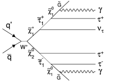
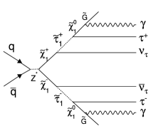
Individually, and production, as shown
in Fig. 1, contribute 45% and 25%, respectively, of
the total GMSB production cross section (). The rest of the
production is mostly slepton pairs. We note that is independent of the lifetime.
Figure 1: Feynman diagrams of the dominant
tree-production processes at the Fermilab Tevatron for the SPS 8 GMSB
model line.
The taus and second
photons, if available, can be identified as jets in the detector. Note that only one choice for the charge
is shown.
This analysis focuses on the
final state which is expected to be more sensitive to the favored
nanosecond lifetime scenario [14].
To identify GMSB events, we use the CDF II detector. As shown in Fig. 1, each gaugino
decays (promptly) to a in association with taus whose
decays can be identified as jets [15].
Whether the decay occurs
either inside or outside the detector volume depends on the decay length (and the detector size). The ’s and/or the ’s leaving
the detector give rise to since they
are weakly interacting particles (the neutrinos in the event also
affect the ).
Depending on whether one or
two ’s decay inside the detector,
the event has the signature of high energy or , often with one or more
additional particles from the heavier sparticle decays. These are identifiable as an additional jet(s) in the detector. We do not require
the explicit identification of a tau. This has the advantage of reducing the model dependence of our results, making them applicable to other possible gaugino decay models.
A study to see if there is additional sensitivity from adding
identification to the analysis is in progress.
The arrival time of photons at the
detector allows for a good separation between nanosecond-lifetime
’s and promptly produced standard model
(SM) photons as well as non-collision backgrounds.
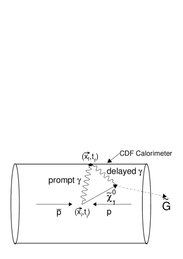
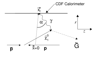
Figure 2(a) illustrates a decay
in the CDF detector after a macroscopic decay length.
A suitable timing separation variable is
(1)
where is the time between the collision and the
arrival time of the photon at the calorimeter, and is
the distance between the position where the photon hits the detector and
the collision point. Here, is the photon arrival
time corrected for the collision time and the time-of-flight. Prompt photons will produce
while photons from long-lived particles will appear “delayed”
(), ignoring resolution effects.
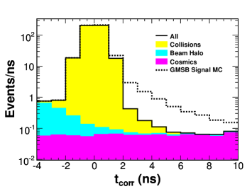
Figure 2(b) shows the simulated distribution of for a GMSB signal, prompt photons, and non-collision
backgrounds in the detector.
Figure 2: (a) The
schematic of a long-lived decaying into a and a
photon inside the detector. While the leaves undetected
the photon travels to the detector wall and deposits energy in the
detector. A prompt photon would travel directly from the collision
point to the detector walls. Relative to the expected arrival
time, the photon from the would appear “delayed.”
(b) The distribution for a simulated
GMSB signal at an example point of = 100 and
= 5 ns as well as for standard model and non-collision backgrounds.
I.2 Overview of the Search
This search selects photons with a delayed arrival time from a sample
of events with a high transverse energy () isolated photon,
large , and a high- jet
to identify
gaugino cascade decays.
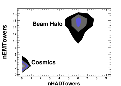
The background to this search can be separated into two
types of sources: collision and non-collision backgrounds. Collision
backgrounds come from SM production, such as strong interaction (QCD) and
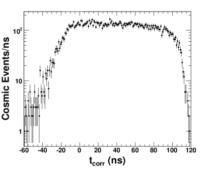
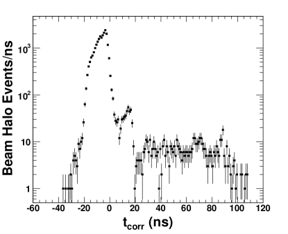
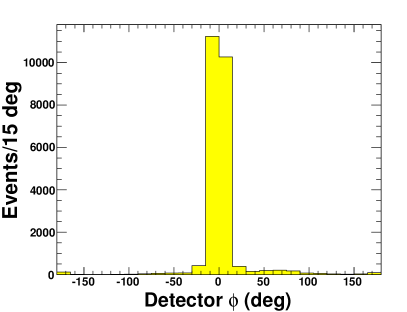
electroweak processes. Non-collision backgrounds come
from photon candidates that are either emitted by cosmic ray
muons as they traverse the detector or are from
beam related backgrounds that produce an energy deposit in the calorimeter
that is reconstructed as a photon.
The search was performed as a blind analysis, picking the final
selection criteria based on the signal and background expectations alone.
The background rates in the signal region are estimated using
control regions from the same data sample
and comparing to the distribution shapes of the various backgrounds.
A Monte Carlo (MC) simulation is used to model the GMSB event dynamics
and timing in the detector and to estimate the signal expectations.
Combining these backgrounds and signal event estimates permits a calculation of the most
sensitive combination of event requirements.
We note that the jet requirement helps make this search
sensitive to any model that produces a
large mass particle decaying to a similar final state.
I.3 The CDF II Detector and the EMTiming System
The CDF II detector is a
general-purpose magnetic spectrometer, whose detailed description
can be found in [8] and references therein. The salient
components are summarized here.
The magnetic spectrometer consists of tracking devices
inside a 3-m diameter, 5-m long superconducting solenoid magnet
that operates at 1.4 T. A set of silicon microstrip detectors
(SVX) and a 3.1-m long drift chamber (COT) with 96 layers of sense wires
measure the position () and time () of the
interaction and the momenta of charged particles. Muons
from the collision or cosmic rays are identified by a system of drift
chambers situated outside the calorimeters in the region with
pseudorapidity . The calorimeter consists of
projective towers ( and ) with electromagnetic and hadronic compartments and
is divided into a central barrel that surrounds the solenoid coil
() and a pair of end-plugs that cover the region
. Both calorimeters are used to identify and measure
the energy and position of photons, electrons, jets, and .
The electromagnetic calorimeters were recently instrumented with a new
system, the EMTiming system (completed in Fall 2004), which is
described in detail in [16] and references therein. The
following features are of particular relevance for the present
analysis. The system measures the arrival time of electrons and photons in
each tower with using the
electronic signal from the EM shower in the calorimeter.
In the region , used in this analysis,
photomultiplier tubes (PMTs) on opposite azimuthal sides of the
calorimeter tower
convert the scintillation light generated by the shower into an
analog electric signal. The energy measurement integrates the charge over a 132 ns timing window around the collision time from 20 ns before the collision until 110 ns afterwards. New electronics inductively branches off
15% of the energy
of the anode signal and sends it to a discriminator.
If the signal for a tower is above 2 mV (3-4 GeV energy deposit),
a digital pulse is sent to a time-to-digital converter (TDC) that
records the photon arrival time and is read out for
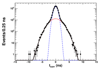
each event by the data-acquisition system. The resolution of the time of arrival measurement is ns for the photon energies used in this analysis.
II Photon Identification and Timing
The CDF detector has been used for the identification (ID) of
high-energy photons for
many years, and a standardized set of ID criteria (cuts) for the region
is now well established. Each cut
is designed to separate real, promptly produced
photons from photons from decays, hadronic jets, electrons, and other backgrounds,
see [7, 9, 17] for more details and the Appendix for a description of the ID variables.
Unlike photons from SM processes, “delayed” photons from long-lived
’s are not expected to hit the calorimeter coming directly from
the collision point [14].
As shown in Fig. 2(a), ’s with a long lifetime and small boost can produce a photon from with a large
path length from the collision position to the calorimeter (large ).
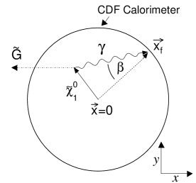
We define the photon incident angle at the face of the EM calorimeter,
, as the angle between the momentum
vector of the photon from the and the
vector to the center of the detector.
For convenience we consider the projection onto
the ()-plane and label it , and the projection onto the
()-plane and label it ; see Fig. 3.
This distinction is made as the photon ID variable efficiencies vary
differently between and .
Figure 3: The definitions of the and
incident angles using schematic diagrams of a long-lived decaying to a photon and a in the CDF detector.
The angles and are the projections of the
incident angle at the
front face of the calorimeter in the (,)- and the
(,)-plane, respectively.
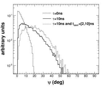
Figure 4: The
distribution of the
total incident angle at the front face of the
calorimeter for simulated photons from ’s
with = 110 . “Prompt” photons from ’s with a
lifetime of 0 ns (solid) are compared to photons from ’s with
a lifetime 10 ns (dashed). The dotted histogram shows the
distribution for a lifetime of 10 ns for photons with
ns and shows that, as expected, delayed photons can have a significant incident angle.
Figure 4 compares the distribution
for prompt, SM-like photons and photons from long-lived ’s.
Each are simulated as the decay product of a with = 110 using the pythia
MC generator [18].
The distributions of promptly produced photons [19]
have a maximum at =0∘ and extend to 18∘ in while is always
as the beam has negligible extent in the - plane.
The most common angle
for a simulated neutralino sample with = 10 ns is 10∘ and extends out
to maximum angles
of 60∘ and 40∘ in and respectively. For this sample,
the majority of photons arrive at angles between 0 and 40∘ total
incident angle. The mean of the distribution rises as a function of
but becomes largely independent of and
in the range ns.
Also shown is the distribution for delayed photons, selected with
ns, similar to a typical final analysis requirement.
The delayed photon requirement shifts the maximum of the
distribution of from 10∘ to 25∘. As the incident angles
of photons from long-lived particles are much larger than for prompt
photons, the standard selection criteria are re-examined and modified
where necessary.
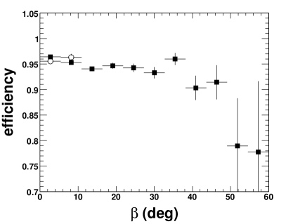
To verify that we can robustly and efficiently identify
photons from heavy, long-lived particles,
we examine the efficiencies of the
photon ID variables as a function of and separately.
As we will see
the standard photon identification requirements are slightly modified
for this search; each is listed in Table 1.
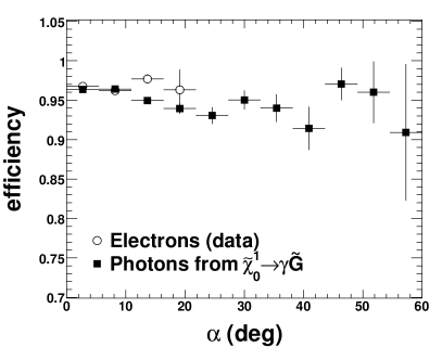
To study photon showers at a wide variety of angles in the
calorimeter, we create a number of data
and MC samples of photons and electrons. An electron shower
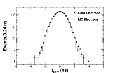
in the calorimeter is very similar to that from a photon, but electrons can be selected with high
purity. We create two samples of events, one from data, and the
other simulated using the pythia MC generator and the standard, geant based, CDF
detector simulation [20]. Each must pass
the requirements listed in Table 2.
Similarly, two samples of MC photons
are generated using decays
with = 110 and = 0 ns and = 10 ns
respectively to cover the region . The highest photon in the event is required to be the decay product of a
and to pass the , , and fiducial requirements listed in
Table 1.
GeV and
Fiducial: not near the boundary, in or , of a
calorimeter tower
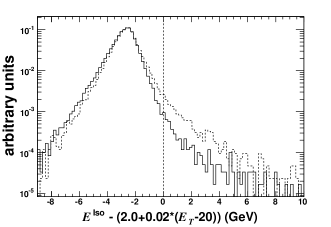
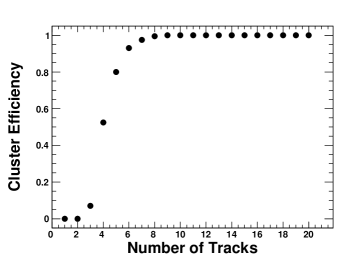
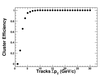
Energy in a cone around the photon
excluding the photon energy:
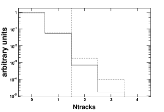
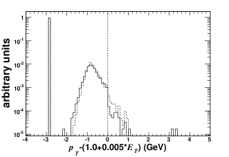
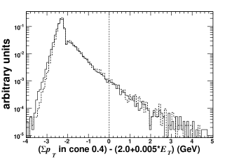
No tracks pointing at the cluster or
one with
of tracks in a 0.4 cone
Table 1: The photon identification and isolation selection requirements. These are the standard requirements with the requirement removed.
These variables are described in more detail in [9, 17] and the Appendix.
Electron Requirements
GeV and
Fiducial: not near the boundary, in or , of a
calorimeter tower
or
Track traverses 3 stereo and 3 axial COT
superlayers with 5 hits each
Additional requirements to reject electrons from
Global Event Requirements
30 GeV
Exactly 1 vertex with and cm
Transverse mass of the electron and :
Table 2: The requirements used to
select electrons from events to validate
the ID efficiency of simulated photons.
These are topological and global
event cuts in combination with loose calorimetry but tight track
quality requirements.
This produces a sample that
contains electrons with high purity but has a low bias for
calculating the efficiency of photon ID requirements vs. incident angle.
The vertex reconstruction algorithm is described in
Section II.1 and uses tracks passing the
requirements listed in Table 3. These
variables are summarized in the Appendix and described in more
detail in [8].
Figure 5 compares the distributions of the photon ID
variables for the = 0 and = 10 ns samples. A visual comparison shows that
the differences are, on average, very small.
Figure 5: A simulation of the ID variable distributions (minus their requirement value) for photons in
a GMSB model with = 110 .
The solid line is for prompt
photons, simulated as decay photons from ’s with a lifetime
of 0 ns and the dashed line is for photons from
long-lived ’s with a lifetime of 10 ns.
Entries to the left of the dashed vertical line pass the
corresponding requirement. The bin at in (d)
collects the photons that have no track within the isolation cone.
In (f) the bin at
shows the photons that have no 2nd CES cluster nearby.
The distributions for
all ID variables do not change significantly between the prompt
and the long-lived case except for slight deviations in the energy
isolation in (b) as discussed in the text.
Figure 6
shows the efficiency of the final set of ID requirements for MC photons and electrons from data as a function of incident
angles and (taking the photon position from the measured center of the calorimeter energy cluster). The efficiencies are very similar and constant except at large values
of where the efficiency drops, which is where real collision data are not
available. The drop in efficiency at large is due to the photon
shower in the calorimeter traversing into
the neighboring tower in . Because the photons are identified
and measured as clusters in the calorimeter [17], this
decreases the cluster-energy sum while increasing the isolation
energy. Therefore, the photon
appears non-isolated and the isolation efficiency falls from
98% at = 0∘ to 90% at = 50∘. This is not a
problem for large as energy leakage into the neighboring tower in
is included in the energy sum. The total photon identification
efficiency as a function of in this regime falls from
93% to 80%. However, since in our region the
fraction of events with
large is small (see Fig. 4), even at large ,
the ID criteria are only 1.5%
less efficient for photons for the = 10 ns sample than for the prompt sample.
Thus, the majority of the standard
requirements are not changed for the search. The efficiency variation as a
function of angle is taken into account
by using the detector simulation for the efficiencies and
assigning a 5% systematic
uncertainty to the overall photon ID efficiency measurement.
Figure 6: The
efficiencies for photons and electrons to pass the ID requirements
in Table 1 vs. incident angles and . The
solid squares represent MC
photons from decays ( = 110 , = 10 ns) while
the empty circles represent electrons from a data sample that pass the
requirements in Table 2. The efficiency
falls by 15% from 0∘ to 60∘ in . This effect is mostly
due to the energy isolation requirement, as discussed in the text.
The comparison of the photon shower-maximum profile to
test-beam expectations, [17], is removed
from the photon
identification requirements because it becomes inefficient at large angles.
The shower for a photon that hits the shower-maximum detector (CES) at a
large value of () angle would spread out and have a
larger-than-expected RMS in the ()
direction due to the projection. A geant simulation [20] shows the efficiency of the
requirement is constant at small angles, but then falls off
rapidly at large
angles. Thus, the photon requirement is removed.
Figure 7: A comparison of the PMT
asymmetry, , for a photon+ sample that contains both PMT
spikes and real photons,
and a sample of electrons
from events.
PMT spikes can be effectively removed by
requiring the asymmetry to be less than 0.6.
A second change to the standard photon ID is to add a requirement to remove high-energy
photon candidates that are caused by a high-voltage
breakdown (“spike”) between the PMT photocathode and the surrounding
material. Such an occurrence can produce false photon candidates that
are uncorrelated with the collision and appear delayed in time.
Spikes are identified by the
asymmetry of the two energy measurements of the PMTs of a tower:
(2)
where and are the two PMT energies. Figure 7 compares photon candidates from both
real photons and spikes to real electrons from events. The
photon candidates pass all but the identification
requirements shown in Table 1 in events with
GeV, while the electrons selected pass the requirements
in Table 4.
As shown in the figure, a requirement of
rejects 100% of all spikes with a minimal loss in effeciency for real photons. Thus, this source will be neglected in the background estimate.
II.1 Measurement of the Collision Time and Position
The corrected photon time is a combination of the measurements of the photon arrival time and position
using the EMTiming system and the primary interaction position and time
using the COT. We begin with a description of a new vertexing
algorithm that provides this time and continue with the EMTiming
measurement and the final calculation.
The standard vertexing algorithms [22] reconstruct the
vertex position () from high quality COT and SVX tracks.
However, it is important also to measure and
to separate tracks from the vertex that produced the photon from any other vertex that lies
close in space but occurs at a different time. This is
particularly true at high instantaneous luminosities where two or
more collisions can occur in one event and can lie close to each other
in . Misassigned vertex events are a dominant
contribution to the background estimate.
or passes the slow proton rejection cuts
if charge
cm
cm
ns
ns
Traverses 3 stereo and 3 axial COT
superlayers with 5 hits each
Table 3: The set of
requirements for tracks to be included in the vertex
reconstruction. These are the standard tracking
requirements [8],
but with additional quality
requirements on the measurement and a
slow proton rejection requirement [21]
to remove tracks that likely have a mis-measured track
. These variables are described in the Appendix.
GeV and
Fiducial: not near the boundary, in or , of a
calorimeter tower
and cm
cm
or
Track traverses 3 stereo and 3 axial COT
superlayers with 5 hits each
Table 4: The identification requirements for use in selecting electrons with high purity to study the vertexing performance. Note that “” is the
charge of the electron. The identification requirements are
summarized in the Appendix and described in
more detail in [8].
To solve this problem, we have developed a new vertex reconstruction
algorithm based on track clustering. The procedure [23] uses tracks with a
well measured and that pass the requirements in
Table 3 and groups those
that are close to each other in both space and time. The algorithm can
be separated into three phases: (1) the initial
assignment of tracks that are nearby in and into
clusters, (2) the determination of the , , and of
the vertex,
and (3) the adjustment of the
number of clusters by merging clusters that are close
to each other.
A simple algorithm is used to make a preliminary assignment of all tracks into clusters. It is designed to overestimate, initially, the number of vertices in the event to obviate the need for dividing a single cluster into two separate clusters, called splitting. The highest- track is designated as the “seed” of the first cluster, and
any lower- tracks that lie within three times
the typical cluster RMS (0.6 ns
and 1.0 cm for and , respectively) are also assigned to it. The highest- track
from the remaining set of tracks is then picked as a second seed and
tracks are assigned to it, and so forth until no tracks are left.
The mean position and time for each cluster,
and respectively,
is then calculated.
The vertexing algorithm is essentially a likelihood fit
using an iterative procedure to get a best estimate of the true number
of vertices and their parameters [24]. We allow the cluster parameters to float in the fit and maximize the probability that each track is a member of a vertex with a track density that is Gaussian in both space and time.
All clusters are fitted simultaneously.
If during the procedure the means of two clusters are within
both 3 cm in and 1.8 ns in or if two clusters share the same set
of tracks, then the clusters are merged.
No splitting is done because
the initial seeding is designed to
overestimate the number of clusters. Splitting a cluster
with a too-large RMS can result in two clusters that both do not
pass the final requirements and would reduce the clustering
efficiency. Having two clusters merged that are close in both space
and time does not substantially affect the measurement. We choose the primary
vertex for an event to be the highest cluster that has at least 4
tracks.
II.1.1 Vertexing Resolution and Efficiency
The cluster resolution, the reconstruction
efficiency, and beam properties are measured using a high purity data
sample, selected using the cuts in Table 4.
To measure the performance for possible events with photons,
the electron track is removed from the vertexing and is used to measure
the vertexing performance as it identifies the correct event vertex.
Figure 8 shows the
and distributions as well as their correlation for the vertices in this sample. Both are roughly Gaussian and
centered at zero with an RMS of 25 cm and 1.28 ns, respectively,
reflecting the accelerator performance. There is a non-Gaussian excess around
zero in the distribution that comes from events that contain more than one vertex. In this
case the clustering has merged two vertices that are close to each
other, which most likely happens at cm. The correlation between the collision position and time distributions is caused by the differences in the proton and anti-proton bunch structure within the accelerator
( cm and
cm [7]).
Figure 8: Plots (a), (b), and (c) show the ,
, and their correlation respectively for the reconstructed highest vertex in events. The fits in (a) and (b) are both a single Gaussian.
The falloff in the (b) at cm is due to the
requirement that all tracks have cm.
In the search the vertex is
required to have cm.
The vertexing resolution is estimated using a subsample of the events with only one
reconstructed vertex. For each
event the tracks in the vertex are randomly divided into two
groups that are then separately put through the vertexing algorithm.
Figure 9 shows the distance between the two clusters,
divided by to take into account the two measurements,
giving a resolution measurement of ns and
cm.
The secondary Gaussian in Fig. 9(b) indicates
cases where two different vertices have been combined into one cluster.
Figure 9: The difference in and between
two arbitrarily selected sets of tracks from the same
reconstructed vertex in a dataset with the electron track
removed from the vertexing. This is a measure of the vertex
resolution. (a) is fit with one Gaussian while (b) is fit with two. Note that the factor of is already taken
out.
Figure 10
shows the difference in time and position between the reconstructed
cluster and the electron track (not included in the vertexing)
for the full sample. The distributions are well described by two Gaussians that are both
symmetric and centered at zero, indicating no measurement bias. The
primary Gaussian distribution contains events where the reconstructed
cluster is the vertex that produced the electron. Its RMS is dominated
by the resolution of the electron track position and time. The
secondary Gaussian distribution contains events where the electron
does not originate from the highest vertex in the event.
Figure 10: The difference in (a) and in
(b) between the electron track and the highest reconstructed
vertex (without the electron track participating in the vertexing) in events.
The distributions are centered at zero and fit with double Gaussians, indicating that there is
no bias in the clustering procedure. The secondary Gaussian
contains events where the electron does not originate from the highest
vertex in the event.
The efficiency of the vertex reconstruction algorithm is investigated
using two separate methods. The efficiency as a function of the number
of tracks is determined by selecting events that contain a cluster
with a high track multiplicity. Next, various random subsets of the tracks are taken that belong to
this cluster to see if they alone could produce a cluster.
Figure 11 shows the ratio of
subset samples in which a cluster is reconstructed to
all cases tried for a given set of tracks as a function of the number
of tracks in the various subsets. The algorithm
is over 90% efficient if 4 tracks are present, where the inefficiency
is usually caused by the algorithm reconstructing two separate clusters each with
4 tracks, and 100% efficient with 6 tracks (the
final analysis requires at least 4 tracks).
A second method that also allows for a measurement of the efficiency
as a function of the is to consider tracks in a window around the electron track
(5 in each direction) and search for clusters.
Only events with at most one reconstructed vertex are considered.
While this result is not biased by
selecting cases with a known vertex, the disadvantage is that
for resolution reasons not
all tracks are in the window, resulting in a
small under-counting of the number of tracks. Figure 11
shows that the efficiency as a function of the number of tracks in the
vertex yields a similar result for the two very different methods.
This gives confidence in the results as a function of
. The efficiency plateaus at , as higher tracks have a better resolution measurement.
It is important to note that the efficiency measurements
as a function of the number of tracks are sample-dependent.
For instance, if a sample is chosen that is biased towards a higher
average track then the efficiency might be higher for a smaller
number of tracks, or if a sample contains many high- tracks,
the efficiency as function of might plateau earlier. Since the
search requires , as
stated later, we take the efficiency for the vertex selection
requirements to be 100%.
Figure 11: The clustering efficiency as a
function of the number of tracks using (a) the subset method and
(b) the window method, and (c) as a function of the of the
tracks using the window method. Note that a cluster is required to have at least 4 tracks and the
efficiency is 100% for in this search.
II.2 The Corrected Photon Time
With the vertex time and position in hand, we move to a full measurement
of by incorporating the EMTiming information.
The time of arrival recorded by the EMTiming system TDCs
is corrected using calibrations
that take into account
channel to channel variations and an
energy-dependent (“slewing”) effect due to the fixed-threshold discriminators. A full description of the hardware as well as the correction and calibration
procedure is described in Ref. [16].
The resolution
for electrons from events is 0.64 ns (0.63 ns) for collision data (MC),
dominated by the intrinsic resolution (0.5 ns), the precision of the
TDC output (0.29 ns) and the vertex resolution (0.22 ns).
A comparison of detector simulation to collision data for events is shown in Fig. 12. There are no non-gaussian tails out to .
Figure 12: A
comparison between MC (solid) and collision data (points) for for electrons from a sample.
The distributions are well
centered around 0 and the resolutions of collision data and MC fit well with
a fully corrected RMS of 0.64 ns.
III Triggers, Datasets and Event Preselection
The event selection is a three stage process. The stages are (1) an
online sample is selected (during data taking), (2) a “preselection sample”
is selected offline, and (3) the event selection uses optimized
final event selection requirements.
The full set of requirements that determine the preselection sample
for the search are summarized in Table 5. The
optimization and final event requirements are described in
Section VI.
The analysis begins by selecting events online using a single set of
3-level trigger requirements that
require a photon candidate and .
The Level 1 trigger requires
a single tower in the calorimeter with , GeV,
GeV, and GeV.
For a description of the ID variables, see the Appendix.
The Level 2 trigger requires the event to have an EM cluster with
GeV and GeV.
At Level 3 the requirements are tightened with GeV,
, and 25 GeV.
The data consist of events from the data-taking
period from December 2004, when the EMTiming system became fully
functional, until November 2005. The data
correspond to an integrated luminosity of
(57034) pb-1.
The sample of candidate events that pass the trigger requirements is
processed offline where the event
characteristics are refined to increase the signal purity and
further reduce the backgrounds. The offline preselection requirements
include photon ID and requirements as well as jet, vertex, and
cosmic ray rejection requirements. To ensure that all signal events would have passed the trigger with 100% efficiency
each event is required to have GeV, a photon with
GeV, and pass
the identification criteria shown in Table 1.
We require the presence of at least one jet and a high vertex in each event for the preselection sample.
This preserves the acceptance of and
production while maintaining a search strategy that is as
model-independent as possible.
While the term “jet” typically refers to the hadronization of a high
energy quark or gluon that is produced in the collision, at CDF
jets are identified as clusters of energy in the calorimeter. Hence,
the hadronic decays of taus and/or the energy deposits from electrons or photons are also efficiently reconstructed as jets.
Requiring at least a single jet with GeV and
[15] retains high efficiency and significantly
reduces non-collision backgrounds which typically only produce a
single photon candidate.
As previously mentioned, each event must also have a good space-time vertex with at least 4 good tracks and
a of at least 15 .
This allows for a good measurement and further helps reduce the non-collision backgrounds.
We also require cm and ns for tracks to be included in the vertexing
so that both the COT tracking and the calorimeter are able to produce
high quality measurements.
A cosmic ray that traverses the detector can create hits in the muon system that are not associated with tracks in the COT and deposit a photon candidate nearby in the calorimeter.
An event is rejected from the preselection sample if there are potential cosmic–ray hits in the muon chamber within 30 degrees in of the photon that are not matched to any track.
Table 6 lists the cumulative
number of events that pass each of the successive requirements to create our
preselection sample.
Photon
GeV and
Fiducial: not near the boundary, in or , of a
calorimeter tower
Energy in a cone around the photon
excluding the photon energy:
No tracks pointing at the cluster or
one track with
of tracks in the
cone
No second cluster in the shower maximum detector
or
Jet
GeV
Highest Space-Time Vertex
with:
cm
ns
Global Event Cuts
GeV
Passes cosmic ray rejection requirements
Table 5: The
requirements used to obtain the preselection sample
of events. The cosmic ray rejection cut is described in
more detail in [25]. The number of
events in the data that pass each cut are shown in
Table 6. For more detail on the ID variables, see the Appendix.
Selection
No. of Observed
Events
GeV, GeV,
photon ID and fiducial requirements
119944
Vertex with , 4 tracks
19574
1 jet with GeV and
13097
Cosmics rejection
12855
Table 6: Event reduction for the
preselection sample. For the
individual requirements see Table 5.
IV Backgrounds
Backgrounds to the signature
can be categorized into two different
classes: collision and non-collision events.
The rate that each type of background contributes to the final signal
time-window is estimated solely from collision data using control samples of
events that pass all of the final requirements excluding
timing. We define the “kinematic sample” as the events
that pass the final event requirements (summarized in
Section VI, Table 9)
except the timing requirement.
The distributions outside the timing signal region are used to
normalize each background, which is then extrapolated into the
signal time region. In this section each of the backgrounds is
described, and the signal estimation techniques are outlined.
IV.1 Standard Model Backgrounds: Prompt Photons
Prompt collision events dominate the sample and populate the region
around ns. As shown later, it is not important for this
search to distinguish further
between the various prompt photon sources. Most events are from
and events with
one jet reconstructed as a photon and with
from the mis-measurement of the photon and/or jet
in the calorimeter.
A smaller source is from
SM events where the electron is misidentified as
a photon and the leaves undetected to cause the .
In both cases these events can fall into the large signal time window due to either
Gaussian fluctuations of the timing measurement or a wrong
collision vertex selection. The latter case dominates the SM background
estimate and is more likely at high
instantaneous luminosity when there are multiple collision vertices
reconstructed.
To study the distribution for promptly produced photons, a sample of
events is selected using the requirements described in
Table 2. This sample is used for the reasons described
in Section II, and has the additional advantage that the
electron track in the COT allows for a determination of the
correct vertex. To mimic closely the vertexing for
events with photons, the electron track is dropped from the vertex
clustering. The highest- vertex is chosen as the most likely
to have produced the EM cluster (the “photon”).
Figure 13 shows the
resulting distribution and has a double-Gaussian shape. One
Gaussian comes from events where the vertex choice is correct and the
other Gaussian comes from events where the vertex choice is
incorrect [26].
Figure 13 also shows these events separated into right and wrong-vertex subsamples, selected by requiring a tight
match ( cm and ns) and anti-match between the electron
track and the vertex, respectively. In both cases the distributions
are Gaussian and centered at zero. The right vertex selection has an
RMS of 0.64 ns, reflecting the system resolution,
and the wrong-vertex selection has an RMS of 2.0 ns.
The wrong-vertex time distribution can be understood by combining
the RMS of the
time distribution without the vertex and corrections
(RMS ns)
with the
RMS of the collision distribution (RMS ns as shown in
Fig. 8): ns. The number of
events in the signal region () for prompt, SM sources
can thus be estimated by simple extrapolation from a measurement of
the timing distribution for ns.
Figure 13: The distribution for
electrons in a sample of
events. In plot (a) the two Gaussians correspond to the cases when the
highest- vertex is associated to the electron track and when
it is not. These cases can be separated by requiring a match (b) and an
anti-match (c), respectively, between the vertex and the electron track in
both space and time.
The systematic uncertainty on the number of prompt events in
the signal region is
dominated by the observed variation in the mean and RMS of the distribution as a function of the , jet , and photon
requirements. To estimate the variation, we study the distribution for samples of electrons in events for various
electron , jet and event requirements (, , and GeV).
The results are shown in Fig. 14.
The variation in the mean is up to 0.1 ns and is conservatively
rounded up to 0.2 ns. Similarly, the systematic uncertainty on the
RMS of is conservatively overestimated from a fit to
Fig. 14 to be 0.02 ns and is only a small addition.
For wrong-vertex assignments, there is an additional variation in the
distribution as a function of photon due to the
incorrect time-of-flight calculation.
Figure 15 shows the mean and the RMS
of the distribution for electrons from events where the
wrong-vertex is selected for the timing correction, as a function of
tower-. We take a systematic uncertainty
on the mean and the RMS of the wrong-vertex contribution to the distribution to be equal to the full variation. We assign values of 0.33 ns and 0.28 ns,
respectively, to these systematic
uncertainties, the latter arising from the largest variations in
Fig. 15.
Figure 14: The mean and RMS
of the distribution for electrons from various
subsamples of events where each
entry reflects a different combination of the electron , jet
and event requirements. There are slight shifts as the
these requirements vary.
While the mean of the distribution is close to
zero, the systematic variation on the mean of the primary
Gaussian of the prompt time distribution is conservatively
taken to be 0.2 ns in the background estimates.
Figure 15: The
mean and RMS of the distribution for electrons from events, where
the wrong vertex is picked, as a function of .
IV.2 Non-Collision Backgrounds
The fraction of non-collision backgrounds in the kinematic sample
that fall in the timing signal window is significant.
To study these backgrounds, we divide them into two separate sources,
cosmic ray muons and beam related backgrounds.
Cosmic ray events (cosmics) come from cosmic ray
muons that emit photons via bremsstrahlung as they traverse the detector
or produce significant ionization in a large interaction with the EM calorimeter.
Beam halo events (beam halo) are caused by beam particles (mostly
from the more intense proton beam) that
hit the beam pipe upstream of the detector and produce muons.
These muons travel almost parallel to the proton beam direction and
shower into
the EM calorimeter to create a photon candidate; see
Fig. 16. In both cases the event has significant
that is highly correlated with the photon and is uncorrelated with any collision that might occur
coincidentally at high luminosity. As cosmic ray muons
interact with the detector and produce a photon randomly in time,
their time distribution is roughly constant over the entire calorimeter
energy integration window range of 132 ns. Beam halo
“photons” typically arrive a few ns earlier than prompt photons for geometric reasons as shown in Fig. 16.
However in this case, while the rate is lower, the photon candidate
can also have a of 18 ns (and multiples later and
earlier) if the muon was created in one of the bunched beam interactions that
can occur every 18 ns in the accelerator.
Figure 16: Illustrations of a beam
halo event interacting with the detector. In both figures
the muon path is indicated with an arrow. (a) A
comparison of the time distributions of prompt collision events
with beam halo photon candidates for three example towers in
the calorimeter shows that the mean time changes
as a function of tower and is always less than zero. The
-axes are in arbitrary units.
(b) An illustration of how the beam halo interacts with the
calorimeter. The muon travels through multiple towers
in the hadronic calorimeter at high before hitting the
electromagnetic calorimeter.
The rate at which both non-collision backgrounds populate the signal
region is estimated from collision data using events with no identified
collision. The non-collision sample consists
of events with a photon that passes the photon ID criteria listed in
Table 1, GeV, and no
reconstructed vertex. This sample is used to make timing distribution
templates from pure samples of each type of non-collision background.
Beam halo events are identified
by the energy deposition of the muon as it passes through the high
towers of the plug hadronic calorimeter () and
the central EM calorimeter () towers at the same
as the photon candidate; see Fig. 16.
The muon deposits a small amount of energy in
most towers along its path. Hence,
we count the number of towers in the hadronic calorimeter
with GeV and (nHADTowers)
and the number of towers in the EM calorimeter with GeV and
(nEMTowers). The results are shown in
Fig. 17 for the full non-collision sample.
Cosmic ray candidates are easily separated from beam halo
candidates. This is because cosmics do not deposit energy in the
hadronic calorimeter with and typically only deposit
significant energy in a single EM tower. An event is identified as a
cosmic if it has nHADTowers = 0 and nEMTowers . (Note that we also ignore
all photon candidates with as beam halo dominates
there.) Conversely, beam halo events are identified if they have no
muon stubs and have both nHADTowers and nEMTowers .
The distribution for each is shown in
Fig. 18
for the entire calorimeter energy integration window and indicates that the real collision contamination is negligible.
As these events lack a vertex, the photon
arrival time is corrected assuming = 0 and = 0 in Eq. 1.
To create the distribution for use in extrapolating the number of non-collision events in the signal time window from the control regions, we
convolute
the distributions in Fig. 18 with the RMS of the interaction
time of 1.3 ns as the collision time is
uncorrelated. As will be seen, the
uncertainty on the rate of the number of events in the signal time region
is dominated by the statistical uncertainty
on the number of non-collision events in the control regions.
We note that because of the accelerator geometry there are 40
times more beam halo events that occur
around the region as can be seen in Fig. 19.
This explains the separation requirement and will
be further used in the final background estimate procedure.
Figure 17: The variables used to
separate cosmic and beam halo backgrounds in the sample without
a vertex. Beam halo muons deposit energy in many HAD towers as
they interact with the detector at high
and many EM towers as they traverse the central portion of the
calorimeter along the beam halo direction.
Figure 18: The distributions for the cosmic ray (a) and beam halo (b) backgrounds in the sample without a collision.
Figure 19: The number of beam halo photon candidates as a function of
detector .
Most photons arrive at .
IV.3 Background Estimation Methods
The number of background events in the signal region is estimated from collision data
by fitting a set of control regions with background timing shapes and extrapolating
into the signal time window. The distribution shape “templates” for
each background source are given in Figs. 13
and 18. Since a sample is defined by kinematic cuts alone
we can estimate the number of background events in any potential signal time
window using sensibly chosen control regions. Thus, we can predict the
background rate for a large variety of final kinematic and timing cuts and use
these estimates as part of our optimization procedure.
The background prediction for the signal timing region for each subsample of
events after the kinematic sample requirements is done as a two-step
process with multiple control regions. There are a number of reasons for this.
Multiple control regions are used to get a robust estimate of each of the
background event contributions that are hard to separate; for example
the timing region {} ns is populated by both
the wrong-vertex backgrounds and
beam-halo backgrounds. Secondly,
for many of the potential kinematics-only samples, low statistics can
bias the fit results. We define a set of control regions chosen such
that each is largely dominated by a single background source, and use
an iterative fitting procedure
to ensure that each background is well estimated for each kinematic
requirement choice during optimization.
The control regions are designed to allow for a good estimation of each background separately.
Since the cosmics rate is essentially constant in time, the time
control region is defined to be {} ns and is chosen such that
(a) it is well above the beam halo secondary peak at 18 ns
and (b) it does not include the region close to the end of the
calorimeter energy integration window where the event
rate falls sharply. The beam halo control region is defined to be
{} ns and is
chosen such that (a) it contains most of the beam halo events but (b)
stays well away from the region dominated by the prompt photon
production. The standard model control region is defined to be
{} ns. An additional requirement on this region is that the photon must have
. This allows us (a) to include as much of the
collision data as possible to get good precision on the
ratio of right to wrong-vertex events,
(b) allows for a potential signal
region above 1.2 ns, and (c) removes most of the beam halo
contamination. We note that while the restriction is useful for
estimating backgrounds, it is not an effective tool in improving the
sensitivity. While the upper time limit of the signal
region at 10 ns is not quantitatively motivated, it contains most of a
long-lived signal on the order of nanosecond lifetimes as the time
distribution falls exponentially (Fig. 2).
The background prediction for the signal timing region for each subsample of
events after the
kinematic sample requirements is done as a two-step
process.
In step 1, the wrong-vertex fraction and the overall prompt photon
rate are measured using the collision data control sample after a
correction for non-collision contamination.
The non-collision contamination to the control sample is estimated by
fitting the beam halo template and cosmics,
simultaneously in the control regions {} ns (beam halo
dominated) and {} ns (cosmics dominated). The fit is extrapolated to
the collision control region {} ns, where the non-collision
contamination is subtracted
off. The remaining data are then fit using the two single Gaussian functions as
shown in Fig. 13. While the mean and RMS of both
functions are fixed, the normalizations are allowed to float. After
fitting, the final normalization is scaled by a factor of 12/11 to account for the removed data in the slice around .
The statistical error on the prediction in the
signal region is determined by the fit.
The uncertainty on the number of
events in the signal time window is estimated by varying the
collision background fractions, means, and RMS’s according to their systematic and statistical uncertainties. We note that if we choose the kinematic sample to be the dataset that passes the preselection sample criteria (see Table 5), the
resulting fraction of wrong-vertex events
is (31)%.
In step 2, the rate of the non-collision backgrounds is estimated using the entire region. In the full data sample a
simultaneous fit is performed for the normalization
of the beam halo and cosmic ray backgrounds using the control regions,
after subtracting off the expected contamination from collision
sources in both regions obtained in step 1. The
uncertainties on this estimate are dominated by the statistical
error on the number of events in the control regions and the
uncertainty on the extrapolation from the prompt background. With this
technique, the background estimation for all sources is robust enough to be
applied to a variety of kinematic requirements. This feature
will be used along with the simulated acceptance of GMSB events
for the optimization.
V Acceptances For GMSB Events and Their Systematic Uncertainties
We use MC techniques to estimate the acceptance and overall
sensitivity to GMSB models.
The sparticle properties (mass, branching fractions etc.) are
calculated with isasugra [27].
Samples of events of GMSB processes are simulated according to their
production cross sections using pythia [18], a full
detector simulation, as well as parton distribution functions
(PDFs) [28]. All sparticle production mechanisms are
simulated as this maximizes the sensitivity to the
model [29].
To map out the sensitivity for GMSB models as a function of
mass and lifetime, MC samples are generated
for and ns.
As 5% of the simulated
events pass all the selection requirements,
the size of the MC samples is chosen to be 120,000 events so that
their statistical uncertainty is
1% and negligible compared to the combined systematic uncertainty.
The total event acceptance
is
(3)
where the MC program is used to estimate , the fraction of events
that pass the kinematic sample requirements and to
estimate , the fraction of
these events that remain after the requirement.
is a correction factor
for efficiency loss due to the cosmic ray rejection requirement and
is not simulated. Table 7 shows the breakdown of
the number of MC events after each of the preselection sample
requirements in Table 5 for an example GMSB point at
= 100 and = 5 ns, near the expected sensitivity limit.
The loss of signal events due to the cosmic ray rejection requirement is
chiefly caused by real cosmic rays overlapping the
signal events and causing the requirement to fail.
This efficiency is estimated simply to be equal to the efficiency of the
requirement as measured from the preselection sample but
additionally requiring the
photons to be within ns to select collision events with
high purity. There are 12,583 events in this sample.
12,360 events remain after the cosmic ray rejection requirement,
giving an efficiency of
%, with the error
conservatively overestimated.
Requirement
Events passed
(%)
Sample events
120000
100.00
Central photon with
GeV, and
GeV
64303
53.6
Photon fiducial and ID cuts
46730
38.9
Good vertex
37077
30.9
1 jet with GeV
and
28693
23.9
Cosmic ray rejection ()
N/A
23.5
Table 7: Summary of the MC event reduction for a GMSB example point at
= 100 and = 5 ns as a function of the preselection
sample cuts of Table 5. Note that the efficiency
loss caused by the cosmic ray rejection
requirement is implemented as an MC correction
factor, .
The systematic uncertainty that enters the limit
calculation (and thus a proper optimization) is dominated by the
potential shift of the measurement
for the kinematic sample requirements.
This along with the remaining systematic effects on the acceptance,
luminosity, and production cross section are summarized in
Table 8. The uncertainty is evaluated at
and ns.
The effect of varying and is negligible when compared
to the other systematic effects.
We next describe the estimation of these important effects.
Relative
Factor
Systematic
Uncertainty (%)
Acceptance:
measurement and vertex selection
6.7
Photon ID efficiency
5.0
Jet energy scale
1.0
Initial and Final State Radiation
2.5
Parton Distribution Functions
0.7
Total
8.8
Cross section:
Parton Distribution Functions
5.9
Renormalization scale
2.4
Total
6.4
Luminosity
6.0
Table 8: Summary
of the systematic uncertainties on the acceptance and the total
production cross section.
•
Time measurement:
There is an uncertainty on the acceptance due to the systematic variations
in the measurement shown in Fig. 13. Three types of uncertainties are considered
simultaneously: (1) a shift in the mean
of measurement, (2)
a change in the RMS variation of the measurement, and (3) a change in the
fraction of events that have an incorrectly chosen vertex.
The variation of the mean of
the right (wrong) vertex measurement has been conservatively
overestimated to be 0.2 ns (0.33 ns) and can shift events into and
out of the signal region. The fractional variation in acceptance due
to this effect is estimated to be 6.7%.
The fractional change in acceptance due to changing the RMS of the measurement
is estimated to be 0.03%.
The variation due to fluctuations in the number of additional vertices,
is 1.5% [30].
Taken in quadrature the total uncertainty is 6.7% and
forms the dominant contribution to the systematic uncertainty on the
acceptance.
•
Photon ID efficiency:
As described in Section II, the systematic uncertainty
on the photon ID efficiency is estimated to be 5%.
•
Jet energy:
As the event selection requires a jet with GeV
a systematically mismeasured jet can contribute to the acceptance
uncertainty.
We use the standard CDF procedure [15] of varying the jet energy
by of the estimated energy systematic uncertainty and find the resulting variation in the acceptance to be 1.0%.
•
Initial and final state radiation:
The uncertainty in the MC simulation of ISR and FSR effects can cause
the photon, the jet, or
the to be systematically more likely to pass or fail the kinematic
sample requirements and affect the acceptance. This is estimated using the
standard CDF procedure of varying the ISR/FSR parameters as
described in [22].
The systematic variation in the acceptance is estimated to be 2.5%.
•
Parton distribution functions (PDFs):
The production cross section and the acceptance have uncertainties
due to uncertainty in the PDFs. The uncertainty is estimated using the
standard CDF procedure of varying the PDFs within the uncertainties
provided by cteq-6m as described in [28].
We find a relative uncertainty of % on the
acceptance and % on the cross section.
•
Renormalization scale:
There is a systematic uncertainty of the NLO
production cross section which is estimated using the standard technique
of varying the renormalization scale between 0.25
and 4 using prospino2 [31]. The variation of
the cross section is estimated to be 2.4%.
VI Optimization and Expected Search Sensitivity
The sensitivity to sparticle production is estimated in the
form of the expected 95% C.L. upper cross section limits
() for various points in parameter space.
Before unblinding the signal region in the data we optimize the
search sensitivity and determine the best event selection requirements for a
prospective GMSB signal. This is done using the background rates
and the signal acceptances for all sparticle production, with uncertainties,
available for different sets of selection requirements.
The procedure is to consider the number of events “observed” in a
pseudo-experiment, , assuming no GMSB signal
exists, and to calculate
using a Bayesian method with a
constant cross section prior [32].
The uncertainties on the signal efficiencies,
backgrounds, and luminosity are treated as nuisance parameters with
Gaussian probability distributions.
We write
since the limit is also a function of the number of predicted
background events and ,
where both factors depend on the set of requirements (cuts) used.
The expected cross section limit is calculated from
and takes into account the
outcomes of the pseudo-experiments determined by their
relative Poisson probability [33], .
The expected cross section limit and its RMS are given
by:
(4)
(5)
where is the number of expected background
for a given set of cuts and (,) is the normalized Poisson distribution of
with a mean .
The expected maximal sensitivity for each GMSB parameter choice is
found when the set of requirements
minimizes .
To find the minimal
we simultaneously vary the photon , , and jet
thresholds, , and the lower limit on . Here is
the azimuthal angle between and the
highest- jet. This angle cut helps reject events where the is
overestimated because of a poorly measured jet.
The upper limit on is kept constant at 10 ns.
As an illustration of the optimization,
Fig. 20 shows the
expected cross section limit for a GMSB example point [12] at
= 100 and = 5 ns as a function of the lower
requirement. All other requirements are kept fixed at
their optimized values. This point is close to the boundary of the
exclusion region.
Figure 20: The expected 95% C.L. cross section limit as
a function of the lower value of the requirement
for a GMSB example point with = 100 and = 5 ns. The values of the kinematic sample requirements
are held at their optimized values.
In the region ,
ns the optimal cut values have negligible variation except for a small variation in the optimal jet requirements and the lower limit on .
A single fixed set of final requirement values is chosen since, far
from the expected exclusion boundaries, this results in at most a
4% loss of sensitivity.
The final values are Photon GeV, jet GeV,
, GeV, and ns.
For and ns we find an acceptance of (6.30.6)%.
Table 9 gives more details on the acceptance reduction
as a function of the requirements.
Our fit to the data outside the signal region predicts total backgrounds of
6.23.5 from cosmic rays, 6.84.9 from beam halo background
sources, and the rest from the standard model with a measured wrong-vertex fraction of (0.50.2)%. Inside the signal region, ns, we predict 1.250.66 events: 0.710.60 from
standard model, 0.460.26 from cosmic rays, and 0.070.05 from
beam halo.
Table 10 shows
the various possible number of “observed” events and their probability in the no-signal hypothesis.
We find for this point in parameter space fb with an RMS of 42 fb.
The total sparticle production cross sections, ,
are calculated at next to leading order (NLO) by multiplying the
LO production cross section from pythia [18] by the
theoretical K-factors from [34] (1.2 for this mass range).
A total sparticle production cross section of 162 fb is predicted for this
point, and thus we expect to exclude it. A total of 5.70.7
signal events is expected for this mass/lifetime combination.
Preselection Sample
Individual
Cumulative
Requirements
Efficiency
Efficiency
(%)
(%)
GeV, GeV
54
54
Photon ID and fiducial,
74
39
Good vertex,
79
31
, GeV
77
24
Cosmic ray rejection
98
23
Requirements after
Optimization
GeV, GeV
92
21
(, jet) 1.0 rad
86
18
2 ns 10 ns
33
6
Table 9: The data
selection criteria and the total, cumulative event efficiency
for an example GMSB model point at = 100 and
= 5 ns. The listed requirement efficiencies are in
general model-dependent. The good vertex requirement (95%
efficient) includes the cm cut. The efficiency of
this cut, as well as that of
the photon fiducial and cosmic ray rejection cuts, is
model-independent and estimated from data.
(fb)
Probability (%)
0
79.9
28.7
1
120
35.8
2
153
22.4
3
196
9.32
4
239
2.91
5
280
0.729
Table 10: The 95% C.L. cross
section limit as a function of the hypothetically observed
number of events, the Poisson probability for the number of
events based on the no-signal hypothesis (1.3 events expected) at an example GMSB point of =100 and =5 ns, and the requirements listed in Table 9. We find for this point in parameter space fb with an RMS of 42 fb. A total sparticle production
cross section of 162 fb is predicted for this
point, and thus on average we expect to exclude it.
Control Region
Dominant Background
Observed Events
ns
Beam halo
4
ns
SM
493
ns
Cosmics
4
Table 11: The observed number of events in
each control region after all the optimized kinematic sample requirements.
VII Data, Cross Section Limits and Final Results
After the kinematic requirements (Table 9) 508
events remain in the
data sample. Table 11
lists the number of events observed in
the three control regions. Figure 21 shows the
distribution
from data along with the signal expectations and the background
shapes, normalized using the control regions.
Figure 21: The distribution including the control and signal regions, after all but
the timing cut for all backgrounds, for the expected signal and the
observed data. A total of 508 events is observed in the full time
window. The two observed events in the signal region,
ns, are in the first signal time bin (marked with a
star). This is consistent with the background
expectation of 1.30.7 events.
Since the number of events in the timing window ns is predicted by the background estimation techniques we can compare the number of predicted and observed events. Table 12 shows the results as each
of the optimized requirements is applied sequentially along with the expectations for a GMSB example point.
The large fractional errors on the backgrounds
are due to the systematic uncertainty on the mean and RMS of the SM
distributions as discussed in Section IV.
The large fractional errors on the beam halo and
cosmic ray estimates are primarily due to the small
number of events in the
control regions. Neither is a problem in the final analysis as the absolute number of background events is small in the signal region.
After each requirement, sparticle production would have increased
the number of events observed in the signal region above the
background levels. However, there is good
agreement between the background prediction and the number of events
observed in all cases. The bulk of the beam halo and cosmics background are rejected by the timing
requirement.
There are 2 events in the final signal region,
ns, consistent with the background expectation of
1.30.7 events.
Figure 21(b) shows in detail the
time window immediately around the signal region. The data is consistent with
background expectations. The two events have of 2.2 ns and
2.6 ns respectively. Figure 22 shows the
distributions for the background and signal expectations along with the data as
functions of the photon , jet , , and requirements.
There is no distribution that hints at an excess.
Requirement
Expected Background
Expected
Data
SM
Beam Halo
Cosmics
Total
Signal
Photon, , jet pre-
selection cuts and
ns
490.74295.40
0.270.12
1.300.49
492.3295.4
11.71.4
398
GeV
162.9676.19
0.240.12
1.170.46
164.476.2
10.21.2
99
Jet GeV
154.5272.96
0.120.08
0.790.37
155.473.0
9.41.1
97
13.0711.57
0.100.07
0.520.30
13.711.6
8.51.0
8
ns
0.710.60
0.070.05
0.460.26
1.30.7
5.70.7
2
Table 12: Summary of the expected and
observed number of events from the background estimate after the
preselection sample requirements and each requirement from
the optimization,
separated for each background, and the expected number of signal
events. The expected signal numbers
are for a GMSB example point at = 100 and
= 5 ns. Note that the additional requirement
ns is applied at the top line to allow the
background estimation methods to use the prompt control region to make
predictions at each stage. The preselection sample cuts are listed in
Table 5. The background predictions match well
with the observed number of events for each requirement
indicating the background estimation methods are reliable. There
is no evidence of new physics.
Figure 22: The predicted and
observed photon , jet , , and distributions
for the signal region after the
final event selection requirements. The GMSB distributions are for
= 100 and = 5 ns.
There is no evidence for new physics.
A model-independent exclusion limit can be assigned based on this
non-observation. The two observed events and the background and its
uncertainty give a 95% C.L. upper limit () on the
number of events produced of events.
Any model of new physics that predicts more than this number of
delayed events is excluded.
To make our results useful for future model builders to calculate cross section limits for other acceptance models, we calculate
a correction factor, , that takes into account the systematic uncertainties on the acceptance, efficiency and
the luminosity, which are also fairly model-independent. Using the relation
(6)
and the methods to calculate ,
we find = 5.5 events.
VII.1 Cross Section Limits and Exclusion Regions for GMSB Production
To compare our results to GMSB models we calculate the 95% C.L. upper limits and compare to GMSB production cross sections.
To allow for a more detailed comparison to
production cross sections for any other model that predicts heavy, long-lived,
neutral particles that produce the final state [35] we parametrize the acceptance using variables that are largely independent of
the GMSB specific dynamics.
There are several effects that
cause the acceptance to vary as a function of both the mass and
lifetime. The dominant ones are the probability that (a) at least
one of the two decays in the detector volume
to produce a photon that passes the kinematic sample selection criteria
() and that (b) is within the signal time
window ().
We find these are roughly independent of each other,
and define , where is a minor
correction described below.
We find:
(7)
(8)
where each function consists of two multiplicative terms: a
mass-dependent term that determines the overall scale, and a lifetime
dependent term. Here is in and is in ns. The small
mass dependency of the
overall scale and of the exponential term in both
come from variations in the boost with its
mass in production [14]. A higher boost can cause
the to leave the detector with a higher probability given its
lifetime and cause the photon to be emitted at smaller angles relative
to the direction such that its arrival time becomes similar to a promptly
produced photon. A variation in the boost is caused by a change in the
shape of the distribution as a function of
the mass. Another important, but non-dominant, factor is the
lifetime term
in the denominator of both exponentials. This takes into account the
effect that both the acceptance and efficiency are not zero at low lifetimes but have a finite contribution due to the resolution of the measurement. This causes prompt photons to fluctuate into the signal
time window.
An additional lifetime dependent correction term, , is
introduced to compensate for remaining small deviations in
:
(9)
where is in ns. This simple parameterization well characterizes the acceptance for any GMSB model to better than 4% and gives us confidence that it can be of use to future model builders.
Figure 23 shows the expected and observed cross
section limits along with the NLO production cross section as a
function of lifetime at a mass of 100 and as a function
of mass at a lifetime of 5 ns, close to the limit of the
expected sensitivity. Indicated is the 6.5% uncertainty-band
on the production cross section. The
band also shows the statistical variations of the
expected cross section limit.
Figure 24 shows the contours of constant 95% C.L.
cross section upper limit based on the two observed
data events and has its best sensitivity
for lifetimes of 5 ns.
Figure 25 shows the 95% C.L.
exclusion region for and .
Since the number of observed events is above expectations,
is slightly larger than .
The mass reach, based on the expected (observed) number of events, is
108 (101 ) at a lifetime of 5 ns.
There is no exclusion of GMSB models with
lifetimes less than 1 ns as only few of the have a
long enough lifetime to produce delayed photons. However, most of the
parameter space there is already excluded by searches in
[9, 10]. The large mass limits extend beyond
those of the LEP searches [10] (using photon “pointing” methods)
and are currently the world’s best.
Figure 23: The expected and observed cross
section limits as a function of the lifetime at a mass of
100 (a) and as a function of the mass at a lifetime
of 5 ns (b). Shaded green (darker shading) is the 6.5%
uncertainty-band for
the production cross section. The yellow shaded region (lighter shading) is the variation in the
expected limit due to
the statistical variation on the number of background events in the
signal region (30%).Figure 24: The contours of constant
95% C.L. cross section upper limit
for the observed number of
events in the detector.Figure 25: The
expected and observed 95% C.L. exclusion region
along with the most stringent published LEP limits
from ALEPH [10]. The highest mass reach of 108 (expected) and 101 (observed) is achieved at a lifetime
of 5 ns.
VII.2 Future Prospects
This search extends the exclusion region
close to the most important region
of GMSB parameter space
where the is predicted to be thermally produced in the early
universe with a mass of 1-1.5 [13].
With a higher luminosity this search
technique will be sensitive to this mass range.
To investigate the prospects of such a search we calculate the
expected cross section limit assuming, for simplicity,
that all backgrounds scale linearly
with luminosity (the uncertainties remain a constant fraction of the
background). While this assumption allows for a quick estimate, it
does not reflect the probable improvements in the background rejection
methods or the worsening effects due to the higher instantaneous
luminosity that could cause a higher fraction of background
events with a wrong-vertex selection. As these effects would tend to
balance each other, it can be considered to provide a reasonably
balanced estimate. The resulting cross section limit
improvement, along with the expected 95% C.L event limit, , are shown in Table 13 for
our example point at = 100 and = 5 ns.
Figure 26 shows the expected exclusion region for
a luminosity of 2 and 10 fb-1 along with the parameter space where .
The figure suggests that this search technique will be sensitive to
all of this important parameter space at 10 fb-1 luminosity for
masses of less than 140 and lifetimes of less than 30 ns.
VIII Conclusion
We have presented a search for heavy,
long-lived neutralinos that decay via in a sample of events from collisions at TeV using the CDF II
detector. Candidate events were primarily selected based on the
delayed arrival time of the photon at the calorimeter as measured with
the newly installed EMTiming system. In 570 pb-1 of data collected
during 2004-2005 at the Fermilab Tevatron, two events were observed,
consistent with the background estimate of 1.30.7 events. As
the search strategy does not rely on event properties specific to GMSB
models, any delayed signal (that passes our kinematic sample
cuts) is excluded at 95 % C.L if it produces more than 5.5 events. This
result allows for setting both quasi model-independent cross section limits
and for an exclusion region of GMSB
models in the lifetime vs. mass plane, with a mass
reach of 101 at = 5 ns. These results extend the
sensitivity to these models beyond those from LEP II [10] and are the world’s best at masses .
By the end of Run II, an integrated luminosity on the order of 10 fb-1 might be collected, for which we estimate a mass reach of at a lifetime of 5 ns by scaling the expected number of background
events.
Luminosity
Expected
Factor of
(fb-1)
Background
Improvement
on
0.570
1.30.7 (2)
1
4.6 (5.5)
2
4.32.3
0.46
7.4
10
21.911.6
0.0308
24.8
Table 13: The expected
search sensitivity
improvement for various luminosities for a GMSB example point at
= 100 and = 5 ns assuming all backgrounds and
their uncertainty fractions scale linearly with luminosity.
The numbers in parentheses reflect the observed values in this search.
The resulting exclusion region is shown in
Fig. 26.
Figure 26: The expected 95% C.L. exclusion region after a scaling of
the background prediction and the uncertainties for a luminosity
of 2 fb-1 and 10 fb-1 respectively. The shaded band shows the
parameter space where
.
Acknowledgements.
We thank the Fermilab staff and the technical staffs of the
participating institutions for their vital contributions. This work
was supported by the U.S. Department of Energy and National Science
Foundation; the Italian Istituto Nazionale di Fisica Nucleare; the
Ministry of Education, Culture, Sports, Science and Technology of
Japan; the Natural Sciences and Engineering Research Council of
Canada; the National Science Council of the Republic of China; the
Swiss National Science Foundation; the A.P. Sloan Foundation; the
Bundesministerium für Bildung und Forschung, Germany; the Korean
Science and Engineering Foundation and the Korean Research Foundation;
the Science and Technology Facilities Council and the Royal Society,
UK; the Institut National de Physique Nucleaire et Physique des
Particules/CNRS; the Russian Foundation for Basic Research; the
Comisión Interministerial de Ciencia y Tecnología, Spain; the
European Community’s Human Potential Programme; the Slovak R&D Agency;
and the Academy of Finland.
Photon and Electron Identification Variables
Ficucial
cm and cm for the calorimeter cluster centroid
The ratio of the energy deposited in the hadronic calorimeter behind the cluster to the energy
in the cluster as measured in the EM calorimeter
(GeV)
Energy in a cone of around the object, excluding the cluster energy
Ntracks
Number of tracks pointing at photon cluster
()
Total of tracks in a cone of around the cluster
(GeV)
Energy of a second EM cluster, if any, as identified in the shower-maximum detector
where and are the two PMT energies
Ratio of the electron energy as measured in the calorimeter to the momentum as measured
by the COT
A comparison of the shower-maximum profile to test beam data expectations
A comparison of the energy deposition of the electron, in adjacent towers, to expectations
(cm)
The comparison between the extrapolated track position into the shower-maximum detector
and the measured cluster centroid position, taking into account the track charge
The measured position of the electron track along the beam line
Difference between the measured electron track and the measured of the vertex
Good Track Selection Variables
Slow Proton rejection
The for the track as it traverses the COT is not consistent with being from a
slow proton. We require the timing variable to be less than 20 ns. For a description
of the relationship between the timing measurement and see [21].
(cm)
The measured position of the track along the beam line
(cm)
Uncertainty on the measurement
(ns)
The measured time of the track origin
(ns)
Uncertainty on the measurement
Table 14: A description of the identification variables
used in this analysis for electrons, photons, and tracks.
*
Appendix A ID Variables
In Table 14 we provide a description of the
identification variables used in this analysis for electrons,
photons, and tracks.
REFERENCES
References
[1] M. Dine, and A. Nelson, Phys. Rev. D
48, 1277 (1993);
S. Ambrosanio et al., Phys. Rev. D 54, 5395 (1996);
C. Chen and J. Gunion, Phys. Rev. D 58, 075005 (1998).
[2] S. Martin, arXiv:hep-ph/9709356.
[3] P. Bode, J. Ostriker and N. Turok, Astrophys. J. 556, 93 (2001).
[4] F. Abe et al. (CDF Collaboration),
Phys. Rev. Lett. 81, 1791 (1998) and Phys. Rev. D 59, 092002 (1999).
[5] In this paper we assume a cylindrical coordinate system that defines
as the longitudinal axis along the proton beam,
as the polar angle, as the azimuthal angle relative to
the horizontal plane and
.
We take and where is the energy
measured by the calorimeter and the momentum measured in the
tracking system. If no vertex is reconstructed we use .
We define where
is a unit vector in the transverse plane that points
from the interaction vertex
to the calorimeter tower. is
the magnitude of .
[6] J. Feng, S. Su, and F. Takayama, Phys. Rev. D 70, 075019 (2004), and
references therein.
[7] A. Abdulencia et al. (CDF Collaboration),
Phys. Rev. Lett. 99, 121801 (2007);
P. Wagner, Ph.D. Thesis, Texas A&M University,
FERMILAB-THESIS-2007-14.
[8] T. Aaltonen et al. (CDF Collaboration),
arXiv:hep-ex/0708.3642v1, accepted for publication in Phys. Rev. D.
[9] D. Acosta et al. (CDF Collaboration),
Phys. Rev. D 71, 031104 (2005). V. Abazov et al. (D0 Collaboration),
Phys. Rev. Lett. 94, 041801 (2005).
[10] A. Heister et al. (ALEPH Collaboration), Eur. Phys. J.
C 25, 339 (2002); also see M. Gataullin et al., for the
L3 Collaboration, arXiv:hep-ex/0611010; G. Abbiendi et al. (OPAL Collaboration), Proc. Sci. HEP2005 346
(2006); J. Abdallah et al. (DELPHI Collaboration), Eur. Phys. J.
C 38 395 (2005).
[11] J. L. Feng and T. Moroi,
Phys. Rev. D 58, 035001 (1998).
[12] B. Allanach et al., Eur. Phys. J.
C 25, 113 (2002).
[13] E. Baltz et al., J. High Energy Phys. 0305,
067 (2003).
[14] P. Wagner and D. Toback, Phys. Rev. D 70,
114032 (2004).
[15] For a description of how clusters of energy, for example
decays, are identified as
jets, see
F. Abe et al. (CDF Collaboration),
Phys. Rev. Lett. 68, 1104 (1992). For a discussion of the jet energy
measurements, see
T. Affolder et al. (CDF Collaboration),
Phys. Rev. D 64, 032001 (2001). For a discussion of standard jet
correction systematics, see A. Bhatti et al.,
Nucl. Instrum. Methods, A 566, 375 (2006). We use jets with
cone size .
[16] M. Goncharov et al., Nucl. Instrum. Methods
Phys. Res., Sect. A 565, 543 (2006).
[17] Y. Liu, Ph.D. Thesis, Université de Genève,
FERMILAB-THESIS-2004-37.
[18] T. Sjöstrand et al., Comput. Phys.
Commun. 135, 238 (2001). We use version 6.216.
[19] The incident
angle variation is due to the vertex position variation.
The calorimeter towers point to the
center of the detector, so the angle extends out to
,
where 60 cm is the maximal variation and 183 cm is
the radius from the beamline to the photon shower maximum in the detector.
[20] R. Brun et al., CERN-DD/EE/84-1 (1987). The EMTiming
system is done separately as a parametrized simulation.
[21] D. Tonelli, Ph.D. Thesis, Scuola Normale Superiore, Pisa,
FERMILAB-THESIS-2006-23.
[22] D. Acosta et al. (CDF Collaboration),
Phys. Rev. D 71, 052003 (2005).
[23] Note that throughout this section a
“vertex” refers to the true underlying collision, whereas the term
“cluster” refers to the clustered set of tracks that constitute the
reconstructed vertex.
[24] G. McLachlan and D. Peel, Wiley-Interscience,
ISBN 0471006262.
[25] D. Acosta et al. (CDF Collaboration), Phys. Rev. Lett. 89, 281801 (2002).
[26] We note that this occurs in
14% of the cases for this sample. While this is an
interesting number, the
fraction of events where the wrong vertex is picked is very sample
dependent as it depends only on the probability that the
highest- vertex in the event is the same vertex that produces
the photon.
For the luminosity for the data taking period there are, on average,
between 0.4 and 4.4 min-bias collisions per event. As a comparison
SM production produces
very few tracks in association with the photon so there is a
lower probability that the highest- vertex produces the photon
at high luminosity. As a second example, in
events the photon is very
likely to come from the highest- vertex.
[27] F. Paige and S. Protopopescu, BNL Report BNL38034,
1986; F. Paige, S. Protopopescu, H. Baer and X. Tata,
hep-ph/0001086. We used version 7.64 to generate the SUSY masses.
[28] A. Abulencia et al. (CDF Collaboration),
J. Phys. G. 34, 2457 (2007); J. Pumplin et al., J. High Energy
Phys. 0207, 012 (2002); J. Huston et al., J. High
Energy Phys. 0310, 046 (2003).
[29] P. Simeon and D. Toback, J. of Undergrad. Research in
Phys. 20, (2007).
[30] Multiple collisions in the event can produce extra vertices, one of
which can be picked incorrectly as the event vertex and cause to be systematically mismeasured. To take this
effect into account in the acceptance calculation, an extra vertex is
simulated for each event with a and that are randomly
selected from Gaussians with cm and
ns.
To estimate the impact on the acceptance from a variation of the wrong-vertex fraction depending on the event requirements, the wrong-vertex
fraction is varied between 0% and 10%, obtaining an acceptance variation of
.
[31] See W. Beenakker et al., Nucl. Phys.
B 492, 51 (1997); We use prospino2.0.
[32] J. Conway, CERN Yellow Book
Report No. CERN 2000-005 (2000), p. 247.
[33] E. Boos, A. Vologdin, D. Toback and J. Gaspard,
Phys. Rev. D 66, 013011 (2002).
[34] W. Beenakker et al., Phys. Rev. Lett. 83,
3780 (1999).
[35] J. L. Feng, A. Rajaraman and F. Takayama,
Phys. Rev. D 68, 063504 (2003);
M. J. Strassler and K. M. Zurek, arXiv:hep-ph/0605193.