Towards Asteroseismology of the Multiperiodic Pulsating Subdwarf B Star PG1605+072

Abstract

We present our attempt to characterise the frequency spectrum of the bright V 361 Hya star PG1605$+$072 from atmospheric parameter and radial velocity variations through a spectroscopic approach. Therefore we used time resolved spectroscopy ($\approx$9000 spectra) to detect line profile variations from which variations of the effective temperature and gravity, together with their phases, are extracted by means of a quantitative spectral analysis. The theoretical modelling of adequate pulsation modes with the BRUCE and KYLE codes allows to derive constraints on the mode’s degree and order from the observed frequencies.

¹Dr.Remeis-Sternwarte Bamberg, Universität Erlangen-Nürnberg, Sternwartstr.7, D-96049 Bamberg, Germany

²Anglo-Australian Observatory, P.O. Box 296 Epping, NSW 1710, Australia

³Instituut voor Sterrenkunde, Celestijnenlaan 200D, 3001 Leuven, Belgium

⁴Institut für Astrophysik, Universität Göttingen, Friedrich–Hund–Platz 1, 37077 Göttingen, Germany

1. Introduction

Asteroseismology provides a promising avenue to determine stellar masses.Among the sdBs two classes of multi-mode pulsators are known, the V361 Hya and V1093 Her stars. The V361 Hya ones are of short period (2–8 min), while the V1093 Her stars have longer periods (45 to 120 min). The short period oscillations can be explained as acoustic modes ($p$-modes) of low degree $l$ and low radial order $n$ excited by an opacity bump due to a local enhancement of iron-group elements (Charpinet et al. 1997). PG1605$+$072 (also known as V338 Ser) was discovered to be a V361 Hya star by Koen et al. (1998) and was found to have the longest periods (up to 9 min) of this class of stars and a very large photometric amplitude (up to $\sim$60 mmag). They detected a very strong main mode together with about 20 other modes. The first multi-site campaign confirmed these results and increased the number of observed frequencies to 50 (Kilkenny et al. 1999). Using high resolution Keck spectra, the stellar parameters and metal abundances were derived by Heber et al. (1999): $T_{\rm{eff}}=32\,300$ K, $\log{(g[\mathrm{g}\,\mathrm{cm}^{-2}])}=5.25$ dex, and $\log{(n_{\mathrm{He}}/n_{\mathrm{H}})}=-2.53$ whereas $n$ is the number density (cgs-units are used henceforth). The small $\log{g}$ implies that the star is quite evolved and has already left the Extreme Horizontal Branch (EHB). Radial velocity variations due to pulsation were detected for the first time by O’Toole et al. (2000). We organised a coordinated multi-site spectroscopic campaign to observe PG1605$+$072 with medium resolution spectrographs on 2 m and 4 m telescopes.

2. The Analysis of the MSST Data

During the Multi-Site Spectroscopic Telescope (MSST) campaign, we obtained 151 hours of time-resolved spectroscopy on PG1605+072 at four observatories in May/June 2002 (O’Toole et al. 2005, henceforth Paper I). The spectra obtained at Steward Observatory outnumber the data from the other observatories and are of much better S/N than the rest of the data sets. Hence we focus mainly on the results from the Steward data and refer to Tillich et al. (2007, henceforth Paper II) for a complete analysis. The entire data set has already been analysed for radial velocity variations (Paper I) and 20 modes have been detected with radial velocity amplitudes between 0.8 and 15.4 $\mathrm{km}\,\mathrm{s}^{-1}$.

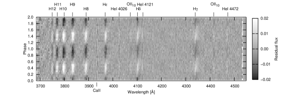
Figure 1.: Top: Line profile variations of the phase binned Steward data for the strongest mode $f1$ (period P=481.74 s). The Ca II line is of interstellar nature. Its variation is due to the stellar radial velocity correction. Besides the strong Balmer, He i and O ii lines are found to vary (from Tillich et al. 2007). Bottom: Variations of the temperature, log $g$ (both left), temperature and log $g$ residuals (both right) with best fit sine curve and statistical error bars.

As individual spectra are too noisy for a quantitative spectral analysis in terms of detecting very small variations, they were combined in an appropriate way. To be able to detect tiny variations for any pre-chosen pulsation mode, we determined the phase of each individual spectrum according to the selected pulsation period and co-added them weighted by S/N. To this end, a complete pulsation cycle was divided into twenty phase bins. In Fig. 1 (top), the phase dependent changes in the line profiles of the Steward data with respect to the mean spectrum are shown. It is evident that all the observed H, He i and O ii lines vary in the same way with phase. Effective temperatures ($T_{\rm{eff}}$), surface gravities ($\log{g}$), and helium abundances ($\log{n_{\mathrm{He}}/n_{\mathrm{H}}}$) were determined for every bin by fitting synthetic model spectra to all hydrogen and helium lines simultaneously, using a procedure developed by Napiwotzki et al. (1999). A grid of metal line-blanketed LTE model atmospheres with solar metal abundance was used.

We start our analysis with the dominant mode in radial velocity, which is expected to also show the largest variation in temperature and gravity (see Fig. 1, bottom). The variations of $T_{\rm{eff}}$ and $\log{g}$ are sinusoidal. Therefore, the pulsation semi-amplitude is determined by using a $\chi^{2}$ sine fitting procedure ($\Delta T_{\rm{eff}}=873.7\pm 16.5$ and $\Delta\log{g}=0.078\pm 0.003$). As expected the helium abundance remains constant. The first harmonic is clearly recovered in the temperature residuals (see Fig. 1 right, bottom). We then proceeded to search for and analyse weaker frequencies for which

Figure 2.: Variations of the temperature (left) and the log $g$ (right) for the four strongest frequencies after the cleaning procedure with the statistical error bars. The best fit sine curves are the full drawn lines. Note that the dominant mode is not perfectly eliminated. However the residuals are very small.

we developed a cleaning procedure. First we calculated synthetic spectra for every phase bin of the dominant pulsation frequency $f1$. Then they were summed up to create the mean synthetic spectrum for $f1$, which was subtracted from each phase bin spectrum to form the cleaning function. This correction was applied to all of the $\sim 9000$ individual spectra by subtracting the cleaning function for the corresponding phase of the dominant mode. All individual cleaned spectra were then summed into the appropriate phase bin for the corresponding periods of lower amplitude frequencies (from $f2$ onwards) and were analysed for the atmospheric parameter variations as described above. Results are summarized in Table 1 and plotted in Figs. 2 and 3. Unlike the isolated frequencies $f4$, $f2$ and $f3$ are too close together and therefore unresolved in our analysis. For the frequency $f9$, the errors of our data points ($\delta T_{\rm{eff}}=40\,\rm{K},\delta\log{g}=0.008\,\rm{dex}$) are of the same order of magnitude as the amplitude ($\Delta T_{\rm{eff}}=35\,\rm{K},\Delta\log{g}=0.003\,\rm{dex}$) and the detection of variations must be regarded as marginal. Nevertheless, this demonstrates that it is possible to reveal variations of atmospheric parameters of modes with radial velocity variations as small as $2\,\mathrm{km}\,\mathrm{s}^{-1}$. Frequencies $f5$ and $f6$ are isolated and therefore well resolved. By contrast frequencies $f7$, $f9$ and $f11$ are close together and therefore unresolved. While amplitude variations of atmospheric parameters are found for $f7$, the variations for $f9$ and $f11$ are below the detection limit. $f8$ and $f10$ are combination frequencies involving $f1$ ($f1$+$f5$ and $2\times f1$, respectively). For $f8$, the variation of $T_{\mathrm{eff}}$ is detected only marginally, whereas the gravity variation is pronounced (see Fig. 3 and Table 1). In order to characterise pulsation modes, it is also important to investigate the phase lags between temperature, gravity and radial velocity variations. These phase lags can be used to determine the deviations from an adiabatic change of condition. The radial velocities of individual spectra were taken from Paper I.

The amplitudes of their variations were determined in the same way as the temperature and gravity variations using the phase binning and cleaning technique described in Sect. 2. Phase lags between the variation of radial velocity and the atmospheric parameters can be derived directly by comparing the phases of their maxima. In order to determine the phase lags of the weaker modes, we used the temperature curves, and measured just the phase lags for two sine functions. As the formal fitting errors are unrealistically small, we use half the bin size ($\pm 0.025$) as error estimate. It is worth noting that for all recovered modes (except $f3$), the radial velocity variation reaches its maximum before the temperature variation. Furthermore, all the values of the phase lags lie around $0.25$($\widehat{=}\frac{\pi}{2}$) with small but significant deviations. This is the value we would expect for a completely adiabatic $p$-mode pulsation.

Table 1.: Semi-amplitudes of the temperature and gravity variations after cleaning for the four strongest modes derived from Steward data. Also the statistical error from the $\chi^{2}$ sine fitting is listed. Periods, frequencies and radial velocity amplitudes are taken from Paper I and therefore calculated for the whole MSST data run.

Name	Period	$f$	$v$	$\Delta T_{\rm{eff}}$	$\Delta\log{g}$
	[s]	[$\mu$Hz]	$[\mathrm{km}\,\mathrm{s}^{-1}]$	[K]	[dex]
				cleaning	cleaning
$f1$	481.74	2075.80	15.429	70.5$\pm$4.7	0.008$\pm$0.001
$f2$	475.61	2102.55	5.372	132.6$\pm$12.6	0.011$\pm$0.002
$f3$	475.76	2101.91	2.971	84.5$\pm$17.5	0.008$\pm$0.002
$f4$	364.56	2743.01	2.497	140.9$\pm$14.6	0.011$\pm$0.002
$f5$	503.55	1985.89	2.474	117.9$\pm$10.3	0.014$\pm$0.002
$f6$	528.71	1891.41	2.322	87.7$\pm$15.0	0.009$\pm$0.002
$f7$	361.86	2763.50	2.121	136.8$\pm$10.5	0.013$\pm$0.003
$f8$	246.20	4061.70	1.777	88.1$\pm$18.3	0.021$\pm$0.002

But as a real star is a non-adiabatic system due to its radiation of light, such deviations are to be expected. For the dominant mode $f1$, the phase lag between $T_{\rm{eff}}$ and $\log{g}$ is 0.3 (see Paper II) indicating that the temperature is highest shortly after the radius is smallest. After that, we consider the phase lags between the radial velocity and the gravity, which are supposed to have a strict relationship, as they are both produced by the movement of the stellar surface (i.e. the $g$ variation should be in line with the derivative of the radial velocity curve). Hence, we expect a phase lag of 0.25 between the RV curve and the $\log{g}$ curve. We apply the same fitting procedure as before. For the Steward data, most values seem to be in agreement with the theory within $\Delta\varphi=0.02$. This is consistent with our error estimate, except for frequencies $f3$, $f7$ and $f8$. The difficulties with $f3$ have already been discussed (see above) and the same may hold for $f7$ as it is also unresolved from $f9$, whereas frequency $f8$ is close to the detection limit (see above).

Figure 3.: Variations of the temperature (left) and the log $g$ (right) for the modes $f5$, $f6$, $f7$ and $f8$ after the cleaning procedure with sine fits and statistical error bars derived for the Steward data (from Paper II).

3. The Modelling of Pulsation Modes

For the modelling we used a routine, authored and introduced by Townsend (1997). The adiabatic code BRUCE has been developed to model non-radial pulsations for early-type main sequence stars. With a radiative shell and a convective core these stars have a similar structure as subdwarf B stars. Therefore the routines should also be able to describe the pulsations in these smaller sdB stars. In order to model the surface variations by a certain pulsation mode, the stellar parameters have to be known accurately, e.g. the polar values for radius, temperature, gravity and inclination as well as the equatorial rotation velocity. From these assumptions an equilibrium surface grid of the star, consisting of 51030 points, is calculated, taking into account any effects of the rotation on both surface geometry and surface temperature distribution. Thereafter this grid is perturbed by one (or several) well defined pulsation mode(s) to reveal the temporal propagation. The perturbation must be characterized through degree and order of a spherical harmonic and a perturbation velocity amplitude (for more details see Townsend 1997). The inclination angle plays a very important role for cancellation effects except for radial modes. BRUCE provides us with all the parameters neccessary for a spectral synthesis such as temperature, gravity and the projected values for velocity, surface area and surface normal for every point grid point on the stellar surface. The KYLE routine is based on a code authored by Falter (2001) and used to perform the spectral synthesis for every time step. For this purpose it interpolates in the same grid of LTE synthetic model spectra used for the spectral analysis (see Sect. 2) to obtain a spectrum for every point on the stellar surface. In order to shorten the calculation time, our model atmosphere grid was restricted to nine points, i.e. $30\,000$ K, $32\,500$ K and $35\,000$ K in temperature and $\log{g}$ of $5.0$, $5.25$ and $5.5$. The synthetic spectra cover $3\,000$ Å to $7\,000$ Å at a resolution of $0.1$ Å.

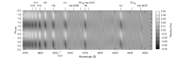
Figure 4.: Same as Fig. 1 but for the synthetic line profile variations derived from our slow rotating model i using the same procedures as for the observed data. Note that the first harmonic is clearly seen in both temperature and gravity at amplitudes similar to the observed ones (compare Fig. 1).

Falter (2001) used a simple wavelength independent limb darkening law in his code, which is the main drawback of this method according to Townsend (1997). So this approximation was regarded too crude and replaced by a quadratic law calculated for every wavelength of the synthetic spectra. Intensity spectra for nine angels were calculated from the model atmosphere and quadratic functions were fitted for every wavelength. The set of limb darkening coefficients was then input to KYLE. Fig. 4 (top) shows the theoretical line profile variation for a radial mode $l=0,m=0$ in PG1605$+$072 calculated with the BRUCE and KYLE code. We then used the same fitting procedure described in Sect. 2 to determine atmospheric parameters. To complete the set of stellar parameters we need to know the equatorial rotational velocity. Heber et al. (1999) determined the projected rotational velocity to $v_{\mathrm{rot}}\sin{i}\approx 39\,\mathrm{km}\,\mathrm{s}^{-1}$ from the observed spectral line broadening in a time integrated spectrum. However pulsational line broadening was not considered. As the RV amplitude of the dominant mode is large, it has to be corrected for. Taking into account the projection factor (Montanes–Rodriguez et al. 2001), we adopt a lower limit for the $v_{\mathrm{rot}}\sin{i}$ of about $17.4\,\mathrm{km}\,\mathrm{s}^{-1}$.
Based on these assumptions we tried two different models for PG1605+072: model i is a slowly rotating star with $i=90^{\circ}$ and $v_{\mathrm{rot}}=17.4\,\mathrm{km}\,\mathrm{s}^{-1}$, model ii is a fast rotating one with $i=7.7^{\circ}$ and $v_{\mathrm{rot}}=130\,\mathrm{km}\,\mathrm{s}^{-1}$. In the following section we compare the surface variations of these very different models.

Figure 5.: The modelled variations of the atmospheric parameter for the mode $l=1,m=+1$ (+) and $l=1,m=-1$ (x) with statistical error bars, sine fits and residuals for the slowly rotating model i (left) and the fast rotating model ii (right).

For the radial mode $l=0,m=0$ variations in $T_{\rm{eff}}$ and $\log{g}$ do not depend on inclination, due to the spherical symmetry of the problem. Also the residuals show variations of half the period attributed to the first harmonic, which have also been detected in the observational data at very similar amplitudes. This shows the reliability of our procedure. As can be seen from a comparison of Fig. 1 and Fig. 4, the predicted variations for $T_{\rm{eff}}$ are much larger than observed for the dominant mode, while that of the first harmonic are consistent with the observed ones. The predicted gravity variations however are consistent with observations for both the dominant and the first harmonic. In their analysis of Balloon 090100001 Østensen et al. (these proceedings) showed that the temperature variations may be strongly affected by non-adiabatic effects, while the gravity and velocity variations are not. If we therefore rely only on the gravity variations we could conclude that the dominant frequency is the radial mode.

For the $l=1,m=\pm 1$ modes in the slowly rotating model i we do not see a node line any more and therefore the pattern is similar to a weak radial mode again. But now as we change sign on $m$, the sinusoidal variation shifts with a factor of $0.5$ in phase (see Fig 5). The amplitudes in the slow rotating model for $l=1,m=+1$ are 1 714 K in $T_{\rm{eff}}$ and 0.057 in $\log{g}$, while for $l=1,m=-1$ they are 1 840 K in $T_{\rm{eff}}$ and 0.073 in $\log{g}$. Our result is that in a slowly rotating model the prograde and retrograde pulsation modes look quite the same, in terms of sinusoidal variation, except for a phase shift of $0.5$.

In the fast rotating model ii we view the star almost pole on, therefore we see the node line, which divides the star into 2 areas of different size. Either the hot part or the cold part of the star prevails and we obtain again a sinusoidal shape of the variations with a rather low amplitude. Our modelling shows that this is true only for the temperature variations. For $l=1,m=-1$ we measure amplitudes of 290 K in $T_{\rm{eff}}$ and 0.017 in $\log{g}$, while for $l=1,m=+1$ the variations are 175 K in $T_{\rm{eff}}$ and 0.001 in $\log{g}$. Hence, for a retrograde mode the gravity variation almost disappears, while for the prograde mode it does not. Applying this method we derived a complete set of amplitudes for the modes $l\leq 2$ (Tillich et al., in prep.).

References

- (1) Charpinet, S., Fontaine, G., Brassard D., et al. 1996, ApJ, 483, L123
- (2) Falter, S. 2001, Diploma Thesis, University of Erlangen–Nürnberg
- (3) Heber, U., Reid, I. N., Werner K., et al. 1999, A&A, 348, L25
- (4) Montañés Rodriguez, P., & Jeffery, C. S. 2001, A&A, 375, 411
- (5) Kilkenny, D., Koen, C., O’Donoghue, D., et al. 1999, MNRAS, 303, 525
- (6) Koen, C., O’Donoghue, D., Kilkenny, D., et al. 1998, MNRAS, 296, 317
- (7) Napiwotzki, R. 1999, A&A, 350, 101
- (8) Østensen, R., et al. 2007, these proceedings
- (9) O’Toole, S. J., Bedding, T. R., Kjeldsen, H., et al. 2000, ApJ, 537, L53
- (10) O’Toole, S. J., Heber, U., Jeffery, C. S., et al. 2005, A&A, 440, 667
- (11) Townsend, R. 1997, PhD Thesis, University College London
- (12) Tillich, A., Heber, U., O’Toole, S. J., et al. 2007, A&A, 473, 219
- (13) Tillich, A., et al. 2008, in prep.