Numerical studies of planar closed random walks.

Abstract

Lattice numerical simulations for planar closed random walks and their winding sectors are presented. The frontiers of the random walks and of their winding sectors have a Hausdorff dimension $d_{H}=4/3$. However, when properly defined by taking into account the inner 0-winding sectors, the frontiers of the random walks have a Hausdorff dimension $d_{H}\approx 1.77$.

Laboratoire de Physique Théorique et Modèles Statistiques. Université Paris-Sud, Bât. 100, F-91405 Orsay Cedex, France.

1 Introduction

Important progresses have been made in the past few years for the determination of critical exponents of planar Brownian curves based on a family of conformally invariant stochastic processes, the stochastic Loewner evolution (SLE) [1]. It has been proved [2] that the external frontier has a Hausdorff dimension $d_{H}=4/3$, a confirmation of a numerical conjecture by Mandelbrot [3]. The frontier of the Brownian curve is here defined as the set of points, i.e the part of the curve, where one stops when arriving from infinity and meeting it for the first time (the hull). This definition is geometrical, only the geometrical outer spreading of the curve does matter.

It is well known that random walks with $N$ steps approximate well planar Brownian curves of length $t$ when the number $N$ becomes large. The correspondance between $N$ and $t$ is $Na^{2}=2t$, where $a$ is the lattice spacing (it will be set to $1$ in the following). However, this statement has to be refined when winding properties are considered. For instance, the probability density of the angle $\Theta$ wound around the origin by an open Brownian curve is given, in the asymptotic regime, by Spitzer’s law [4] $\displaystyle P\left(x={2\Theta}/{\ln t}\right)={1}/({\pi}({1+x^{2}}))$. On the other hand, for a random walk on a two dimensional (2d) square lattice, the probability density is given by Belisle’s law [5] $\displaystyle P\left(x={2\Theta}/{\ln N}\right)={1}/({2}{\cosh(\pi x/2)})$. Note that all the moments are defined in the latter case whereas no moment exists in the former case, a fact which can be traced back to short-distance properties of Brownian motion, which are ignored when the lattice spacing is non zero.

In this paper, we adress numerically some properties of closed random walks on a 2d square lattice and discuss whether these results can also hold for Brownian curves. More precisely, we are concerned by fractal properties of the random walks and of their winding sectors.

For a closed Brownian curve of length $t$, a $n$-winding sector inside the curve is defined as a connected set of points that have been encircled $n$ times by the curve (more precisely $n$ is the number of anticlockwise minus clockwise encirclings).

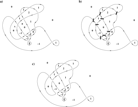
Figure 1: a) a closed curve with its winding sectors; b) the cuts required to open the fjord (see section 2); c) the closed curve with the fjord opened. a) and c) represent two possibe time histories of the same curve.

As an example, consider the curve of figure 1 a): leaving aside the infinite outside $(n=0)$-winding sector, which we call the ”sea”, this curve encloses five ($n=1$)-winding sectors, three ($n=-1$)-winding sectors, one ($n=2$)-winding sector, one ($n=-2$)-winding sector, and four $(n=0)$-winding sectors. Among them, three -marked as A, B and C- can be connected between themselves and to the outside ”sea” by simple cuts as indicated in figure 1 b). For this reason, they constitute what is called a ”fjord”. The last $0$-winding sector does not share this property, lying deep inside the curve. It is called a ”lake”.

Let us denote by $S_{n}$ the arithmetic area of all the $n$-winding sectors of a Brownian curve of length $t$, and by $S_{0}$ the arithmetic area of all the 0-winding sectors inside the curve, i.e. the fjords and lakes. Scaling properties for Brownian curves imply that the random variable $S_{n}$ scales like $t$. Its expectation value $<S_{n}>$ on the set of all closed curves of length $t$ has been computed by path integral methods [7]. As long as $n\neq 0$, $<S_{n}>={t}/{(2\pi n^{2})}$. On the other hand, when $n=0$, the 0-winding sectors arithmetic area diverges because, in this approach, the outside sea is necessarily taken into account. It was later shown by Werner in his thesis [8] that, for $n$ sufficiently large, $n^{2}S_{n}\to<n^{2}S_{n}>=t/(2\pi)$. Recently, using SLE methods [9], the expected value of the total arithmetic area $<S>=\sum_{n=-\infty}^{n=\infty}<S_{n}>$ of the curve has been obtained to be $<S>=t\pi/5$. It implies for the arithmetic area of the 0-winding sectors inside the curve $<S_{0}>=t\pi/30$, a rather striking result, bearing in mind that the lakes and fjords arithmetic areas were up to now out of reach, at least by methods inspired from physics.

Figure 2: a) a closed walk with its winding sectors; b) the same walk with an oriented frontier (the fjord is opened; see section 2); c) the two cuts needed to go from a) to b). a) and b) are two possible time histories of the same walk.

For closed random walks, the winding sectors can be defined in a similar way to those of Brownian curves: each elementary cell of the lattice is labelled by its winding number $n$; two adjacent cells with the same $n$ are connected if their commun edge is not spanned by the walker. A winding sector is a set of connected cells. For instance, the random walk in figure 2 a) encloses one (n=1)-sector, one (n=-1)-sector and a fjord constituted of the two $0$-winding sectors.

Figure 3: the average arithmetic area $<S_{n}>$ of all the $n$-winding sectors as a function of $n$; a) numerical simulations for random walks– the straight line is an exponential fit; b) the analytical result for Brownian curves.

In figure 3 a), the average arithmetic area $2<S_{n}>/N$ of all the $n$-winding sectors inside the random walk (log scale) is plotted as a function of the winding number $n\geq 0$, for 10000 closed random walks of $N=6000000$ steps. Clearly, the behavior is exponential as soon as $n\geq 3$. This is to be compared to the Brownian path integral result $<S_{n}>/t=1/(2\pi n^{2})$ (dashed curve in figure 3 b)). Moreover, for $n=0$, one obtains $2<S_{0}>/N\approx 0.13$ in place of the SLE result $<S_{0}>/t=\pi/30$ for Brownian curves.

In figure 4, on the other hand, the average total arithmetic area $2<S>/N$ is plotted as a function of the number of steps $N$, from $N=4000$ to $N=8000000$. It is manifest that as $N$ increases, $2<S>/N$ is closer and closer to the SLE result $<S>/t=\pi/5$ for Brownian curves. Thus, one concludes that the numerical lattice simulations for the $<S_{n}>$’s do not yield the Brownian path integral result $t/(2\pi n^{2})$, but their total sum correctly reproduces the SLE result.

Figure 4: the average arithmetic area enclosed by random walks as a function of the number of steps $N$; the $\pi/5$ horizontal line is the analytical result for Brownian curves.

This means that, quite generally and as expected, global properties of random walks do indeed hold for Brownian curves. A good agreement is also obtained for example while comparing the radii of gyration of random walks to those of Brownian curves, as we will see in Section 2. However, when details (for instance the properties of winding-sectors taken separately) are considered, the situation is less favorable. In that case, it is not a priori clear if and how numerical simulations on random walks give non ambiguous informations on Brownian curves, as already seen for Spitzer and Belisle’s laws.

2 Frontiers of closed random walks

Let us turn to the fractal properties of the external frontiers of random walks. When estimating the scaling and the Hausdorff dimension of the perimeter of its frontier, a characteristic length for the random walk is needed. A natural candidate is its radius of gyration, for which two definitions are possible. Consider first the successive positions $\overrightarrow{r_{i}},\;i=1,2,...,N,$ of the random walker and define the radius of gyration $r_{g}^{(1)}$ as

$$\left[r_{g}^{(1)}\right]^{2} = \frac{1}{N}\sum_{i=1}^{N}\left(\overrightarrow{r_{i}}-\overrightarrow{G}^{(1)}\right)^{2}$$ (1)

$$\overrightarrow{G}^{(1)} = \frac{1}{N}\sum_{i=1}^{N}\overrightarrow{r_{i}}$$ (2)

Alternatively, consider the part $\cal D$ of the plane enclosed by the random walk as an homogeneous solid of area $S$ and compute the radius of gyration $r_{g}^{(2)}$ of this solid

$$\left[r_{g}^{(2)}\right]^{2} = \frac{1}{S}\int\int_{\cal{D}}\left(\overrightarrow{r}-\overrightarrow{G}^{(2)}\right)^{2}\mbox{d}S$$ (3)

$$\overrightarrow{G}^{(2)} = \frac{1}{S}\int\int_{\cal{D}}\overrightarrow{r}\mbox{d}S$$ (4)

Figure 5: Comparison of the two definitions of the radius of gyration of closed random walks; the straight line is $<r_{g}^{(1)2}>=<r_{g}^{(2)2}>$.

Numerical simulations of $r_{g}^{(1)}$ and $r_{g}^{(2)}$ are presented in figure 5 ($N$ runs from $N=5000$ to $N=8000000$, the straight line is the diagonal). Clearly, both definitions lead to very close numerical estimates so that one can use indifferently the radius of gyration $r_{g}=(r_{g}^{(1)}\simeq r_{g}^{(2)})$ as a characteristic length for the random walk.

Incidentally, and as a further check of the correspondance between random walks and Brownian curves as far as their global characteristics are concerned, the average total arithmetic area $<S>$ as a function of $<r_{g}^{2}>$ is plotted in figure 6. The $r_{g}^{(1)}$ distribution, which has already been computed analytically for closed Brownian curves, again by means of path integral methods [10], gives $\displaystyle<\left(r_{g}^{(1)}\right)^{2}>={t}/{6}$. Using this input, one should get

$$<S>=\frac{\pi}{5}t=\frac{6\pi}{5}<r_{g}^{2}>\approx 3.77<r_{g}^{2}>$$ (5)

which is indeed the straight line plotted in figure 6.

Interestingly enough, (5) is related to random walks anisotropies- clearly, for an homogeneous isotrope disk, one should have $S=2\pi r_{g}^{2}$. The ratio ${\lambda_{+}}/{\lambda_{-}}$, where $\lambda_{+}>\lambda_{-}$ are the eigenvalues of the inertia tensor, can also be used to characterize the anisotropy. For closed Brownian curves, it has been known for some time [10] that

$$\frac{<\lambda_{+}>}{<\lambda_{-}>}\;=\;\frac{1+3\ln 2-\pi/2}{1-3\ln 2+\pi/2}\;\approx\;3.07$$ (6)

pointing to an elongated shape. We will come back to this point in Section 4.

Figure 6: the arithmetic area as a function of the square of the radius of gyration; the straight line is the fit $<S>=3.77<r_{g}^{2}>$.

Once the characteristic length $r_{g}$ of a random walk has been identified, one can turn to investigate the scaling of the perimeter of its external frontier with respect to this length. The external frontier is geometrically defined, accordingly to the external frontier of a Brownian curve, as the set of points, i.e. the part of the walk, obtained by arriving from infinity and stopping when one meets for the first time the walk. In figure 7 a), the scaling is displayed for closed random walks with a number of steps from $N=16000$ to $N=8000000$. The straight line shows that the external frontier scales like $\displaystyle r_{g}^{(4/3)}$ leading to the same Hausdorff dimension $d_{H}=4/3$ as the one obtained via SLE for Brownian curves. Therefore, as expected for a global characteristics, the scaling of the perimeter of the random walk correctly reproduces the Brownian curve Hausdorff dimension.

Figure 7: numerical results for the frontiers perimeters of closed random walks (the number of steps varying from $N=16000$ to $N=8000000$) as functions of the radius of gyration; a) external (geometric) frontier; b) external+fjords (oriented) frontier; c) external+fjords+lakes (disconnected) frontier; the slopes of the straight lines are : a) 4/3 , c) $1.77\approx 7/4$. See the text for b) (logarithmic corrections are included).

3 Oriented frontiers of closed random walks

Up to now, only the geometrical outer spreading of the random walks or of the Brownian curves has been taken into account to define their external frontiers. A consequence is that there is no way to span the frontiers defined in this way with a coherent orientation, as can be seen for example in figure 1 and figure 2. The impossibility to have a coherent orientation might incline to reconsider the definition of the frontiers. To this end, one should pay a particular attention to the possible time histories of a given random walk or Brownian curve.

A random walk on the lattice is nothing but a set of oriented edges spanned with Kirchoff conservation laws at the vertices. Consider first the random walk of figure 2. The two 0-winding sectors happen to be next to the outside sea. They constitute a fjord which can be opened to the outside by two simple cuts at particular intersections. In figure 2 a) and figure 2 b) are shown two possible time histories of the random walk (by convention when a random walk intersects itself at a later time it goes under its first trace). On the one hand, the time history of figure 2 a) is such that both the $0$-winding sectors are inside the walk (the fjord is closed) and its external frontier coincides indeed with its geometrical outer spreading (i.e. the part of the walk where one stops when arriving from infinity and meeting for the first time the walker). As already stressed, there is no coherent orientation on such a frontier. On the other hand, the time history of figure 2 b) is such that both the 0-winding sectors of the walk are now connected between themselves and to the sea (the fjord is opened). A frontier can then be defined by following the time history in figure 2 b) and, while doing so, by selecting the part of the walk which always has on one of its side the $0$-winding sector (the outside) and, necessarily, on the other side a ($n\neq 0$)-winding sector. It is manifest that this frontier is, by construction, spanned with a coherent orientation. Contrarily to the external geometrical frontier, it explores the inside of the walk while spanning the opened fjord. Rephrased in terms of cuts at intersections, the two cuts depicted in figure 2 c) are used to transform the walk of figure 2 a) into the walk of figure 2 b). Note that in this cutting process with an even number of cuts -here 2-, one has obtained a single random walk (it would not be the case if, for example, only one cut would have been used: two disconnected walks would then have been obtained).

Let us take advantage of what has been said but now for Brownian curves, for example the curve of figure 1. Consider the time history in figure 1 a): the external frontier is the geometrical one, as well as the frontiers of the $n$-winding sectors inside, which are all disconnected. The three 0-winding sectors which could be connected to the outside by simple cuts are inside the curve (closed fjord). However, eight cuts, as shown in figure 1 b), are sufficient to connect between themselves these 0-winding sectors and to open to the outside the fjord. Also, these cuts connect between themselves, when possible, the winding sectors of same winding number (here respectively the four $1$-winding sectors in the upper part of the path and the three $(-1)$-winding sectors in the lower part of the curve). One arrives at the Brownian curve of figure 1 c) whose frontier is obtained by following the time history in figure 1 c) and, while doing so, selecting the part of the curve which always has on one of its side the $0$-winding sector (the outside) and on the other side a ($\pm 1$)-winding sector. This frontier has, by construction, a coherent orientation. One also notes that the lake inside the $(-1)$-winding sector remains disconnected from the outside sea.

More generally, for any given Brownian curve, one can always find a time history with an oriented frontier consisting of the external + fjords frontier. Clearly, this oriented frontier is more intricate than the usual one since it does excursions inside the curve while spanning the opened fjords, which always happen to stretch from one side to another side of the curve.

One might wonder if these excursions around the fjords are sufficiently intricate to increase the Hausdorff dimension of the frontier, if such a dimension happens to exist. Numerical simulations in figure 7 b) indicate that the external+fjords (oriented) frontier perimeter scales like $\displaystyle r_{g}^{(4/3)}(\ln(r_{g}/8.5))^{0.205}$. Therefore, up to logarithmic corrections, the Hausdorff dimension is essentially unchanged and remains equal to $4/3$. However, when pushing further the logic of avoiding the $0$-winding sectors by also removing the lakes inside the random walks, i.e. when considering the external+fjords+lakes (disconnected) frontier, the numerics in figure 7 c) indicate a scaling with a Hausdorff dimension $d_{H}\approx 1.77\approx 7/4$. The increase of the dimension is nothing but an indication of the more and more intricate nature of the frontier, which goes not only around the fjords, but also deep inside the curve around the lakes (see figure 8 for an illustration of the distribution of fjords and lakes for a random walk of $N=1000000$ steps). Numerical simulations show that the ratio of the lakes average area to the fjords average area increases from $\approx 0.4$ to $\approx 1.9$ when $N$ goes from 15000 to 1000000, indicating that the lakes proliferate deep inside the walk when $N$ increases.

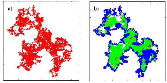
Figure 8: a) in red the closed random walk with $N=1000000$; b) in blue the fjords, in green the lakes. The fjords remain in general on the boundary of the walk, whereas the lakes proliferate deep inside the walk.

Both Hausdorff dimensions $4/3$ and $7/4$ are familiar in percolation [11]. A sketch of a site percolation cluster on a 2d lattice is given in figure 9 a) and numerical simulations for lattice sizes from 100$\times$100, 200$\times$200, …, up to 3200$\times$3200, are presented in figure 10.

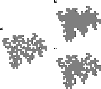
Figure 9: a) sketch of a site percolation cluster; b) its external frontier; c) its external+fjords frontier.

Figure 10: numerical results for site percolation ($p_{c}\approx 0.593$); the size of the 2d square lattice runs from 100$\times$100 to 3200$\times$3200; in correspondance with figure 9: b) the external frontier perimeter as a function of the cluster radius of gyration; c) the external+fjords frontier; a) the external+fjords+lakes frontier; the slopes of the fits are b) 4/3; c) 7/4; a) 1.9

On a 2d square lattice, at critical site percolation occupation $p_{c}\approx 0.593$, the external frontier (see figure 9 b)) of a percolation cluster, defined accordingly to the external frontier of random walks as arriving from infinity and stopping on the cluster, has a Hausdorff dimension $4/3$ (see figure 10 b)), as for random walks. In analogy with random walks, if one removes inside the percolation cluster the non percolating islands (see figure 9 c)) which can be connected to the outside by cuts at vertices (“fjords”), the Hausdorff dimension of the external+fjords frontier becomes $7/4$ (see figure 10 c)). If one also removes the non percolating islands deep inside the percolation cluster (“lakes”), one arrives at a disconnected percolation external+fjords+lakes frontier (see figure 9 a)) for which numerical simulations (see figure 10 a)) indicate a Hausdorff dimension $d_{H}\simeq 1.9>7/4$. Percolation and closed random walks happen to have only in commun the scaling dimension $4/3$ for their external frontier, the other dimensions being different ($7/4$ versus $4/3$, and $\simeq 1.9$ versus $\simeq 1.77$). It is however striking to note that in percolation the fjords are sufficiently intricate to increase the Hausdorff dimension of the perimeter, whereas there are not so for random walks.

4 Frontiers of winding sectors

A $n$-winding sector has been defined in section 1 as a set of connected cells of same winding $n$ inside a random walk (see figure 11).

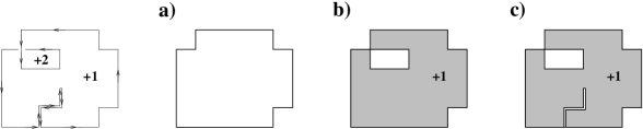
Figure 11: a (n=1)-winding sector; a) external (geometric) frontier; b) external+other windings frontier; c) external+other windings+ back-trackings frontier.

Numerical simulations for the $n=0,1,2,3$-winding sectors are presented in figure 12 and in figure 13 for $32000$ random walks of $N=4000000$ steps. For each walk, the radius of gyration, the enclosed arithmetic area, the anisotropy and the frontier are evaluated. Insufficient statistics makes it delicate to address larger $n$ which would require an increase of $N$ leading to rapidly prohibitive CPU times.

In figure 12, one considers, for each winding number, the set of all the corresponding winding sectors inside the random walks. The average value $S$ of the area enclosed by these winding sectors, plotted as a function of the square of their radius of gyration, leads to the scaling $S=3.77r_{g}^{2}$. This scaling is similar to the scaling of the arithmetic area of the random walks thenselves, plotted in figure 6.

Figure 12: the arithmetic area, $S$, enclosed by the $n$-winding sectors ($n=0,1,2,3$) as a function of their radius of gyration; the straight lines are the fits $S=3.77r_{g}^{2}$.

This result is somehow surprising since a winding sector by itself cannot be considered as a closed random walk. Nevertheless, anisotropy properties of the winding sectors do confirm this similarity between the random walks and their winding sectors. Numerical simulations for the ratio $\lambda_{+}/\lambda_{-}$ give for the $n=0$-winding sectors a value in the range 2.9-3.1 and for the $n=1,2,3$-winding sectors values in the range 2.9-3.2, which slightly increase with $n$. Again, these results are close to $<\lambda_{+}>/<\lambda_{-}>\approx 3.07$ of Section 2 for the random walks.

In figure 13, the scaling of the winding sector frontiers perimeters is considered. Let us first look at the perimeter of a winding sector external (geometric) frontier (see figure 11 a)). The scaling (straight line a)) is $r_{g}^{1.33}$, leading to a Hausdorff dimension $d_{H}\approx 4/3$ which is close to the dimension of the random walk frontiers.

Figure 13: numerical results for the frontiers perimeters of the $n$-winding sectors ($n=0,1,2,3$); a) external frontier; b) external+other windings frontier; c) external+other windings+back-trackings frontier; the slopes of the straight lines are a) 1.33 , b) 1.34 and c) 1.34 .

Now, a given winding sector can enclose other winding sectors: one can then define the frontier of the winding sector as its external frontier plus the frontiers of the enclosed sectors (see figure 11 b). This is the frontier seen from the inside of the $n$-winding sector and avoiding the cells belonging to the other sectors. The scaling (straight line b)) is $r_{g}^{1.34}$, which again leads to the Hausdorff dimension $d_{H}\approx 4/3$.

A random walk may also exhibit many back-trackings : one can define the frontier (see figure 11 c)) as the external frontier + the other windings + the edges inside the sector which have been spanned by the walker in both directions. The scaling (straight line c)) is still $r_{g}^{1.34}$, leading again to the dimension $d_{H}\approx 4/3$. It follows that whatever the definition of the frontier, the scaling is robust with a Hausdorff dimension remaining approximatively $d_{H}\approx 4/3$.

As a way of testing this robustness, one could relax a little the definition of a winding sector by considering that two adjacent cells belong to the same sector provided they have the same winding number, regardless if their common edges are spanned or not by the walker (see an example in figure 14).

Figure 14: The two ($n=1$)-winding sectors are considered as belonging to a unique sector.

For the scaling (with the square of the radius of gyration) of the average area enclosed by such winding sectors, the numerical simulations give a result similar to what was obtained previously. The same conclusion holds for the ratio $\lambda_{+}/\lambda_{-}$ which remains practically unchanged. Considering now the perimeter scalings, for the external frontier scaling the linear fit in figure 15 a) is $9.9\;r_{g}^{4/3}$ meaning that the Hausdorff dimension remains $d_{H}=4/3$. Now, for the external+other windings and external+other windings+back-trackings frontiers scalings in figure 15 b) and figure 15 c) respectively, linear fits with slopes slightly different from $4/3$ might be expected. However, a thorough analysis of the ratio of the frontiers perimeters yields the fits $10\;r_{g}^{4/3}(\ln r_{g})^{0.2}$ and $15.5\;r_{g}^{4/3}(\ln r_{g})^{0.2}$. It follows that, up to logarithmic corrections, the Hausdorff dimension remains again unaffected to the value $d_{H}\approx 4/3$.

Figure 15: numerical results for the frontiers perimeters of the $n$-winding sectors ($n=0,1,2,3$); a) external frontier; b) external+other windings frontier; c) external+other windings+back-trackings frontier; the slope of the straight line a) is 4/3. For b) and c), logarithmic corrections are included (see the text).

One concludes that the Hausdorff dimension of the winding sectors inside the random walk, is, as for the random walk itself, $d_{H}=4/3$.

5 Concluding remarks

Let us summarize the results obtained so far:

• we have discussed the correspondance between lattice random walk simulations and Brownian curves. The correspondance works well for global properties of the curves, as, for example, their radius of gyration, anisotropy and total arithmetic area. However, the arithmetic area of the $n$-winding sectors does not reproduce the path integral result for Brownian curves (eventhough, as already said, it does for their sum, i.e. the total arithmetic area).

• we have proposed a new definition for the frontier of a random walk and of a Brownian curve. It spans the $0$-winding sectors fjords connected to the sea. Contrary to the geometrical external frontier (the hull), this frontier has a coherent orientation.

• we have numerically established that, for the random walk, the Hausdorff dimension of both its external (geometric) frontier and its external+fjords (oriented) frontier (which does incursion inside the walk around the fjords) is, as for Brownian curves, $d_{H}=4/3$. On the other hand, the Hausdorff dimension of the external+fjords+lakes (disconnected) frontier is $d_{H}\approx 7/4$, which indicates that the $0$-winding lakes deep inside the walk contribute in a major way to the fractal properties of the frontier.

• we have numerically established that, for the random walk winding sectors, the Hausdorff dimension is robust at the value $d_{H}=4/3$. The scaling of the area of a winding sector with its radius of gyration is also very close to the scaling of the random walk itself.

Let us stress again that the scalings of the winding sectors are not obvious to interpret. Still one has found on a 2d square lattice strong numerical evidences which indicate some deep similarities between the random walks and their winding sectors -anisotropy, Hausdorff dimensions of the frontiers-, at least as far as the scalings are concerned. It would certainly be satisfying to understand more deeply these numerical results. Again, the similarity between the random walks and their winding sectors is especially puzzling.

The scaling dimension $4/3$ is known to be related via SLE to a conformal field theory with central charge $0$ (free fermions). For the scaling dimension $7/4$, the central charge is again $0$. However, the eventual link between those conformal models and closed random walks frontiers or winding sectors frontiers is far from obvious. Clearly, the $0$-winding sectors play an essential role for increasing the Hausdorff dimension of the closed random walk from $d_{H}=4/3$ to $d_{H}\approx 1.77$. On the other hand, we have seen in Section 1 that the $0$-winding sector arithmetic area $<S_{0}>$ is overestimated on the lattice. One can expect that the above question is related to a more fundamental one: what happens, in the continuum limit, i.e. for Brownian curves, to the winding sectors properties of random walks?

One of us (J.D.) acknowledges Thierry Jolicoeur for his help in vectorizing the programs. We thank Jesper Jacobsen for drawing our attention to the question of $n$-winding sector frontiers scaling and for his participation at the early stage of this work. We also thank Paul Wiegmann for interesting discussions.

References

- [1] G. F. Lawler, “Conformally invariant processes in the plane”, ICTP Lecture Notes 17 (2004) 305; W. Werner, arXiv: math.PR/0303354, “Random planar curves and Schramm-Loewner evolutions”, in Ecole d’été de Probabilités de Saint-Flour XXXII (2002), Springer Lecture Notes in Mathematics 1180 (2004) 113
- [2] W. Werner, arXiv: math.PR/0308164, “SLEs as boundaries of clusters of Brownian loops”; G. F. Lawler, O. Schramm and W. Werner, Mathematical Research Letters 8 (2001) 13
- [3] B.B. Mandelbrot (1982), The Fractal Geometry of Nature, Freeman
- [4] F. Spitzer, Trans. Am. Math. Soc. 87 (1958) 187
- [5] C. Belisle, Ann. Prob 17 (1989) 1377
- [6] J. Desbois, C. Furtlehner and S. Ouvry, Nucl. Phys.B 453 [FS] (1995) 759
- [7] A. Comtet, J. Desbois and S. Ouvry, J. Phys.A 23 (1990) 3563
- [8] W. Werner, Thèse, Université Paris 7 (1993) and Probability Theory and Related Fields (1994) 111
- [9] C. Garban and J. A. Trujillo Ferreras, arXiv:math.PR/0504496
- [10] G. Gaspari, J. Rudnick and A. Beldjenna, J. Phys. A 26 (1993) 1; F. Fougère and J. Desbois, J. Phys. A 26 (1993) 7253
- [11] B. Duplantier, arXiv: cond-mat/9901008