Fast rotating condensates in an asymmetric harmonic trap

Abstract

We investigate the effect of the anisotropy of a harmonic trap on the behaviour of a fast rotating Bose-Einstein condensate. Fast rotation is reached when the rotational velocity is close to the smallest trapping frequency, thereby deconfining the condensate in the corresponding direction. We characterize a regime of velocity and small anisotropy where the behaviour is similar to the isotropic case: a triangular Abrikosov lattice of vortices, with an inverted parabola profile. Nevertheless, at sufficiently large velocity, we find that the ground state does not display vortices in the bulk. We show that the coarse grained atomic density behaves like an inverted parabola with large radius in the deconfined direction, and keeps a fixed profile given by a Gaussian in the other direction. The description is made within the lowest Landau level set of states, but using distorted complex coordinates.

Vortices appear in many quantum systems such as superconductors and superfluid liquid helium. Rotating atomic gaseous Bose-Einstein condensates constitute a novel many body system where vortices have been observed Madison00 and various aspects of macroscopic quantum physics can be studied. In a harmonically trapped condensate rotating at a frequency close to the trap frequency, interesting features have emerged, presenting a strong analogy with quantum Hall physics. In the mean field regime, vortices form a triangular Abrikosov lattice Abr and the coarse grained density approaches an inverted parabola CKR ; WBP ; ABD . At very fast rotation, when the number of vortices becomes close to the number of atoms, the states are strongly correlated and the vortex lattice is expected to melt Cooper01 . In the mean field regime, Ho H observed that the low lying states in a symmetric 2D trap are analogous to those in the lowest Landau level (LLL) for a charged particle in a uniform magnetic field. This analogy allows a simplified description of the gas by the location of vortices: the wave function describing the condensate is a Gaussian multiplied by an analytic function of the complex variable $z=x+iy$. The zeroes of the analytic function are the location of the vortices. It is the distortion of the vortex lattice on the edges of the condensate which allows to create an inverted parabola profile CKR ; WBP ; ABD ; ABN2 for the coarse grained atomic density in the LLL.

The experimental achievement of rotating BEC involves anisotropic traps. An anisotropy of the trap can drastically change the picture in the fast rotation regime. In this case, the condensate becomes very elongated in one direction and forms a novel quantum fluid in a narrow channel. The investigation of the vortex pattern has been performed for an infinite strip which corresponds to the situation where the rotational frequency has reached the smallest trapping frequency gora ; palacios , and for an elongated condensate LNF ; oktel ; fetter07 . As pointed out by Fetter fetter07 , the description of the condensate can still be made in the framework of the lowest Landau level, defined by an anisotropic Gaussian, multiplied by an analytic function of $x+i\beta y$, where $\beta$ is related to the anisotropy of the trap and the rotational frequency. We are going to characterize a regime of fast rotation where there are no vortices in the bulk of the condensate and show that the coarse grained density profile is very different from the isotropic case: the behaviour is an inverted parabola with large expansion in the deconfined direction, while the extension remains fixed in the other direction, with a Gaussian profile.

We consider a 2D gas of $N$ atoms rotating at frequency $\Omega$ around the $z$ axis. The gas is confined in a harmonic potential, with frequencies $\omega_{x}=\omega\sqrt{1-\nu^{2}}$, $\omega_{y}=\omega\sqrt{1+\nu^{2}}$ along the $x,y$ axis respectively. The state of the gas is described by a macroscopic wave function $\psi$ normalized to unity, which minimizes the Gross-Pitaevskii energy functional. In the following, we choose $\omega$, $\hbar\omega$, and $\sqrt{\hbar/(m\omega)}$, as units of frequency, energy and length, respectively. The dimensionless coefficient $G=Na_{s}/a_{z}$ characterizes the strength of atomic interactions (here $a_{s}$ is the atom scattering length and $a_{z}$ the extension of the wave function in the $z$ direction for the initial 3-dimensional problem). The energy in the rotating frame is

$$E[\psi]=\int\left(\psi^{*}\left[H_{\Omega}\psi\right]+\frac{G}{2}|\psi|^{4}\right)\;dxdy$$ (1)

where $H_{\Omega}$ is defined by

$$H_{\Omega} = -\frac{1}{2}\nabla^{2}+\frac{1-\nu^{2}}{2}x^{2}+\frac{1+\nu^{2}}{2}y^{2}-\Omega L_{z}$$ (2)

and $L_{z}=i(y\partial_{x}-x\partial_{y})$ is the angular momentum. We are going to study the fast rotation regime where $\Omega^{2}$ approaches the critical velocity $\Omega_{c}^{2}:=1-\nu^{2}$ from below. Thus, we define the small parameter $\varepsilon$ by $\varepsilon^{2}=1-\nu^{2}-\Omega^{2}.$ The spectrum of the Hamiltonian (2) has a Landau level structure. The lowest Landau level is defined as (see fetter07 )

$$f(x+i\beta y)e^{\left[-\frac{\gamma}{8\beta}\left(x^{2}+(\beta y)^{2}\right)\right]-i\frac{\nu^{2}}{2\Omega}xy},\ f\text{ is analytic}$$ (3)

where $\gamma$ and $\beta$ are some constants related to $\Omega$ and $\nu$ given in the appendix; $\beta$ is close to 1 if $\nu$ is small. For such functions, $<{H_{\Omega}\psi},{\psi}>$ can be simplified (see the appendix and fetter07 ), and in the small $\varepsilon$ limit (with $\varepsilon\ll\nu$), we are left with the study of

$$E_{LLL}(\psi)=\int\frac{1}{2}\left(\varepsilon^{2}x^{2}+\kappa^{2}y^{2}\right)|\psi|^{2}+\frac{G}{2}|\psi|^{4}dxdy$$ (4)

where $\kappa^{2}\sim(\nu^{2}+\varepsilon^{2}/2)(2-\nu^{2})/(1-\nu^{2}).$ This energy only depends on the modulus of $\psi$. Hence, it is possible to forget the phase of $\psi$, and use a simplified definition of the LLL:

$$\psi(x,y)=f(x+i\beta y)e^{\left[-\frac{\gamma}{8\beta}\left(x^{2}+\beta^{2}y^{2}\right)\right]},\ f\text{ is analytic.}$$ (5)

We recall that the orthogonal projection of $L^{2}(\mathbb{R}^{2})$ onto the LLL is explicit B : $\Pi_{LLL}(\psi)=\frac{\gamma}{4\pi}\int e^{{-\frac{\gamma}{8\beta}\left(|z|^{2}-2z\overline{z^{\prime}}+|z^{\prime}|^{2}\right)}}\psi(x^{\prime},y^{\prime})dx^{\prime}dy^{\prime},$ where $z=x+i\beta y$ and $z^{\prime}=x^{\prime}+i\beta y^{\prime}$. We refer to the appendix of R for details on the operator $\Pi_{LLL}$, its kernel and the computations: if an LLL function $\psi$ (i.e $\psi$ satisfies (5)) is the ground state of (4), it is a solution of the projected Gross-Pitaevskii equation:

$$\Pi_{LLL}\left[\left(\frac{\varepsilon^{2}}{2}x^{2}+\frac{\kappa^{2}}{2}y^{2}+G|\psi|^{2}-\mu\right)\psi\right]=0,$$ (6)

where $\mu$ is the chemical potential.

The ground state of (4) without the analytic constraint is the inverted parabola

$$|\psi|^{2}=\rho_{\rm TF}:=\frac{2}{\pi R_{x}R_{y}}\left(1-\frac{x^{2}}{R_{x}^{2}}-\frac{y^{2}}{R_{y}^{2}}\right),$$ (7)

where $R_{x}=\left(\frac{4G\kappa}{\pi\varepsilon^{3}}\right)^{1/4}$, $R_{y}=\left(\frac{4G\varepsilon}{\pi\kappa^{3}}\right)^{1/4}.$ Note that in the isotropic case $\nu=0$ (that is $\kappa=\varepsilon$), one recovers the standard circular shape $R_{x}=R_{y}=[4G/(\pi\varepsilon^{2})]^{1/4}$. Since $\kappa\gg\varepsilon$, $R_{x}$ is always large. On the other hand, the behaviour of $R_{y}$ depends on the respective values of $\varepsilon$ and $\kappa\sim\nu\sqrt{2}$. We find that $R_{y}$ is large if $\nu\ll\varepsilon^{1/3}$ while $R_{y}$ shrinks if $\nu\gg\varepsilon^{1/3}$. We are going to see that in the first case, the profile (7) is reached in the fast rotation limit in the LLL using a vortex lattice, exactly as in the isotropic case, while in the second case, (7) is not a good description of the condensate because the properties of the LLL prevent $R_{y}$ from shrinking, and in particular the energy is much higher than that of (7).

In the first regime $\nu\ll\varepsilon^{1/3}$, which we call the weakly anisotropic case, figure 1 provides a typical vortex configuration, together with the corresponding density plot. It is obtained by minimizing the energy as a function of the location of vortices $z_{i}$ with a conjugate gradient method.

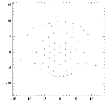
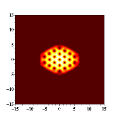
Figure 1: An example of (a): a configuration of the zeroes (b): density plot. There are 58 vortices with 23 visible vortices. $\nu=0.03,$ $\Omega=0.9985$, $\varepsilon^{2}=2\times 10^{-3}$, $G=3$.

The vortex lattice can be described as in the Abrikosov problem Abr ; H using the Theta function:

$$\phi(x,y;\tau)=e^{\frac{\gamma}{8\beta}\left({z^{2}}-{|z|^{2}}\right)}\Theta\left(\sqrt{\frac{\tau_{I}\gamma}{4\pi\beta}}z,\tau\right),$$ (8)

where $z=x+i\beta y$ and $\tau=\tau_{R}+i\tau_{I}$ is the lattice parameter. The zeroes of the function $\phi$ lie on the lattice $\sqrt{\frac{4\pi\beta}{\tau_{I}\gamma}}\left(\mathbb{Z}\oplus\mathbb{Z}\tau\right)$ and $|\phi|$ is periodic. The optimal lattice, that is the one minimizing $b(\tau)=\int|\phi|^{4}/(\int|\phi|^{2})^{2}$ is triangular, which corresponds to $\tau=e^{2i\pi/3}$ (the integrals are taken on one period). As in the isotropic case ABN2 , we can construct an approximate ground state of (4) by multiplying the solution (8) of the Abrikosov problem by a profile $\rho$ varying at the same scale as $\rho_{\rm TF}$ defined in (7). Since this product is not in the LLL, we project it onto the LLL and define $v=\Pi_{LLL}\left(\rho(x,y)\phi(x,y;\tau)\right)$ whose energy is

$$E_{\rm LLL}(v)=\int_{\mathbb{R}^{2}}\left(\frac{\varepsilon^{2}}{2}x^{2}+\frac{\kappa^{2}}{2}y^{2}\right)\rho+\frac{Gb(\tau)}{2}\rho^{2}dxdy,$$

up to an error of order $\sqrt{\kappa\varepsilon}(\kappa^{3}/\varepsilon)^{1/8}.$ Then, minimizing with respect to $\rho$ yields that $\rho(x,y)=\frac{1}{\sqrt{b(\tau)}}\rho_{\rm TF}\left(\frac{x}{b(\tau)^{1/4}},\frac{y}{b(\tau)^{1/4}}\right)$ where $\rho_{\rm TF}$ is given by (7). The condensate indeed expands in both directions, and a coarse-grained density profile is close to the anisotropic inverted parabola. The vortex lattice is not distorted by the anisotropy since $\beta$ is close to 1; it is still triangular, as displayed in figure 1. Nevertheless, as in the isotropic case ABD ; ABN2 , the lattice is distorted on the edges of the condensate, thereby allowing for a coarse-grained Thomas-Fermi profile in the LLL description.

However, when $\nu\gg\varepsilon^{1/3}$, that is for fast rotation, the behaviour is very different as illustrated in Figure 2: we are going to see that the ground state is close to a Gaussian in the $y$ direction multiplied by an inverted parabola in the $x$ direction. There is no vortex lattice. There are only invisible vortices whose role is to create the profile in the LLL. The function (7) does not provide the correct behaviour of the ground state: though $R_{y}$ in (7) is small, the condensate does not shrink in the $y$ direction but keeps a fixed Gaussian profilefoot2

$$g(x,y)=\left({\frac{\gamma\beta}{2\pi}}\right)^{1/4}\exp\left(-\frac{\gamma\beta}{4}y^{2}+i\frac{\gamma}{4}xy\right).$$ (9)

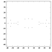
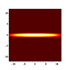
Figure 2: An example of (a): a configuration of the zeroes (b): density plot. There are only invisible vortices (32 vortices). Here, $\nu=0.73$ $\Omega=0.6820$, $\varepsilon^{2}=2\times 10^{-3}$, $G=3$. The extension in the $y$ direction is given by (9)

We are going to prove that if $u$ is the ground state and $p(x)$ its projection onto the Gaussian (9), then $p(x)$ is almost an inverted parabola. Indeed, in the LLL, we have the key identity $\int(\partial_{x}|\psi|)^{2}+(1/\beta^{2})(\partial_{y}|\psi|)^{2}=(\gamma/4\beta)\int|\psi|^{2}$ (see carlen ). By adding and subtracting $\kappa^{2}/(2\gamma\beta)\int|\psi|^{2}$ to the energy, and using this identity, we find

$$E_{LLL}(\psi)=-\frac{\kappa^{2}}{2\gamma\beta}+\int\left(\frac{2\kappa^{2}}{\gamma^{2}\beta^{2}}(\partial_{y}|\psi|)^{2}+\frac{\kappa^{2}}{2}y^{2}|\psi|^{2}\right)$$

$$+\int\left(\frac{2\kappa^{2}}{\gamma^{2}}(\partial_{x}|\psi|)^{2}+\frac{\varepsilon^{2}}{2}x^{2}|\psi|^{2}+\frac{G}{2}|\psi|^{4}\right).$$

This expression of the energy allows to analyze separately the contributions in the $x$ and $y$ directions. The ground state of $-(2/\gamma^{2}\beta^{2})\partial_{y}^{2}+(1/2)y^{2}$ is the modulus of (9) and the ground energy is $1/(\gamma\beta)$. Projecting any function of the LLL onto the space generated by (9) times a function of $x$, and using that $\varepsilon^{1/3}/\nu$ is small, we find that $E_{LLL}(u)\geq(\kappa^{2}/(2\gamma\beta))+E_{1D}(p(x))$ where

$$E_{1D}(p)=\int_{\mathbb{R}}\left(\frac{2\kappa^{2}}{\gamma^{2}}{(p^{\prime})}^{2}+\frac{1}{2}\varepsilon^{2}x^{2}p^{2}+\frac{G}{4}\sqrt{\frac{\gamma\beta}{\pi}}p^{4}\right)dx.$$ (10)

The minimizer of $E_{1D}$ among all $p$’s is of Thomas-Fermi type and we call it $q$:

$$q(x)=\sqrt{\frac{3}{4R}}\left(1-\frac{x^{2}}{R^{2}}\right)^{1/2}_{+}\ ,\quad R=\left(\frac{3G}{4\varepsilon^{2}}\sqrt{\frac{\gamma\beta}{\pi}}\right)^{1/3}$$ (11)

since $\varepsilon^{1/3}/\nu$ is small. This gives the energy estimate

$$\min E_{LLL}-\frac{\kappa^{2}}{2\gamma\beta}\geq E_{1D}(q)\sim\frac{3}{10}\left(\frac{3\varepsilon}{4}G\sqrt{\frac{\gamma\beta}{\pi}}\right)^{2/3}.$$ (12)

Let us point out that this lower bound is optimal since we can construct a test function in the LLL with this energy. We project a Dirac delta function in the $y$ direction times an inverted parabola in $x$, that is $v(x,y)=A\Pi_{LLL}[\delta_{0}(y)q(x)]$, where $q$ is the function (11):

$$v(x,y)=\frac{A\gamma}{4\pi}e^{-\frac{\gamma\beta}{8}y^{2}}\int_{\mathbb{R}}e^{-\frac{\gamma}{8\beta}\left((x-x^{\prime})^{2}-2ix^{\prime}\beta y\right)}q(x^{\prime})dx^{\prime}.$$ (13)

The constant $A=(2\pi/\gamma\beta)^{1/4}$ is a normalization factor. The fact that $q$ varies on a scale of order $\varepsilon^{-2/3}$ allows to expand (13) in powers of $\varepsilon^{2/3}$:

$$v(x,y)=\left(\frac{\gamma\beta}{2\pi}\right)^{1/4}q(x)\exp\left(-\frac{\gamma\beta}{4}y^{2}+i\frac{\gamma}{4}xy\right)\\ +\varepsilon^{2/3}\left(\frac{\gamma\beta}{2\pi}\right)^{1/4}q^{\prime}(x)iy\exp\left(-\frac{\gamma\beta}{4}y^{2}+i\frac{\gamma}{4}xy\right)$$ (14)

with an error of order $\varepsilon^{4/3}$. Inserting this expansion in the energy, we find

$$E_{\rm LLL}(v)=\frac{\kappa^{2}}{2\gamma\beta}+\int_{\mathbb{R}}\left(\frac{1}{2}\varepsilon^{2}x^{2}q(x)^{2}+\frac{G}{4}\sqrt{\frac{\gamma\beta}{\pi}}q(x)^{4}\right)dx$$ (15)

with an error of order $\varepsilon^{4/3}$. This matches our lower bound (12). Let us point out that according to (14), the wave function $v$ has no vortices in the bulk. This is corroborated by the numerical computation displayed in Figure 2. Nevertheless, the inverted parabola profile in the $x$ direction is obtained in the LLL thanks to the existence of invisible vortices, that is vortices outside the support of this parabola.

Let us point out that the operator $y^{2}$, whose ground state is the Gaussian (9) is bounded below by a positive constant in the LLL: $\int_{\mathbb{R}^{2}}y^{2}|\psi(x,y)|^{2}dxdy\geq\frac{1}{\gamma\beta}\int_{\mathbb{R}^{2}}|\psi|^{2}$. This can be viewed as a kind of uncertainty principle bound . This decoupling in the $x$ and $y$ directions is possible only when the leading order term in the energy $\kappa^{2}/(\gamma\beta)\sim\nu^{2}$, is larger than the energy of (7) $\sqrt{G\nu\varepsilon}$, that is when the ratio $\nu^{3}/\varepsilon$ is large. When $\nu^{3}/\varepsilon$ becomes of order 1, all the terms in the energy seem of the same order, the decoupling in the $x$ and $y$ variables is no longer meaningful, and (7) does not provide the good behaviour either. The analysis in this intermediate regime is still open: it could display rows of vortices as obtained by palacios .

The estimate of the energy (12) allows us to justify the validity of the model: indeed, the mean field approximation is valid if the number $N$ of particles is much larger than the number of one-particle states allowed by the chemical potential $\mu$, that is $N\gg\mu/\mu_{1}$. Thanks to (12) and (16), we find $N\gg G^{2/3}/\epsilon^{1/3}\nu$. Since $G$ is of order 1, $\epsilon^{2}\sim 10^{-3}$ and $\nu\leq 10^{-1}$, this criterion is satisfied as long as $N$ is greater than $10^{4}$, which corresponds to actual values in experiments. However, if $\varepsilon$ gets too small, this condition gets violated and the states get correlated. The LLL approximation is valid if the 1D energy $E_{1D}$ is much smaller than the gap $\mu_{2}$ between the LLL and the first excited state: $(G\varepsilon)^{2/3}\ll 1$.

Conclusion: When the anisotropy is small compared to how close the rotational velocity is to the critical velocity, that is $\varepsilon^{1/3}\gg\nu$, the behaviour is similar to the isotropic case with a triangular vortex lattice. A striking new feature is the non-existence of visible vortices for the ground state of the energy in the fast rotation regime, that is when $\varepsilon^{1/3}\ll\nu$. The profile of the ground state is a large inverted parabola in the deconfined direction and a fixed Gaussian in the other direction. Our analysis indicates that an asymmetric rotating condensate undergoes a similar transition as a condensate placed in a quadratic+quartic trap where at large rotation the bulk of the condensate does not display vorticesJFS . Our investigation opens new prospects for the experiments: in particular, if a condensate at rest is set to sufficiently large rotation, then vortices should not be nucleated.

Appendix

As computed in fetter07 on the basis of ideas of Valatin valatin , the eigenvalues of the Hamiltonian $H_{\Omega}$ are $1,\mu_{1}^{2},1,\mu_{2}^{2}$, where $\mu_{1}^{2}=1+\Omega^{2}-\sqrt{\nu^{4}+4\Omega^{2}},$ $\mu_{2}^{2}=1+\Omega^{2}+\sqrt{\nu^{4}+4\Omega^{2}}.$ We define $\alpha=\sqrt{\nu^{4}+4\Omega^{2}},$ $\beta_{1}=({2\Omega\mu_{1}})/({\alpha-2\Omega^{2}+\nu^{2}}),$ $\beta=\beta_{2}=({2\Omega\mu_{2}})/({\alpha+2\Omega^{2}+\nu^{2}}),$ $\gamma=({2\alpha})/{\Omega},$ $\lambda_{1}^{2}=({\alpha-2\Omega^{2}+\nu^{2}})/({2\alpha}),$ $\lambda_{2}^{2}=({\alpha+2\Omega^{2}+\nu^{2}})/{2\alpha},$ $d=({\gamma\lambda_{1}\lambda_{2}})/{2},$ $c=({\lambda_{1}^{2}+\lambda_{2}^{2}})/{2\lambda_{1}\lambda_{2}}.$ Then $H_{\Omega}=\frac{1}{2}\left(a_{1}^{\dagger}a_{1}+a_{1}a_{1}^{\dagger}\right)+\frac{1}{2}\left(a_{2}^{\dagger}a_{2}+a_{2}a_{2}^{\dagger}\right)$ where $a_{2}=\frac{\mu_{2}}{\sqrt{2}}\left(-i\lambda_{1}d^{-1}\partial_{x}+c\lambda_{1}y\right)+\frac{i}{\sqrt{2}}\left(-i\lambda_{2}\partial_{y}-\left(d\lambda_{1}^{-1}-\lambda_{2}cd\right)x\right)$, and $a_{1}=\frac{\mu_{1}}{\sqrt{2}}\left(-i\lambda_{2}d^{-1}\partial_{y}+c\lambda_{2}x\right)+\frac{i}{\sqrt{2}}\left((\lambda_{1}cd-d\lambda_{2}^{-1})y-i\lambda_{1}\partial_{x}\right).$ We have: $\left[a_{2},a_{2}^{\dagger}\right]={\mu_{2}},\quad\left[a_{1},a_{1}^{\dagger}\right]={\mu_{1}},$ and all other commutators vanish. The LLL is defined by $a_{2}\psi=0,$ that is $f(x+i\beta_{2}y)e^{\left[-\frac{1}{8\beta_{2}}\left(\frac{2\alpha-\nu^{2}}{\Omega}x^{2}+\frac{2\alpha+\nu^{2}}{\Omega}(\beta_{2}y)^{2}\right)\right]-i\frac{\nu^{2}}{4\Omega}xy}$, with $f$ analytic. It is always possible to change the analytic function $f(\xi)$ into $f(\xi)\exp(-\delta\xi^{2})$ in the above definition, since $\exp(-\delta\xi^{2})$ is an analytic function of $\xi$. Hence, for $\delta=\nu^{2}/(8\Omega\beta_{2}),$ we find the alternative definition of the LLL (3), with $\beta=\beta_{2}$. This definition is equivalent to the one given by Fetter in fetter07 . However, contrary to fetter07 , the coefficients in (3) are not singular in the limit $\varepsilon\to 0.$ Indeed, in this limit, $\beta_{2}\sim\sqrt{(1-\nu^{2})/(1-\nu^{2}/2)}$ and $\gamma\sim(4-2\nu^{2})/\sqrt{1-\nu^{2}}$. This is due to the addition of the above-mentionned complex Gaussian in the definition of the LLL. In the LLL, we have $\left\langle H_{\Omega}\psi,\psi\right\rangle=\frac{1}{2}\left\langle\left(a_{1}^{\dagger}a_{1}+a_{1}a_{1}^{\dagger}\right)\psi,\psi\right\rangle+\frac{\mu_{2}}{2}\left\langle\psi,\psi\right\rangle.$ We then express $x$ and $y$ as linear combinations of $a_{1},a_{2},a_{1}^{\dagger},a_{2}^{\dagger}$ fetter07 ; oktel and get, if $\psi\in LLL$,

$$\left\langle H_{\Omega}\psi,\psi\right\rangle=\frac{\mu_{2}}{2}-\frac{\mu_{1}}{4}\left(\beta_{1}\beta_{2}+\frac{1}{\beta_{1}\beta_{2}}\right)\\ +\frac{\gamma}{4}\int\left(\mu_{1}\beta_{1}x^{2}+\frac{\mu_{1}}{\beta_{1}}y^{2}\right)|\psi|^{2}dxdy$$ (16)

which provides (4) with $\kappa^{2}=\gamma\mu_{1}/2\beta_{1}$ since $\gamma\mu_{1}\beta_{1}\sim 2\varepsilon^{2}$. Note that $\mu_{1}\sim\nu\varepsilon$ and $\mu_{2}\sim(2-\nu^{2})$.

Acknowledgements. We would like to thank A.L.Fetter and J.Dalibard for very useful comments. We also acknowledge support from the French ministry grant ANR-BLAN-0238, VoLQuan and express our gratitude to our colleagues participating to this project, in particular Th.Jolicœur and S.Ouvry.

References

(1)
K. W. Madison, F.Chevy, W.Wohleben, J.Dalibard, Phys. Rev. Lett.
84, 806, (2000);
J.R. Abo-Shaeer, C. Raman, J.M Vogels, and W. Ketterle, Science
292, 476 (2001);
P.C. Haljan, I. Coddington, P. Engels, E.A. Cornell, Phys. Rev.
Lett. 87, 210403 (2001).
(2) A.A. Abrikosov, Zh. Eksp. Teor. Fiz. 32, 1442
(1952). W. H. Kleiner, L. M. Roth and S. H. Autler, Phys. Rev. 133, A1226, (1964).
(3)
N.R. Cooper, N.K. Wilkin, and J.M.F. Gunn, Phys. Rev. Lett.
87, 120405 (2001).
(4)
T. L.Ho Phys. Rev. Lett. 87 060403 (2001).
(5)
G. Watanabe, G. Baym and C. J. Pethick, Phys. Rev. Lett.
93, 190401 (2004).
(6)
N. R. Cooper, S. Komineas and N. Read, Phys. Rev. A 70,
033604 (2004).
(7) A. Aftalion, X. Blanc, J. Dalibard, Phys. Rev. A 71,
023611 (2005).
(8) A. Aftalion, X. Blanc, F. Nier, Phys. Rev. A 73,
011601(R) (2006).
(9) E. A. Carlen, J. Funct. Analysis 97, 231
(1991). The proof is based on an explicit formula for the gradient
of a holomorphic function : , which allows to obtain that
satisfies .
(10) S. Sinha and G. V. Shlyapnikov, Phys. Rev. Lett. 94,
150401 (2005).
(11) P. Sánchez-Lotero and J. J. Palacios, Phys. Rev. A
72, 043613 (2005).
(12) M. Linn, M. Niemeyer, and A. L. Fetter, Phys. Rev. A 64, 023602 (2001).
(13) M. Ö. Oktel, Phys. Rev. A 69, 023618 (2004)
(14) Alexander L. Fetter, Phys. Rev. A 75, 013620
(2007).
(15) V. Bargmann Comm. Pure Appl. Math. 14, 187-214 (1961).
(16) N.Read Phys.Rev. B 58 (1998) 16262.
(17)This Gaussian is both
a solution to and for some constants .
(18) If , and , then our uncertainty principle implies a bound
on , which means that an function cannot shrink in the
direction.
(19) A. L. Fetter, B. Jackson, and S. Stringari, Phys. Rev. A 71, 013605 (2005).
(20) J. G. Valatin, Proc. Roy. Soc. 238, 132 (1956).