Temperature dependence of the slip length in polymer melts at attractive surfaces
Abstract
Using Couette and Poiseuille flow, we extract the temperature dependence of the slip length, , from molecular dynamics simulations of a coarse-grained polymer model in contact with an attractive, corrugated surface. is dictated by the ratio of bulk viscosity and surface mobility. At weakly attractive surfaces, a lubrication layer forms, is large and increases upon cooling. Close to the glass transition temperature, , very large slip lengths are observed. At a more attractive surface, a“sticky surface layer” is build up, which gives rise to a small slip length. Upon cooling, decreases at high temperatures, passes through a minimum and grows upon approaching . At strongly attractive surfaces, the Navier-slip condition fails to describe Couette and Poiseuille flow simultaneously. The simulation results are corroborated by a schematic, two-layer model suggesting that the observations do not depend on the details of the computational model.
Rapid miniaturization of microfluidic devices has led to new questions in hydrodynamics Squires and Quake (2005) which often involve the role of boundaries. The microscopic structure at the solid-fluid interface dictates wettability and friction and much effort has been directed towards tailoring these properties. The effect of microscopic surface properties can be incorporated into a continuum description via a boundary condition (HBC) to the Navier-Stokes equation. Theoretical and experimental studies of fluid flow in confined systems have demonstrated that the no-slip boundary condition, which postulates that the tangential velocity at the surface vanishes, can be violated Tropea et al. (2007) and the fluid slips past the surface. In the context of microfluidics, slip is often preferred because it reduces the amount of shear stress or pressure drop required to maintain flow. Hence, higher through-put can be generated in microfluidic devices. The amount of slip can be quantified by the slip length, . The slip boundary condition was formulated by Navier in 1823 as a balance between viscous stress and friction stress at the surface:
| (1) |
where denotes the friction coefficient and the bulk viscosity of the liquid. characterizes the position at which the hydrodynamic boundary condition is to be applied. Both parameters, and , characterize the HBC. The value of the slip length, , has been measured experimentally for a variety of systems and the results have attracted abiding interest Tropea et al. (2007). Typically, the scale of the slip length in simple liquids is set by the size of the constituents of the fluid Joly et al. (2006). There are, however, notable exceptions: For instance, topographically structured surfaces have been designed to generate large slip, nano-bubbles or the formation of a lubrication layer at the solid-fluid interface due to surface segregation of a low-molecular weight component in a polydisperse melt can increase the slip length. Recently, a careful analysis of the rim profile of dewetting polymer films has also provided evidence of slip length of the order of micrometers, which is significantly larger than microscopic length scales in the system Fetzer et al. (2006).
In this Letter, we investigate the impact of surface interactions and the concomitant effective viscosity Goel et al. (2008) at the surface on the HBC by molecular dynamics simulations of a standard, coarse-grained polymer model Grest and Kremer (1986). We show that (i) the stronger is the attraction between fluid particles and substrate the smaller is the slip length, (ii) slip lengths can grow large as the glass transition temperature of the fluid is approached, and (iii) for strongly attractive surfaces the Navier slip condition (1) fails to provide a HBC that simultaneously describes Poiseuille and Couette flow. Our simulation results are corroborated by a phenomenological two-layer model.
In our model, polymers are comprised of coarse-grained segments that interact via a truncated and shifted Lennard-Jones potential with cut-off, . Length and energy scales are set by the parameters and of the potential. Neighboring segments are bonded together by a FENE (Finitely Extensible Non-linear Elastic) potential Grest and Kremer (1986). The model exhibits a glass transition temperature and the dynamics in the bulk and in confinement has been recently reviewed Baschnagel and Varnik (2005). A Dissipative Particle Dynamics (DPD) thermostat is used to control temperature, . The solid surface is modeled by two rigid layers of Lennard-Jones interaction centers arranged on a FCC lattice Servantie and Müller (2008). By varying the strength, , of the Lennard-Jones potential between solid and fluid, we tune the adhesion and slip.
In order to mimic experimental conditions, the simulations are performed at the coexistence pressure where the polymer melt coexists with a vapor of vanishingly low density. Rather than using a constant pressure algorithm we tune the distance, , between the walls to attain the coexistence density. The system size is chosen large enough for the properties in the center of the film to be independent from the strength of the solid-fluid interaction. Periodic boundaries are applied in both, and directions and the dimensions of the simulation cell are and , respectively. At low temperature the fluid consists of 20 000 coarse-grained segments and the distance between the walls varies between and . At higher temperature , when the effect of the substrate propagates not that far into the film, we use 10 000 particles, and varies between and .
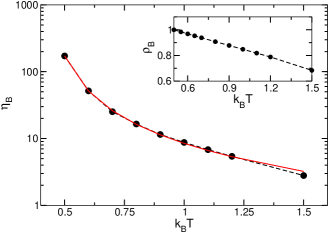
As a first result, we depict in Fig. 1 the temperature dependence of the bulk viscosity extracted from the velocity profile, , of Poiseuille flow at the center of the film. The steady-state Navier-Stokes equation yields
| (2) |
where , , and denote the number density of the liquid, the bulk viscosity, and the volume force applied to the segments, respectively. The inset represents the liquid density, , at coexistence. Upon reducing temperature, the model exhibits a glass transition at . The bulk viscosity above the glass transition temperature, , is well describable by the power law, predicted by Mode Coupling theory Götze and Sjögren (1992). Fitting the simulation data in Fig. 1 yields and , which agrees with previous studies Bennemann et al. (1998).
Due to pronounced layering effects at the solid surface, the effective, near-surface viscosity, , deviates from the bulk behavior. While viscosity is only properly defined in the bulk, there are several ways to estimate an effective local viscosity. One consists in computing the local shear stress and defining as the ratio between the local shear stress and the velocity gradient. However, the gradient of the velocity profile is difficult to extract with sufficient accuracy and in previous studies an explicit form of the velocity profile has been assumed Varnik and Binder (2002). Here, we instead analyze the local mobility of the fluid. Assuming that the mobility can be estimated by the Einstein relation , we obtain the estimate 111For the motion of a coarse-grained segment in a viscous fluid the Einstein formula relates the self-diffusion coefficient to the viscosity of the surrounding fluid. For short chain lengths and low temperatures close to , the fluid viscosity is dominated by non-bonded interactions and chain connectivity is less important. In fact, the Einstein relation describes the bulk behavior surprisingly well..

The local diffusivity is obtained from the mean square displacement parallel to the surfaces as where only particles that remain in region for the entire time of the calculation contribution to the average Harmandaris et al. (2005). We have computed the local diffusivity at temperature for . The boundaries for the bulk region are chosen such that the bulk properties are independent of the substrate strength. The fluid properties gradually change as a function of the distance from the solid-liquid interface. Our choice of the width of the boundary region is a compromise: It is wide enough such that segments remain sufficiently long in the boundary region to determine the diffusivity, and it is narrow enough in order for the properties to be dominated by surface effects. As we decrease , the near-surface mobility becomes larger as shown in Fig. 2 and the average time a particle stays in the surface region decreases. In the bulk region, the diffusivity is independent from the solid-fluid attraction, . In the inset, we depict the ratio and observe that substrate strengths larger than approximately result in a ratio , i.e., a “sticky surface layer” is formed. For , the surface mobility is enhanced and a lubrication layer forms at the solid-fluid interface.
In order to measure the slip length, , and position, , of the HBC, we simultaneously compute Couette and Poiseuille flow profiles Müller and Pastorino (2008); Servantie and Müller (2008) for the different solid-fluid interaction strengths as a function of temperature. The shear rate employed is small enough such that does not depend on the strength of the flow Priezjev and Troian (2004). To simulate planar shear flow (Couette) the surfaces are moved at constant velocity, . We typically employed where denotes the reduced Lennard-Jones time unit. Poiseuille flow is generated by applying a force, on all particles. In our simulations, the volume force varies between . Complementary information is obtained by calculating the friction coefficient, , from equilibrium molecular dynamics by integrating the transverse force auto-correlation function Bocquet and Barrat (1994). Previous studies for our model have shown that this procedure gives rise to consistent results at high temperatures Servantie and Müller (2008).
The velocity in the bulk region at the center of the film, , are fitted by linear or parabolic profiles as predicted by macroscopic hydrodynamics for Couette and Poiseuille flow. Let and denote the positions, where these linear and parabolic profiles extrapolate to vanishing velocity, then the slip length and the position of the hydrodynamic boundary condition are given by:
| (3) |
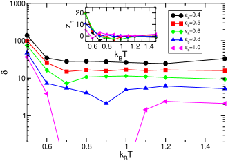
The results for the slip length are depicted in Fig. 3 and the distance to the wall of the hydrodynamic boundary in the inset. We see that the temperature dependence of is highly sensitive to temperature and solid-fluid interaction. First, we observe that independently from the slip length diverges as we approach the glass transition temperature, , because the fluid eventually behaves like a solid. Already at , i.e., about above the glass transition temperature of our model, has increased by an order of magnitude compared to the approximately constant value at high temperature. This observation offers an explanation for the surprisingly large slip length observed in the dewetting experiment of Fetzer et al. Fetzer et al. (2006), which were performed in the vicinity of the glass transition temperature.
The results for the position, , of the HBC do not vary significantly with the strength of the fluid-solid interaction over the entire temperature regime. At high temperature, the position is close to the top of the solid surface, while it gradually shifts inwards as the temperature is reduced towards . This effect goes along with a growing distance over which the liquid structure is altered by the surface as can be observed from the pronounced packing effects in the density profile.
While the position, , does not significantly depend on , the behavior of the slip length qualitatively changes with the strength of the solid-fluid interaction. While the values of corresponding to and decrease monotonously with , we observe a non-monotonous variation of the slip length for larger attraction, . For very strong attraction, , there is even a region of intermediate temperatures where and thus Eq. (3) has no solution. This marks the failure of the Navier slip condition to parameterize the near-surface flow solely by the material properties of the solid surface.
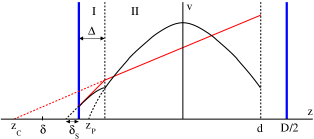
In order to rationalize these simulation results and explore whether they are universal or specific to our coarse-grained polymer model, we propose a schematic two-layer model depicted in Fig. 4. Within this model, we approximate the gradual variation of the fluid properties as a function of the distance from the solid surface by a boundary region of width, , which is characterized by a surface viscosity, , and the bulk with viscosity, . Within each layer, the fluid is described by the Navier-Stokes equation. At the interface between the solid surface and the boundary layer, we impose a Navier slip condition (1) with a microscopic slip length, . At the interface between the surface layer and bulk, we require the continuity of shear stress and velocity,
| (4) |
For planar shear flow one obtains for the linear velocity profile in the central bulk region
| (5) |
where quantifies the shear stress. If a volume force is applied to the fluid, one obtains a parabolic velocity profile in the boundary layer and in the bulk. Using Eq. (2) and the boundary conditions (1) and (4), we obtain for the latter:
| (6) |
Finally, Eq. (3) yields the slip length
| (7) |
The first term describes the effect of the surface layer, the second term arises from the microscopic slip at the solid surface. For surfaces with a large surface mobility, , a lubrication layer is formed and results in an enhanced slip length, , compared to the microscopic slip at the solid-fluid interface. On the other hand, if the solid-fluid interactions give rise to a boundary layer with large effective viscosity, , the presence of this sticky layer at the substrate reduces the slip length, ). Moreover, if
| (8) |
the velocity far away from the surface cannot be described by the Navier-Stokes equation and a Navier slip boundary condition (1).
This schematic model can rationalize the observations in our molecular dynamics simulation: (i) At high temperature, kinetic effects will dominate the behavior, thus . In this case, is equal to the microscopic slip length . (ii) Upon cooling the fluid, the bulk viscosity increases. If the solid-fluid interactions are weak, , a lubrication layer is formed and the slip length increases, . (iii) If the coupling between solid and fluid is strong, however, the ratio decreases upon cooling and so does . If the ratio becomes sufficiently small (see Eq. (8)), as it does in the case for our model, the Navier slip condition fails. Upon approaching from above, however, the slip length passes through a minimum and increases. The latter effect stems from the temperature dependence of the microscopic slip length, , which diverges for .
In conclusion, surface interactions can modify the near-surface mobility and thus can be exploited to control the hydrodynamic boundary condition. Very large slip lengths can be expected in the vicinity of the glass transition of the fluid. Depending on the strength of the interaction between the solid surface and the fluid, slippage may be enhanced or reduced, and at strongly attractive surfaces the Navier slip condition may even fail to provide an appropriate boundary condition to the Navier-Stokes equation with parameters that solely depend on the surface material. These findings of the simulations are corroborated by a schematic two-layer model which shows that the effects are universal and are not a consequence of the non-Newtonian nature of the polymer liquid employed in our study.
We thank K. Ch. Daoulas, K. Jacobs, R. Seemann, C. Pastorino, and B. Wagner for stimulating discussions. Financial support was provided by the DFG priority program “nano- and microfluidics” under grant Mu 1674/3. We gratefully acknowledge computer time at the Jülich Supercomputer Center.
References
- Squires and Quake (2005) T. M. Squires and S. R. Quake, Rev. Mod. Phys. 77, 977 (2005).
- Tropea et al. (2007) C. Tropea, A. Yarin, and J. F. Foss, Handbook of Experimental Fluid Mechanics (Springer, New York, 2007).
- Joly et al. (2006) L. Joly, C. Ybert, and L. Bocquet, Phys. Rev. Lett. 96, 046101 (2006).
- Fetzer et al. (2006) R. Fetzer, M. Rauscher, A. Münch, B. A. Wagner, and K. Jacobs, Europhys. Lett. 75, 638 (2006).
- Goel et al. (2008) G. Goel, W. P. Krekelberg, J. R. Errington, and T. M. Truskett, Phys. Rev. Lett. 100, 106001 (2008).
- Grest and Kremer (1986) G. S. Grest and K. Kremer, Phys. Rev. A 33, 3628 (1986).
- Baschnagel and Varnik (2005) J. Baschnagel and F. Varnik, J. Phys. Cond. Matt. 17, R851 (2005).
- Servantie and Müller (2008) J. Servantie and M. Müller, J. Chem. Phys. 128, 014709 (2008).
- Götze and Sjögren (1992) W. Götze and L. Sjögren, Rep. Prog. Phys. 55, 241 (1992).
- Bennemann et al. (1998) C. Bennemann, W. Paul, K. Binder, and B. Dünweg, Phys. Rev. E 57, 843 (1998).
- Varnik and Binder (2002) F. Varnik and K. Binder, J. Chem. Phys. 117, 6336 (2002).
- Harmandaris et al. (2005) V. A. Harmandaris, K. C. Daoulas, and V. G. Mavrantzas, Macromolecules 38, 5796 (2005).
- Müller and Pastorino (2008) M. Müller and C. Pastorino, Europhys. Lett. 81, 28002 (2008).
- Priezjev and Troian (2004) N. V. Priezjev and S. M. Troian, Phys. Rev. Lett. 92, 018302 (2004).
- Bocquet and Barrat (1994) L. Bocquet and J.-L. Barrat, Phys. Rev. E 49, 3079 (1994).