EFFECT OF DISTANCE ERRORS: APPLICATIONS TO SDSS EARLY-TYPE GALAXIES

Noisy distance estimates associated with photometric rather than spectroscopic redshifts lead to a mis-estimate of the luminosities, and produce a correlated mis-estimate of the sizes. We consider a sample of early-type galaxies from the SDSS DR6 and apply the generalization of the $V_{max}$ method to correct for these biases. We show that our technique recovers the true redshift, magnitude and size distributions, as well as the true size-luminosity relation. Regardless the specific application outlined here, our method impacts a broader range of studies, when at least one distance-dependent quantity is involved.

1 Introduction and significance

Galaxy scaling relations play a crucial rule in constraining galaxy formation models. However, a bias will be intrinsically present in these correlations if the transformation from observable to physical quantity involves one or more distance-dependent observables, due to noise in the distance estimate. Distances are only known approximately if photometric redshifts are available but spectroscopic redshifts are not. This is already the case of many current surveys (e.g. SDSS, Combo-17, MUSYC, Cosmos), where the number of objects with photometric redshifts is more than an order of magnitude bigger than that of spectroscopic redshifts, and will be increasingly true of the next generations of deep multicolor photometric surveys (e.g. DES, LSST, SNAP).

Therefore, methods for recovering unbiased estimates of distance-dependent observables, and of the joint distribution of luminosity, color, size, from magnitude limited photometric redshift datasets are indeed necessary (Rossi & Sheth 2007 $\!{}^{{\bf?}}$; Sheth 2007 $\!{}^{{\bf?}}$; Lima et al. 2008 $\!{}^{{\bf?}}$). In what follows, we show the essential inversion character of this class of problems by using a selected sample of early-type galaxies from the SDSS DR6 – for which both photo-zs and spectro-zs are known – and by applying our deconvolution techniques to reconstruct the true distributions and the scaling relations.

2 The SDSS early-type sample

The catalog we use is based on the Sloan Digital Sky Survey (SDSS) Data Release 6, available online through the Catalog Archive Server Jobs System (CasJobs). We adopt selection criteria suitable to early-type galaxies. Specifically, from the DR6 galaxy photometric sample (PhotoObjAll in the Galaxy view), and from the spectroscopic sample (SpecObjAll), we select objects according to these general criteria:

• Petrosian magnitudes in the range $14.50\leq m\leq 17.45$ for the r band;

• Concentration index $r_{petro,90}/r_{petro,50}>2.5$ in the $i$ band;

• Likelihood of the de Vaucouleur’s model $>0.8$;

• Objects with both photometric and spectroscopic redshifts available.

No redshift or velocity dispersion cuts were made. Our catalog contains $163,718$ objects, and consists of model magnitudes, petrosian radii, De Vaucouleurs and exponential fit scale radii along with their corresponding axis ratios in the $r$ band, photometric redshifts and photo-z errors. We do not apply any K-corrections to our de-reddened model magnitudes, since our main goal is to test the deconvolution technique rather than characterize the exact relations. We select photometric redshifts from the SDSS $Photoz$ Table. This set of photometric redshifts has been obtained with the template fitting method, which simply compares the expected colors of a galaxy with those observed for an individual galaxy (Budavári et al. 2000 $\!{}^{{\bf?}}$). The spectroscopic pipeline assigns instead a final redshift to each object spectrum by choosing the emission or cross-correlation redshift with the highest CL. In the selection of our sample, we tried to minimize the use of spectral information, but more robust constraints can be applied in order to reduce errors in galaxy classification.

3 Essence of the deconvolution problem

If we indicate with $\zeta$ and $z$ the photometric and spectroscopic redshifts, respectively, the problem of estimating the intrinsic redshift distribution $N(z)$ – normalized number of objects which lie at redshift $z$ – is best thought of as a deconvolution problem, and if $p(\zeta|z)$ is the probability of estimating the redshift as $\zeta$ when the true value is $z$, then the distribution of estimated redshifts is:

$${\cal N}(\zeta)=\int N(z)~{}p(\zeta|z)~{}{\rm d}z.$$ (1)

Equation (1) is an integral equation of the first kind of the Fredholm type, with the conditional probability $p(\zeta|z)$ as kernel. A simple iterative scheme proposed by Lucy (1974) $\!{}^{{\bf?}}$ allows one to reconstruct the intrinsic distribution after a few iterations, provided a suitable first guess.

Similarily, let $M$ denote the true absolute magnitude and $\mathcal{M}$ that estimated using $\zeta$ rather than $z$. Use $D_{\rm L}(z)$ to denote the luminosity distance, and $\phi(M)$ to indicate the number density of galaxies with absolute magnitudes $M$. Let $V_{\rm max}$ denote the largest comoving volume out of which an object of absolute magnitude $M$ can be seen, and $V_{\rm min}$ the analogous if the catalog is also limited at the lower end. The (true) number of galaxies with absolute magnitude $M$ for a magnitude limited catalog is:

$$N(M)=\phi(M)[V_{\rm max}(M)-V_{\rm min}(M)],$$ (2)

and the total number of objects with estimated absolute magnitudes $\cal M$ is:

$${\cal N}(\cal M) = \int{\rm d}M~{}\phi(M)~{}\Theta[V_{\rm max}(M),V_{\rm min}(M),M,{\cal M}]$$

$$= \int{\rm d}M~{}N(M)~{}\frac{\Theta[V_{\rm max}(M),V_{\rm min}(M),M,{\cal M}]}{[V_{\rm max}(M)-V_{\rm min}(M)]},$$

where

$$\Theta(V_{\rm max},V_{\rm min},M,{\cal M})=\int_{D_{\rm L}(V_{\rm min})}^{D_{\rm L}(V_{\rm max})}{\rm d}D_{\rm L}~{}\frac{{\rm d}V_{\rm com}}{{\rm d}D_{\rm L}}~{}p(M-{\cal M}|M,D_{\rm L}).$$ (4)

Note that since $V_{\rm max}$ and $V_{\rm min}$ are known functions of $M$, $\Theta$ itself is just a complicated function of $M$ and ${\cal M}$. Dividing (4) by $[V_{\rm max}(M)-V_{\rm min}(M)]$ yields:

$$\frac{\Theta(M,{\cal M})}{[V_{\rm max}(M)-V_{\rm min}(M)]} = \int{\rm d}D_{\rm L}~{}\frac{{\rm d}V_{\rm com}/{\rm d}D_{\rm L}}{[V_{\rm max}-V_{\rm min}]}~{}p(M-{\cal M}|M,D_{\rm L})$$ (5)

$$= \int{\rm d}D_{\rm L}~{}p(D_{\rm L})~{}p(M-{\cal M}|M,D_{\rm L})$$

$$= \int{\rm d}D_{\rm L}~{}p(D_{\rm L})~{}p({\cal M}|M,D_{\rm L})$$

$$\equiv p({\cal M}|M).$$

Therefore, the observed magnitude distribution can be expressed as a simple one-dimensional deconvolution, namely:

$${\cal N}({\cal M})=\int N(M)~{}p({\cal M}|M)~{}{\rm d}M.$$ (6)

Along the same lines, use $R$ to denote $\log_{\rm 10}$ of the physical size, and $\cal R$ to denote the estimated size based on the photometric redshift $\zeta$. Then it is readily shown that one can also think of ${\cal N}({\cal R})$ as being a convolution of the true number of objects with size $R$,

$${\cal N}({\cal R})=\int{\rm d}R~{}N(R)~{}p({\cal R}|R).$$ (7)

Direct measurements of the conditional probabilities allow one to reconstruct the intrinsic distributions from the observed ones, using a simple one-dimensional deconvolution. Similarily, a two-dimensional extension of the previous formalism is necessary if scaling relations are reconstructed from photometric data (Rossi & Sheth 2007) $\!{}^{{\bf?}}$.

Figure 1: [Left] Observed, intrinsic and reconstructed redshift distributions for the SDSS DR6 early-type sample. The dotted histogram was used as a starting guess for the one-dimensional deconvolution algorithm. Convergence is achieved after a few iterations. [Center] Reconstruction of the intrinsic $N(M)$ distribution from the distribution of estimated redshifts. Dotted histogram shows the observed absolute magnitude distribution, used as a starting guess. Jagged line is the reconstructed intrinsic distribution, after $10$ iterations. [Right] Reconstruction of the intrinsic $N(R)$ distribution from the distribution of estimated redshifts. Dotted histogram shows the observed size distribution, used as a starting guess. Jagged lines show the reconstructed intrinsic distribution after $8$ iterations.

4 Redshift, magnitude and size distributions. Scaling relations

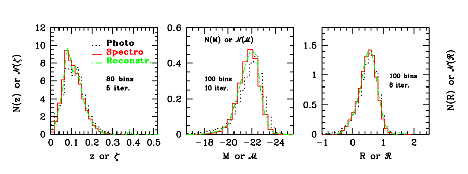
Results of applying our deconvolution techniques to the observed redshift, magnitude and size distributions are shown in Figure 1. Specifically, the left panel shows the photometric or observed redshift distribution (dotted line), the spectroscopic or intrinsic distribution (solid line) and its reconstruction after a few iterations (jagged line), based on the Lucy (1974) $\!{}^{{\bf?}}$ inversion algorithm. The $p(\zeta|z)$ distributions are inferred directly from the SDSS data, and in our deconvolution code (DeFaST) we use splines to interpolate for these conditional distributions. In the same fashion, by measuring the conditional probabilities $p({\cal M}|M)$ and $p({\cal R}|R)$ directly from the catalog, it is possible to apply the one-dimensional deconvolution algorithm to reconstruct the magnitude and size distributions (equations 6 and 7). The central panel shows the reconstruction (jagged line) of the intrinsic distribution of absolute magnitudes (solid histogram) after $10$ iterations. The observed distribution of $\cal M$ (dotted line) was used as a convenient starting guess in the deconvolution algorithm. Similarily, the right panel shows the one-dimensional reconstruction (jagged line) of the size distribution. The intrinsic distribution of physical sizes (solid line) is recovered after a few iterations, when the observed distribution of $\cal R$ (dotted line) is used as a convenient starting guess.

Figure 2: Effect of photo-$z$ on the size-luminosity correlation in our SDSS early-type catalog. In the left panel, contours and solid line show the ${\cal R}-{\cal M}$ relation associated with photo-$z$s, whereas the right panel shows the intrinsic $R-M$ relation measured from spectro-zs. Note the bias (shallower slope in panel on left) which results from the fact that the photo-$z$ distance error moves points down and left or up and right on this plot. Squares in left panel show the binned starting guess for the 2d deconvolution algorithm, triangles in right panel show the result after 7 iterations. Circles are the expected binned intrinsic relation, obtained from spectroscopic information.

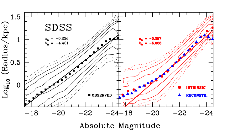
Although the difference between the intrinsic and observed size distributions is remarkably small, this departure suffices to bias the size-luminosity relation – as presented in Figure 2. In fact, photometric redshift errors broaden both the magnitude and size distributions, but changes to the estimated absolute magnitudes and sizes are clearly not independent. These correlated changes have a significant effect on the size-luminosity relation, even when the brodening of one of the two distributions is not severe. In our SDSS catalog $\langle{\cal R}|{\cal M}\rangle\propto-0.226$, whereas $\langle R|M\rangle\propto-0.257$. In Figure 2 it is shown that the use of photo-$z$ introduces a bias in the size-luminosity relation (shallower slope in panel on left). Squares in left panel show the binned starting guess for the two-dimensional deconvolution algorithm, triangles in right panel show the result after $7$ iterations and circles are the expected binned intrinsic relation, obtained from spectroscopic information. Convergence to the true solution is clearly seen.

5 Summary

Using a selected sample of early-type galaxies from the SDSS DR6, for which both photo-zs and spectro-zs are known, we applied our one- and two-dimensional deconvolution techniques (Sheth 2007 $\!{}^{{\bf?}}$; Rossi & Sheth 2007 $\!{}^{{\bf?}}$) to reconstruct the unbiased redshift, magnitude and size distributions, as well as the magnitude-size relation. We showed that our technique recovers all the true distributions and the joint relation, to a good degree of accuracy. We argued that the problem of reconstructing the true magnitude or size distribution is best thought as a one-dimensional deconvolution problem, and provided little algebra to show that this is indeed possible. We showed that even if the distribution of physical sizes is almost unbiased, a bias in the magnitude distribution sufficies to compromise the size-luminosity relation in an important way. We used our 2D technique to correct for this effect.

Although the discussion was phrased mainly in terms of the luminosity-size relation, the methods developed here are quite general and can be applied to recover any intrinsic correlations between distance-dependent quantities (even for $n$-correlated variables). Potentially, they impact a broader range of studies when at least one distance-dependent quantity is involved.

References

- [1] Rossi, G., & Sheth, R. K. 2007, ArXiv e-prints, 710, arXiv:0710.1165
- [2] Sheth, R. K. 2007, MNRAS, 378, 709
- [3] Lima, M., Cunha, C. E., Oyaizu, H., Frieman, J., Lin, H., & Sheldon, E. S. 2008, ArXiv e-prints, 801, arXiv:0801.3822
- [4] Budavári, T., Szalay, A. S., Connolly, A. J., Csabai, I., & Dickinson, M. 2000, AJ, 120, 1588
- [5] Lucy L. B., 1974, AJ, 79, 745