Pion condensation of quark matter in the static Einstein universe

Abstract

In the framework of an extended Nambu–Jona-Lasinio model we are studying pion condensation in quark matter with an asymmetric isospin composition in a gravitational field of the static Einstein universe at finite temperature and chemical potential. This particular choice of the gravitational field configuration enables us to investigate phase transitions of the system with exact consideration of the role of this field in the formation of quark and pion condensates and to point out its influence on the phase portraits. We demonstrate the effect of oscillations of the thermodynamic quantities as functions of the curvature and also refer to a certain similarity between the behavior of these quantities as functions of curvature and finite temperature. Finally, the role of quantum fluctuations for spontaneous symmetry breaking in the case of a finite volume of the universe is shortly discussed.

I Introduction

Low-energy nonperturbative effects in quantum chromodynamics (QCD), especially at nonzero densities, can only be studied by approximate methods within the framework of various effective models. It is well known that light meson physics is described by four-fermion models, such as the Nambu–Jona-Lasinio (NJL) model, which was successfully used to deal with dynamical chiral symmetry breaking (D$\chi$SB) both in the vacuum and in hot/dense baryonic matter (see, e.g. [1] ; [2] , as well as the reviews volkov ; hatsuda and references therein). Recently, much attention has been paid to the effects of diquark condensation and color superconductivity (CSC). The first studies of the gap equations and the Ginzburg-Landau free energy for a system of relativistic fermions led to the conclusion that superconductive and color superconductive states may arise in baryonic matter [9] ; [10] (see also the recent papers alford ; bekvy ). Another interesting phenomenon, the condensation of charged pions, which may appear in dense hadronic matter due to an asymmetry of its isospin composition, has been investigated in the framework of QCD-like effective models, including the NJL model, as well son ; [15] ; [23] ; 23 ; [18] ; [17] ; [19] .

Note that all these phenomena might be inherent to physics of compact stars, where rather strong magnetic as well as gravitational fields are present. Therefore, investigations of the influence of an external (chromo-)magnetic field on the properties of the D$\chi$SB phase transition oscil ; [3] , color superconductivity 3 and pion condensation [21] effects are quite appropriate. In particular, it was shown in oscil ; [3] ; 3 ; [21] that external fields significantly change the properties of the chiral and CSC phase transitions. In several papers, in the framework of the NJL model, the influence of a gravitational field on the D$\chi$SB due to the creation of a finite quark condensate $\langle\bar{q}q\rangle$ has been investigated at zero values of temperature and chemical potential MUTA ; Elizalde ; Elizalde_Shilnov ; Gorbar . The study of the combined influence of curvature and temperature has been performed in Inagaki_Ishikawa . Recently, the dynamical chiral symmetry breaking and its restoration for a uniformly accelerated observer due to the thermalization effect of acceleration was studied in ohsaku2 at zero chemical potential. Further investigations of the influence of the Unruh temperature on the phase transitions in dense quark matter with a finite chemical potential, and especially on the restoration of the broken color symmetry in CSC were made in qqrindler .

One of the widely used methods of accounting for gravitation is based on the expansion of the fermion propagator in powers of small curvature $R$ Bunch_Parker ; Parker_Toms . For instance, in kim_klim , the three-dimensional Gross-Neveu model in a spacetime with a weakly curved two-dimensional surface was investigated, using an effective potential at finite curvature and nonzero chemical potential. In paper Goyal_Dahiya , this weak curvature expansion was used in considering the D$\chi$SB at non-vanishing temperature and chemical potential. It should, however, be mentioned that near the phase transition point, one cannot consider the critical curvature $R_{c}$ to be small and therefore the weak curvature expansion method can not be applied. Hence, in the region near the critical regime different nonperturbative methods or exact solutions with finite values of $R$ should be used. This kind of solution with consideration for the chemical potential and temperature in the gravitational background of a static Einstein universe has been considered in Huang_Hao_Zhuang . There it was demonstrated that chiral symmetry is restored at large values of the space curvature. Analogous studies of diquark condensation and the related color symmetry breaking under the influence of a gravitational field have been performed recently in the model of a static Einstein Universe in etz . Recall that this model is widely discussed in literature either as a solution of the Einstein equations with a given cosmological constant and a nonvanishing energy-momentum tensor of an ideal fluid as a source, or as an initial state in inflationary cosmology with a scalar field, and the cosmological constant as its vacuum energy (see, for instance, ellis ). Moreover, the Einstein universe and other suitably generalized compact curved spacetimes were extensively employed for studying the phenomenon of Bose-Einstein condensation (see, e.g. smith and references therein). As is well known, one of the possible models for the expanding universe is the closed Friedmann model. Since the formation of quark condensates is expected to take place considerably faster than the expansion rate of the Universe, its radius can be considered in our calculations as constant. In this sense, the chosen model of a static Einstein universe can be considered as a simple cosmological model for a space with positive curvature. On the other hand, the same form of the metric does also hold for the interior of a (collapsing) spherically symmetric star, thereby admitting also a non-cosmological interpretation of the chosen model.

As was mentioned above, in quark matter there may arise another remarkable phenomenon, pion condensation. Up to now little information about the properties of pion condensation in the presence of external fields has been obtained. In particular, there arises the interesting question, what influence gravitational fields can produce on pion condensation. The main aim of the present paper is just to give a detailed investigation of this issue.

In order to be able to consider the effects of gravitation on pion condensation in a rigorous nonperturbative way, we will investigate here the phase structure of isotopically asymmetric quark matter in the framework of an extended NJL model with dynamical breaking of chiral and flavor symmetries in the static Einstein universe. In particular, our calculations are performed in the most simple case, restricting ourselves, for simplicity, to the flavor $SU(2)$ group. By using the mean field approximation, we will then derive an analytical expression for the thermodynamic potential of the NJL model that will enable us to calculate the chiral and pion condensates of quarks moving in a space with constant positive curvature. On this basis, we study, in particular, the phase portraits of the model. Our paper is organized as follows. Section II, III contain the Nambu-Jona-Lasinio model in curved spacetime and the general formalism for the derivation of the thermodynamical potential. Numerical calculations and conclusions are given in sections IV, V. Finally, some estimates of the role of quantum fluctuations in the case of a closed universe are given in the appendix.

II Nambu – Jona-Lasinio model in curved spacetime

Suppose that dense, isotopically asymmetric quark matter (in this case the densities of $u$ and $d$ quarks are different) in curved spacetime is described by an extended NJL model with the following action:

$$S=\int d^{4}x\sqrt{-g}~{}{\mathcal{L}}_{q},$$ (1)

and the Lagrangian

$${\mathcal{L}}_{q}=\bar{q}\Big{[}i\gamma^{\nu}\nabla_{\nu}-m+\mu\gamma^{0}+\delta\mu\tau_{3}\gamma^{0}\Big{]}q+G\Big{[}(\bar{q}q)^{2}+(\bar{q}i\gamma^{5}\vec{\tau}q)^{2}\Big{]},$$ (2)

where the quark field $q(x)\equiv q_{i\alpha}(x)$ is a flavor doublet ($i=1,2$ or $i=u,d$) and color triplet ($\alpha=1,2,3$) as well as a four-component Dirac spinor (the summation in (2) over flavor, color and spinor indices is implied); $\tau_{i}$ ($i=1,2,3$) are Pauli matrices. In 4-dimensional curved spacetime with signature $(+,-,-,-)$, the line element is written as

$$ds^{2}=\eta_{\hat{a}\hat{b}}e_{\mu}^{\hat{a}}e_{\nu}^{\hat{b}}dx^{\mu}dx^{\nu}.$$

The gamma-matrices $\gamma_{\mu}$, the metric $g_{\mu\nu}$ and the vierbein $e^{\mu}_{\hat{a}}$, as well as the definitions of the spinor covariant derivative $\nabla_{\nu}$ and spin connection $\omega^{\hat{a}\hat{b}}_{\nu}$ are given by the following relations Parker_Toms :

$$\{\gamma_{\mu}(x),\gamma_{\nu}(x)\}=2g_{\mu\nu}(x),\quad\{\gamma_{\hat{a}},\gamma_{\hat{b}}\}=2\eta_{\hat{a}\hat{b}},\quad\eta_{\hat{a}\hat{b}}={\rm diag}(1,-1,-1,-1),$$

$$g_{\mu\nu}g^{\nu\rho}=\delta^{\rho}_{\mu},\quad g^{\mu\nu}(x)=e^{\mu}_{\hat{a}}(x)e^{\nu\hat{a}}(x),\quad\gamma_{\mu}(x)=e^{\hat{a}}_{\mu}(x)\gamma_{\hat{a}}.$$ (3)

$$\nabla_{\mu}=\partial_{\mu}+\Gamma_{\mu},\quad\Gamma_{\mu}=\frac{1}{2}\ \omega^{\hat{a}\hat{b}}_{\mu}\sigma_{\hat{a}\hat{b}},\quad\sigma_{\hat{a}\hat{b}}=\frac{{1}}{4}[\gamma_{\hat{a}},\gamma_{\hat{b}}],$$

$$\omega^{\hat{a}\hat{b}}_{\mu}=\frac{1}{2}e^{\hat{a}\lambda}e^{\hat{b}\rho}[C_{\lambda\rho\mu}-C_{\rho\lambda\mu}-C_{\mu\lambda\rho}],\quad C_{\lambda\rho\mu}=e^{\hat{a}}_{\lambda}\partial_{[\rho}e_{\mu]\hat{a}}.$$ (4)

Here, the index $\hat{a}$ refers to the flat tangent space defined by the vierbein at spacetime point $x$, and the $\gamma^{\hat{a}}(\hat{a}=0,1,2,3)$ are the usual Dirac gamma-matrices of Minkowski spacetime. Moreover $\gamma_{5}$, is defined, as usual (see, e.g., Parker_Toms ), i.e. to be the same as in flat spacetime and thus independent of spacetime variables.

In order to describe the quark composition of matter we introduced $\mu=\mu_{B}/3$ in (2) as the quark number chemical potential. Since the generator $I_{3}$ of the third component of isospin is equal to $\tau_{3}/2$, the quantity $\delta\mu$ in (2) is half the isospin chemical potential, $\delta\mu=\mu_{I}/2$. If the bare quark mass $m$ is equal to zero, then at $\delta\mu=0$, apart from the trivial color SU($3$) symmetry, the Lagrangian (2) is invariant under the chiral group $SU_{L}(2)\times SU_{R}(2)$ transformations. However, at $\delta\mu\neq 0$ this symmetry is reduced to the subgroup $U_{I_{3}L}(1)\times U_{I_{3}R}(1)$ (here and above the subscripts $L,R$ imply that the corresponding group acts only on the left, right handed spinors, respectively). It is convenient to present this symmetry as $U_{I_{3}}(1)\times U_{AI_{3}}(1)$, where $U_{I_{3}}(1)$ and $U_{AI_{3}}(1)$ are the isospin and axial isospin subgroup of the chiral $SU_{L}(2)\times SU_{R}(2)$ group. Quarks are tranformed under these subgroups in the following way

$$U_{I_{3}}(1):~{}~{}~{}~{}q\to\exp(\mathrm{i}\alpha\tau_{3})q,~{}~{}~{}~{}~{}~{}~{}~{}~{}U_{AI_{3}}(1):~{}~{}~{}q\to\exp(\mathrm{i}\alpha^{\prime}\gamma^{5}\tau_{3})q,$$ (5)

where $\alpha$, $\alpha^{\prime}$ are independent group parameters. At nonzero bare quark mass, $m\neq 0$, and nonzero isotopic chemical potential, i.e. $\delta\mu\neq 0$, the Lagrangian (2) is still invariant under the isospin subgroup $U_{I_{3}}(1)$, but invariance with respect to $U_{AI_{3}}(1)$ does no longer hold in this case.

The linearized version of Lagrangian (2), that contains collective bosonic fields $\sigma(x)$ and $\pi_{k}(x)$ $(k=1,2,3)$, has the following form

$$\tilde{\mathcal{L}}\displaystyle = \bar{q}\Big{[}i\gamma^{\nu}\nabla_{\nu}+\mu\gamma^{0}+\delta\mu\tau_{3}\gamma^{0}-\sigma-m-i\gamma^{5}\pi_{k}\tau_{k}\Big{]}q-\frac{1}{4G}\Big{[}\sigma\sigma+\pi_{k}\pi_{k}\Big{]}.$$ (6)

From the Lagrangian (6), one can find the equations of motion for the bosonic fields,

$$\sigma(x)=-2G(\bar{q}q);~{}~{}~{}\pi_{k}(x)=-2G(\bar{q}\mathrm{i}\gamma^{5}\tau_{k}q).$$ (7)

It is clear from these relations that under isospin $U_{I_{3}}(1)$ and axial isospin $U_{AI_{3}}(1)$ transformations (5) the bosonic fields (7) are changed in the following way:

$$U_{I_{3}}(1): \sigma\to\sigma;~{}~{}\pi_{3}\to\pi_{3};~{}~{}\pi_{1}\to\cos(2\alpha)\pi_{1}+\sin(2\alpha)\pi_{2};~{}~{}\pi_{2}\to\cos(2\alpha)\pi_{2}-\sin(2\alpha)\pi_{1},$$

$$U_{AI_{3}}(1): \pi_{1}\to\pi_{1};~{}~{}\pi_{2}\to\pi_{2};~{}~{}\sigma\to\cos(2\alpha^{\prime})\sigma+\sin(2\alpha^{\prime})\pi_{3};~{}~{}\pi_{3}\to\cos(2\alpha^{\prime})\pi_{3}-\sin(2\alpha^{\prime})\sigma.$$ (8)

In the fermion one-loop (mean field) approximation, the effective action for the boson fields is expressed through the path integral over quark fields:

$$\exp(i{\cal S}_{\rm{eff}}(\sigma,\pi_{k}))=N^{\prime}\int[d\bar{q}][dq]\exp\Bigl{(}i\int d^{4}x\sqrt{-g}~{}\tilde{\mathcal{L}}\,\Bigr{)},$$

where

$${\cal S}_{\rm{eff}}(\sigma,\pi_{k})=-\int d^{4}x\sqrt{-g}\left[\frac{\sigma^{2}+\pi^{2}_{k}}{4G}\right]+\tilde{\cal S}_{\rm{eff}},$$ (9)

$N^{\prime}$ is a normalization constant. The quark contribution to the effective action, i.e. the term $\tilde{\cal S}_{\rm{eff}}$ in (9), is given by:

$$\exp(i\tilde{\cal S}_{\rm{eff}})=N^{\prime}\int[d\bar{q}][dq]\exp\Bigl{(}i\int d^{4}x\sqrt{-g}~{}\bar{q}{\cal D}q\,\Bigr{)}=\mbox{det}~{}{\cal D}.$$ (10)

In (10), we have used the following notation

$${\cal D}=i\gamma^{\nu}\nabla_{\nu}+\mu\gamma^{0}+\delta\mu\tau_{3}\gamma^{0}-\sigma-m-i\gamma^{5}\pi_{k}\tau_{k}.$$ (11)

Clearly, ${\cal D}$ is an operator in the coordinate, spinor and flavor spaces. Apart from this, it is proportional to the unit operator $11_{c}$ in the color space. Thus, it can be presented in the flavor$\otimes$color space in the following matrix form:

$${\cal D}=\left(\begin{array}[]{cc}A~{},&B\\ \bar{B}~{},&\bar{A}\end{array}\right)_{f}\otimes 11_{c}\equiv D\otimes 11_{c},$$ (12)

where operators $A,\bar{A},B,\bar{B}$ act in the coordinate and spinor spaces only, and

$$A=i\gamma^{\nu}\nabla_{\nu}+(\mu+\delta\mu)\gamma^{0}-\sigma-m-i\gamma^{5}\pi_{3}, ~{}~{}~{}B=i\gamma^{5}(\pi_{1}-i\pi_{2}),$$

$$\bar{A}=i\gamma^{\nu}\nabla_{\nu}+(\mu-\delta\mu)\gamma^{0}-\sigma-m+i\gamma^{5}\pi_{3}, ~{}~{}~{}\bar{B}=i\gamma^{5}(\pi_{1}+i\pi_{2}).$$ (13)

Due to the trivial color structure, it follows from (12) that

$$\mbox{det}~{}{\cal D}=\left(\mbox{det}~{}D\right)^{3}.$$ (14)

Now, suppose that $\pi_{3}=\pi_{2}=0$ and $\sigma,\pi_{1}$ are quantities independent of coordinates . In what follows, we shall denote the pion condensate $\pi_{1}$ by $\Delta$ for convenience. Then, using the general formula

$$\det\left(\begin{array}[]{cc}A~{},&B\\ \bar{B}~{},&\bar{A}\end{array}\right)=\det[-\bar{B}B+\bar{B}A\bar{B}^{-1}\bar{A}]=\det[\bar{A}A-\bar{A}B\bar{A}^{-1}\bar{B}],$$ (17)

we obtain

$${\cal S}_{\rm{eff}}(\sigma,\Delta)=-\int d^{4}x\sqrt{-g}\left[\frac{\sigma^{2}+\Delta^{2}}{4G}\right]-3i\ln{\rm det}D\equiv-\Omega(\sigma,\Delta;\mu,\delta\mu)\int d^{4}x\sqrt{-g},$$ (18)

where we have introduced the thermodynamic potential $\Omega(\sigma,\Delta;\mu,\delta\mu)$ of the system at zero temperature and

$${\rm det}D={\rm det}\Big{\{}\Delta^{2}+[-i\gamma^{\nu}\nabla_{\nu}-(\mu+\delta\mu)\gamma^{0}-\sigma-m][i\gamma^{\nu}\nabla_{\nu}+(\mu-\delta\mu)\gamma^{0}-\sigma-m]\Big{\}}.$$ (19)

III Thermodynamic potential

III.1 General formalism

The line element in the static Einstein universe is defined by the following relation:

$$ds^{2}=g_{\mu\nu}(x)dx^{\mu}dx^{\nu}\equiv dt^{2}-a^{2}(d\chi^{2}+\sin^{2}\chi(d\theta^{2}+\sin^{2}\theta d\varphi^{2})),$$ (20)

where $a$ is the radius of the Einstein universe (this quantity is related to the scalar curvature, $R=6/a^{2}$); $-\infty<t<\infty$, $0\leq\chi\leq\pi$, $0\leq\theta\leq\pi$, $0\leq\varphi\leq 2\pi$. Clearly, $\gamma^{0}(x)$ in this case anticommutes with all $\gamma^{k}(x)$ and commutes with all $\nabla_{\nu}$, where $\nu=0,1,2,3$ and $k=1,2,3$. Moreover, $\nabla_{0}=\partial_{0}$. So, starting from (19), we have ($\nu=0,1,2,3$; $k,l=1,2,3$):

$${\rm det}D = {\rm det}\Big{\{}\Delta^{2}+(\gamma^{\nu}\nabla_{\nu})^{2}-i(\mu+\delta\mu)\gamma^{0}\gamma^{\nu}\nabla_{\nu}-i(\mu-\delta\mu)\gamma^{\nu}\nabla_{\nu}\gamma^{0}-\mu^{2}+\delta\mu^{2}+2\delta\mu(\sigma+m)\gamma^{0}+(\sigma+m)^{2}\Big{\}}$$ (21)

$$= {\rm det}\Big{\{}\Delta^{2}+\partial_{0}^{2}-2i\mu\partial_{0}-\mu^{2}+\gamma^{k}\nabla_{k}\gamma^{l}\nabla_{l}+(\sigma+m)^{2}-2\delta\mu[i\gamma^{0}\gamma^{k}\nabla_{k}-(\sigma+m)\gamma^{0}]+\delta\mu^{2}\Big{\}}.$$

Let $\hat{P}_{0}\equiv i\partial_{0}$, $\hat{\cal H}=-i\gamma^{0}\gamma^{k}\nabla_{k}+(\sigma+m)\gamma^{0}$. It is evident that $\hat{\cal H}\hat{\cal H}=\gamma^{k}\nabla_{k}\gamma^{l}\nabla_{l}+(\sigma+m)^{2}$. Hence, we have from (21)

$${\rm det}D={\rm det}\hat{O},~{}~{}~{}~{}~{}\mbox{where}~{}~{}~{}~{}~{}\hat{O}=\Delta^{2}-(\hat{P}_{0}+\mu)^{2}+(\hat{\cal H}-\delta\mu)^{2}.$$ (22)

Evidently, $\hat{\cal H}$ is an operator in the Hilbert space of functions, depending on the space coordinates $\vec{x}$. As it is well-known (see, e.g. cam ; w ), each of the eigenvalues $\pm E_{l}$ of this operator is $d_{l}$-fold degenerate,

$$E_{l}=\sqrt{\omega_{l}^{2}+(m+\sigma)^{2}},~{}~{}~{}\omega_{l}=\frac{1}{a}(l+\frac{3}{2}),~{}~{}~{}d_{l}=2(l+1)(l+2),~{}~{}~{}l=0,1,2\ldots.$$ (23)

Thus, one can write

$$\hat{\cal H}\psi_{l\alpha\eta}(\vec{x})=\eta E_{l}\psi_{l\alpha\eta}(\vec{x}),~{}~{}~{}~{}~{}\int d^{3}\vec{x}\sqrt{-g}\psi_{l\alpha\eta}(\vec{x})\psi_{l^{\prime}\alpha^{\prime}\eta^{\prime}}(\vec{x})=\delta_{ll^{\prime}}\delta_{\alpha\alpha^{\prime}}\delta_{\eta\eta^{\prime}},$$ (24)

where the eigenfunctions $\psi_{l\alpha\eta}(\vec{x})$ ($\alpha=1,...,d_{l};\eta=\pm 1$) of the operator $\hat{\cal H}$ are also known (see, e.g., cam ; w ), and $g={\rm det}~{}g_{\mu\nu}=-{\rm det}~{}g_{ij}(\vec{x})$ (see (20)). Now, let us choose in the Hilbert space of functions a basis of the form $\Psi_{l\alpha\eta p_{0}}(t,\vec{x})\equiv$ $e^{-ip_{0}t}\psi_{l\alpha\eta}(\vec{x})$, where $-\infty<p_{0}<\infty$. Since each element $\Psi_{l\alpha\eta p_{0}}(t,\vec{x})$ of this basis is an eigenfunction both of $\hat{P}_{0}$ and $\hat{\cal H}$, one can easily conclude that the operator $\hat{O}$ from (22) is diagonal in this basis, i.e. each $\Psi_{l\alpha\eta p_{0}}(t,\vec{x})$ is an eigenfunction of $\hat{O}$. The corresponding eigenvalues ${\cal E}_{l\eta p_{0}}$ of $\hat{O}$ have the following form:

$${\cal E}_{l\eta p_{0}}=\Delta^{2}-(p_{0}+\mu)^{2}+(\eta E_{l}+\delta\mu)^{2}.$$ (25)

It is clear from (25) that eigenvalues ${\cal E}_{l\eta p_{0}}$ of the operator $\hat{O}$ do not depend on the quantum number $\alpha=1,...,d_{l}$, being $d_{l}$-fold degenerate. Taking into account in (18) the relations (22) and Det$\hat{O}=\exp($Tr$\ln\hat{O})$, as well as the results of Appendix A, where the quantity Tr$\ln\hat{O}$ is calculated (see (43)), one finds

$${\cal S}_{\rm{eff}}(\sigma,\Delta)+\int d^{4}x\sqrt{-g}\left[\frac{\sigma^{2}+\Delta^{2}}{4G}\right]=-3i{\rm Tr}\ln\hat{O}=-3i{\cal T}\sum_{l\eta}\int\frac{dp_{0}}{2\pi}d_{l}\ln\big{[}\Delta^{2}-(p_{0}+\mu)^{2}+(\eta E_{l}+\delta\mu)^{2}\big{]}.$$ (26)

Here $\int d^{4}x\sqrt{-g}\equiv{\cal T}{\cal V}$, where ${\cal T}=\int dt$ stands for an infinite time interval and ${\cal V}=\int d^{3}\vec{x}\sqrt{-g}=2\pi^{2}a^{3}$ is the space volume of the Einstein universe (the last relations are due to the fact that $g=-{\rm det}~{}g_{ij}(\vec{x})$ depends only on $\vec{x}$). Now, using the definition (18) of the thermodynamic potential (TDP) and summing in (26) over $\eta=\pm 1$, we have for the zero temperature case

$$\Omega(\sigma,\Delta;\mu,\delta\mu)=\frac{\sigma^{2}+\Delta^{2}}{4G}+\frac{3i}{{\cal V}}\sum_{l=0}^{\infty}\int\frac{dp_{0}}{2\pi}d_{l}\big{\{}\ln\big{[}\Delta^{2}-(p_{0}+\mu)^{2}+(E_{l}-\delta\mu)^{2}\big{]}+\ln\big{[}\Delta^{2}-(p_{0}+\mu)^{2}+(E_{l}+\delta\mu)^{2}\big{]}\big{\}}.$$ (27)

To find the TDP $\Omega(\sigma,\Delta;\mu,\delta\mu,T)$ in the case of nonzero temperature $T$, one should use the imaginary time technique, where, after summation over Matsubara frequencies (see, e.g., etz ; k1 ), the following expression can be found

$$\Omega(\sigma,\Delta;\mu,\delta\mu,T) = \frac{\sigma^{2}+\Delta^{2}}{4G}-\frac{3}{{\cal V}}\sum_{l=0}^{\infty}d_{l}\big{\{}E_{l}^{(+)}+E_{l}^{(-)}\big{\}}-\frac{3T}{{\cal V}}\sum_{l=0}^{\infty}d_{l}\big{\{}\ln\big{[}1+e^{-\beta(E_{l}^{(+)}+\mu)}\big{]}+\ln\big{[}1+e^{-\beta(E_{l}^{(+)}-\mu)}\big{]}\big{\}}$$ (28)

$$- \frac{3T}{{\cal V}}\sum_{l=0}^{\infty}d_{l}\big{\{}\ln\big{[}1+e^{-\beta(E_{l}^{(-)}+\mu)}\big{]}+\ln\big{[}1+e^{-\beta(E_{l}^{(-)}-\mu)}\big{]}\big{\}}$$

with $E_{l}^{(\pm)}=\sqrt{(E_{l}\pm\delta\mu)^{2}+\Delta^{2}}$ and $\beta=1/T$. It is clear that $\Omega(\sigma,\Delta;\mu,\delta\mu,T)$ is an even function with respect to each of the transformations $\mu\to-\mu$ or $\delta\mu\to-\delta\mu$. Thus, one can deal only with non-negative values of the chemical potentials, $\mu\geq 0$, $\delta\mu\geq 0$.

From this moment on, we will consider only the case of nonzero isospin chemical potential $\delta\mu\neq 0$, whereas the baryon chemical potential is set equal to zero, $\mu=0$, since its presence is not of principle importance for us. So, at $\mu=0$ two particular cases can be investigated on the basis of the TDP (28).

First, let us choose $T=0$ and $\mu=0$, but $\delta\mu\neq 0$. Then we obtain from (28) the expression:

$$\Omega(\sigma,\Delta;\mu=0,\delta\mu,T=0)\equiv\Omega(\sigma,\Delta;\delta\mu)=\frac{\sigma^{2}+\Delta^{2}}{4G}-\frac{3}{{\cal V}}\sum_{l=0}^{\infty}d_{l}\big{\{}E_{l}^{(+)}+E_{l}^{(-)}\big{\}}.$$ (29)

Secondly, at $T\neq 0$, $\mu=0$, $\delta\mu\neq 0$ we obtain:

$$\Omega(\sigma,\Delta;\mu=0,\delta\mu,T)\equiv\Omega(\sigma,\Delta;\delta\mu,T)=\frac{\sigma^{2}+\Delta^{2}}{4G}-\frac{3}{{\cal V}}\sum_{l=0}^{\infty}d_{l}\big{\{}E_{l}^{(+)}+E_{l}^{(-)}\big{\}}$$

$$~{}~{}~{}~{}~{}~{}~{}~{}~{}~{}~{}~{}~{}~{}~{}~{}~{}~{}~{}~{}~{}~{}~{}~{}~{}-\frac{6T}{{\cal V}}\sum_{l=0}^{\infty}d_{l}\big{\{}\ln\big{[}1+e^{-\beta E_{l}^{(+)}}\big{]}+\ln\big{[}1+e^{-\beta E_{l}^{(-)}}\big{]}\big{\}}.$$ (30)

Next, let us consider the limit of zero curvature or infinitely large radius of the universe. It is clear that the metric (20) never coincides with that of the flat Minkowsky spacetime because these two spacetimes have different topologies. However, in the limit $a\to\infty$ and $R\to 0$ one can obtain from (30) the usual expression for the TDP in flat spacetime (see, e.g., [17] ) by the following substitution:

$$\frac{l}{a}\to k,\quad\omega_{l}\to k,\quad d_{l}=2(l+1)(l+2)\to 2k^{2}a^{2},\quad\sum_{l}\to\int dl=a\int dk$$

In this case, the TDP looks as follows:

$$\Omega(\sigma,\Delta;\delta\mu,T)=\frac{\sigma^{2}+\Delta^{2}}{4G}-6\int\frac{d^{3}k}{(2\pi)^{3}}\left\{E_{k}^{(+)}+E_{k}^{(-)}+2T\ln[1+e^{-\beta E_{k}^{(+)}}]+2T\ln[1+e^{-\beta E_{k}^{(-)}}]\right\},$$ (31)

where $E_{k}^{(\pm)}=\sqrt{(E_{k}\pm\delta\mu)^{2}+\Delta^{2}}$.

It should be noted that one more particular case, when $T\neq 0$, $\mu\neq 0$, but $\delta\mu=0$, can easily be reduced to the investigation of the one-flavored NJL model at $T\neq 0$, $\mu\neq 0$ in the Einstein universe Huang_Hao_Zhuang , and hence we shall not consider it here.

III.2 Regularization

First of all, in order to normalize the TDP, we should subtract a corresponding constant from it, such that $\Omega(\sigma=0,\Delta=0)=0$. The thermodynamic potential, normalized in this way, is still divergent at large $l$, and hence, we should introduce a (soft) cutoff in the summation over $l$ by means of the multiplier $e^{-\omega_{l}/\Lambda}$ Huang_Hao_Zhuang ; etz , where $\Lambda$ is the cutoff parameter .

For convenience, we shall multiply all dimensional quantities that enter the thermodynamic potential by the corresponding power of $\Lambda$ to make them dimensionless, i.e., $\Omega/\Lambda^{4},\;\sigma/\Lambda,\;\Delta/\Lambda,\;\Lambda^{2}G,\;\Lambda^{3}V,\;R/\Lambda^{2},\;T/\Lambda,\;\mu/\Lambda,\;\delta\mu/\Lambda,\;\omega_{l}/\Lambda$, and denote them using the same letters as before: $\Omega,\;\sigma,\;\Delta,\;G,\;V,\;R,\;T,\;\mu,\;\delta\mu,\;\omega_{l}$. Then the regularized thermodynamic potential is written as

$$\Omega^{reg}(\sigma,\Delta;\delta\mu,T)=\frac{\sigma^{2}+\Delta^{2}}{4G}-\frac{3}{{\cal V}}\sum_{l=0}^{\infty}e^{-\omega_{l}}d_{l}\big{\{}E_{l}^{(+)}+E_{l}^{(-)}\big{\}}$$

$$~{}~{}~{}~{}~{}~{}~{}~{}~{}~{}~{}~{}~{}~{}~{}~{}~{}~{}~{}~{}~{}~{}~{}~{}~{}-\frac{6T}{{\cal V}}\sum_{l=0}^{\infty}e^{-\omega_{l}}d_{l}\big{\{}\ln\big{[}1+e^{-\beta E_{l}^{(+)}}\big{]}+\ln\big{[}1+e^{-\beta E_{l}^{(-)}}\big{]}\big{\}}.$$ (32)

In the following Section, we shall perform a numerical calculation of the points of the global minimum of the finite regularized thermodynamic potential $\Omega^{\rm reg}(\sigma,\Delta)-\Omega^{\rm reg}(0,0)$ (they should of course coincide with the minima of the potential $\Omega^{\rm reg}(\sigma,\Delta)$), and with the use of them, consider quark matter phase transitions in the gravitational field of the Einstein universe.

IV Numerical calculations

In this section, on the basis of the thermodynamic potentials (29)-(30), we will study numerically phase transitions in quark matter and consider only the case of nonzero isospin chemical potential $\delta\mu\neq 0$, whereas the baryon chemical potential is set equal to zero, $\mu=0$. In order to obtain the values of condensates, one should find the global minimum point (GMP) of the thermodynamic potentials over the variables $\sigma$, $\Delta$ from the corresponding gap equations

$${\partial\Omega^{\rm reg}(\sigma,\Delta)\over\partial\sigma}=0,\,\,\,{\partial\Omega^{\rm reg}(\sigma,\Delta)\over\partial\Delta}=0.$$

Formally, there are four different expressions for the GMP: i) $(\sigma=0,\Delta=0)$, ii) $(\sigma\neq 0,\Delta=0)$, iii) $(\sigma=0,\Delta\neq 0)$, iv) $(\sigma\neq 0,\Delta\neq 0)$. The first two GMPs correspond to the isotopically invariant phases of the model, whereas the GMPs of the form iii) and iv) correspond to the phases, in which the ground state is no more $U_{I_{3}}(1)$ invariant. In these phases the pion condensation phenomenon occurs. For simplicity, we take for the numerical calculations of the GMP the value of the coupling constant $G=1$ (in our dimensionless choice of parameters).

IV.1 Zero temperature

Let us first consider phase transitions at zero temperature, $T=0$ and choose the current quark mass to be equal to zero, $m=0$. The thermodynamic potential in this case is described by formula (29).

The detailed investigation of the GMP properties vs external parameters $R$ and $\delta\mu$ results in the phase portrait shown in Fig. 1. For the points of symmetric phase 1, the GMP is at $\sigma=0$ and $\Delta=0$. In the phase 3, the minimum is at $\sigma=0$ and $\Delta\neq 0$, and this indicates that the isospin $U_{I_{3}}(1)$ symmetry of the model is dynamically broken in this phase. We note that at the same time the chiral $U_{AI_{3}}(1)$ symmetry remains unbroken in this phase, since in the GMP we have $\sigma=0$, as it should be in the case of zero current quark mass, when $\Delta\neq 0$.

Figure 1: The phase portrait at zero temperature $T=0$ and $m=0$. Number 1 denotes the symmetric phase and 3 denotes the isospin symmetry breaking phase (the phase with the pion condensate $\Delta\neq 0$).

$\begin{array}[]{cc}\psfig{width=227.62204pt}&\psfig{width=227.62204pt}\end{array}$

Figure 2: The behaviour of the pion condensate $\Delta$. Left picture: $T=0,\delta\mu=4.5$. Right picture: $R=15,T=0$.

As one can see from Fig. 1, the critical curve, which separates the phases 1 and 3, has an oscillating character. This phenomenon is explained by the discreteness of the fermion energy levels (23) in compact space. Moreover, as it is clearly seen from the curves in 2, the pion condensate $\Delta$ vs $R$ also oscillates in the phase 3. This effect resembles the van Alphen-de Haas oscillations of different physical quantities in the magnetic field $H$, where fermion levels are also discrete (the Landau levels) and (see also aand , where a similar influence of a magnetic field on the oscillation behavior of the Compton scattering and photoproduction cross-sections was demonstrated). Indeed, the corresponding magnetic oscillations of the critical curve in the $\mu$-$H$ phase portrait of dense cold quark matter with four-fermion interactions were found in papers oscil . There, the existence of the standard van Alphen-de Haas magnetic oscillations of some thermodynamical quantities, including magnetization, pressure and particle density of cold dense quark matter was also demonstrated.

The behavior of the pion condensate $\Delta$ as a function of $R$ at fixed $\delta\mu$ and as a function of $\delta\mu$ at fixed $R$ is shown in Fig. 2 (left and right pictures respectively).

The phase portrait at finite current quark mass, $m\neq 0$, is depicted in Fig. 3. In phase 2 the chiral symmetry is now broken due to a finite value of the current quark mass, and the global minimum of TDP is at $\sigma\neq 0$ and $\Delta=0$. In the mixed phase 4 both condensates are nonzero, i.e. $\sigma\neq 0$ and $\Delta\neq 0$.

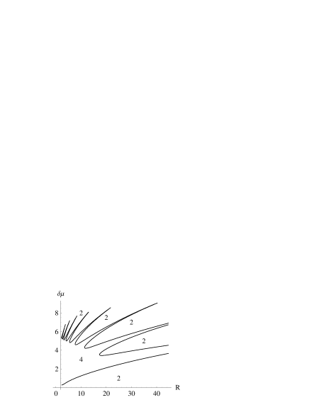
Figure 3: The phase portrait at zero temperature, $T=0$, and $m=0.01$. Number 2 denotes the chiral symmetry breaking phase with $\sigma\neq 0,\Delta=0$, and 4 denotes the mixed phase with $\sigma\neq 0$ and $\Delta\neq 0$.

The behavior of the chiral condensate $\sigma$ in the case of finite quark mass, $m\neq 0$, is shown in Fig. 4 as a function of $R$ at $\delta\mu=4.5$ (left picture) and as a function of $\delta\mu$ at $R=15$ (right picture).

$\begin{array}[]{cc}\psfig{width=227.62204pt}&\psfig{width=227.62204pt}\end{array}$

Figure 4: Condensate $\sigma$ at $\delta\mu=4.5$ (left picture) and $R=15$ (right picture), $m=0.01$

One can see oscillations of $\sigma$ on both pictures, although they are rather strong in the left picture for the dependence on $R$, while they are weakly seen in the high $\delta\mu$ tail of the curve in the right picture. One should note that the right picture resembles, except for these oscillations, the corresponding curve in [23] (Fig. 1) for the flat case.

IV.2 Finite temperature

Using formula (32) for the thermodynamic potential, we can also study the influence of finite temperature on phase transitions. The phase portrait at $T=0.1$ and zero current quark mass, $m=0$, is shown in Fig. 5 in terms of $R-\delta\mu$. It is seen from this figure that growing temperature leads to a smoothing of oscillations of the phase curve.

Figure 5: The phase portrait at $T=0.1$ and $m=0$. Number 1 denotes the symmetric phase and 3 denotes the isospin symmetry breaking phase (the phase with the pion condensate $\Delta\neq 0$).

For comparision, in Fig. 6, the phase portraits in the $T-\delta\mu$ and $R-\delta\mu$ planes (the latter now at another value of temperature $T=0.4$) are depicted. First of all, it is clear from Fig. 6 that the isospin symmetry is restored due to the vanishing of the pion condensate both at high temperature and high curvature. The similarity between these two plots leads to the conclusion that curvature and temperature effects play a similar role in the restoration of isospin symmetry.

$\begin{array}[]{cc}\psfig{width=227.62204pt}&\psfig{width=227.62204pt}\end{array}$

Figure 6: The phase portraits at $R=4$ (left picture) and at $T=0.4$ (right picture), $m=0$.

The phase portrait in Fig. 7 for $R=0$ corresponds to the case of flat Minkowski spacetime. It looks very similar to the one obtained, for instance, in [23] (see upper panel of their corresponding Fig. 12). Let us compare the phase portraits at zero (Fig. 7) and finite curvature (Fig. 6, left picture). In the first case the pion condensation appears at arbitrary small nonzero values of the isospin chemical potential, while in the second case the isospin symmetry becomes dynamically broken only at some finite value of the chemical potential $\delta\mu$. This phenomenon may be explained by the existence of a gap in the quark spectrum (23), which is proportional to the inverse radius of the Einstein universe. In this case the effect of curvature is similar to the effect of a nonzero current quark mass (for comparison see lower panel of Fig. 12 in [23] and our Fig. 6).

Figure 7: The phase portrait at $R=0$ and $m=0$.

V Conclusions

In the framework of an extended Nambu–Jona-Lasinio model, we have studied the influence of a gravitational field on pion condensation in isotopically asymmetric quark matter at finite temperature and isospin chemical potential. As a particular model of a gravitational field configuration we have taken the static Einstein universe. This particular choice enabled us to investigate phase transitions of the system with an exact consideration of the role of the gravitational field in the formation of the quark and pion condensates and thus to demonstrate its influence on the phase portraits. In particular, we have found that thermodynamic quantities such as quark and pion condensates as well as the corresponding phase boundaries (critical curves) oscillate as functions of curvature. This oscillating behavior is smoothed out with growing temperature. There exists also an interesting similarity between the behavior of phase portraits when considered as functions of curvature and as functions of finite temperature (compare Figs. 6). Moreover, we have shown that for massless quarks and for some values of $R$ the isospin symmetry becomes in curved spacetime dynamically broken only at some finite value of the chemical potential $\delta\mu$ (look at Fig. 6 (left picture) for rather small values of $T$). This is contrary to the case of flat spacetime, where the pion condensation appears at arbitrary small nonzero values of the isospin chemical potential (see Fig. 7). This effect resembles the pion condensation but at nonzero bare quark mass and may be explained by the presence of a gap in the energy spectrum of quarks in the gravitational field.

Finally, let us add some remarks on the possible role of quantum fluctuations of the collective fields and finite size effects in our approach. In fact, since the volume of the space region modelled by the closed Einstein universe adopted in this paper is limited, finite size effects could eventually change the character of phase transitions (see e.g. discussions in rubakov ; denardo ). Eventually, this might even lead to particular situations, where no phase transition can occur. However, as it is clear from physical considerations, the finite size in itself may not practically forbid the dynamical symmetry breaking, if the characteristic length of the region of space occupied by the system is much greater than the Compton wavelength of the excitation responsible for tunneling and restoration of symmetry (see, e.g., rubakov ). It should be noted that our results, obtained with the use of the mean field approximation in the framework of the NJL model are consistent with corresponding estimates of the role of quantum fluctuations (see Appendix B).

In conclusion, we emphasize that the results of this paper are evidently only of a qualitative nature. They do not allow us to find an exact value of the critical radius, and hence, further studies with more realistic models of gravitational fields should be undertaken.

Appendix A The trace of the operator $\hat{O}$ (22)

In Section III we have introduced two operators, $\hat{P}_{0}$ and $\hat{\cal H}$, acting in the Hilbert space $\mathbf{H}$ of all quadratically integrable functions $f(t,\vec{x})$ defined on the spacetime manifold of the Einstein universe.

Now suppose that there is an abstract Hilbert space $\mathbb{H}$ of vectors $|f\rangle$. Let $\hat{\vec{\mathbf{x}}}$ and $\hat{\mathbf{t}}$ be the operators of the space and time coordinates, correspondingly, defined on $\mathbb{H}$. Moreover, let $|t,\vec{x}\rangle\equiv|x\rangle$ be the complete set, or basis, of eigenvectors of $\hat{\vec{\mathbf{x}}}$ and $\hat{\mathbf{t}}$, i.e. $\hat{\vec{\mathbf{x}}}|x\rangle=\vec{x}|x\rangle$, $\hat{\mathbf{t}}|x\rangle=t|x\rangle$. The set $|x\rangle$ is usualy called the coordinate basis in $\mathbb{H}$. Obviously, the completeness and normalization conditions for the coordinate basis $|x\rangle$ are valid:

$$\int d^{4}x\sqrt{-g}|x\rangle\langle x|=\mathbf{I},$$ (33)

$$\langle x^{\prime}|x\rangle=\frac{\delta(x-x^{\prime})}{\sqrt{-g}},$$ (34)

where $\mathbf{I}$ is the unit operator in $\mathbb{H}$ and $g={\rm det}~{}g_{\mu\nu}$. Due to (33), it is possible to expand any vector $|f\rangle\in\mathbb{H}$ in terms of the basis $|x\rangle$, namely $|f\rangle=\int d^{4}x\sqrt{-g}|x\rangle\langle x|f\rangle$. The quantity $\langle x|f\rangle$ is called $x$- (or coordinate) representation for the vector $|f\rangle$. Identifying $\langle x|f\rangle$ with $f(t,\vec{x})$, we see that the Hilbert space $\mathbf{H}$ of all quadratically integrable functions is simply the coordinate representation of the above introduced abstract Hilbert space $\mathbb{H}$. Furthermore, if in the Hilbert space $\mathbb{H}$ there is an arbitrary operator $\hat{\mathbf{a}}$, then the matrix $\hat{A}$, whose matrix elements in the coordinate basis are just the quantities $\langle x^{\prime}|\hat{\mathbf{a}}|x\rangle$, is called the $x$- (or coordinate) representation of the operator $\hat{\mathbf{a}}$. Obviously, in order to define an operator $\hat{\mathbf{a}}$ in the abstract Hilbert space $\mathbb{H}$, it is sufficient to define its matrix $\hat{A}\equiv\langle x^{\prime}|\hat{\mathbf{a}}|x\rangle$, which acts in the Hilbert space $\mathbf{H}$ of all quadratically integrable functions, in the coordinate basis. It is clear that Tr$\hat{A}=$$\int d^{4}x\sqrt{-g}\langle x|\hat{\mathbf{a}}|x\rangle$.

Now, let us consider in $\mathbb{H}$ the two commuting operators $\hat{\mathbf{p}}_{0}$ and $\hat{\mathbf{h}}$ such that in the $x$-representation they look like $\hat{P}_{0}\equiv\langle x^{\prime}|\hat{\mathbf{p}}_{0}|x\rangle$ and $\hat{\cal H}\equiv\langle x^{\prime}|\hat{\mathbf{h}}|x\rangle$, correspondingly (see section III). The operators $\hat{P}_{0}$ and $\hat{\cal H}$ have a common set of eigenfunctions $\Psi_{l\alpha\eta p_{0}}(t,\vec{x})$ defined in section III, from which it follows that

$$\int d^{4}x\sqrt{-g}\Psi_{l\alpha\eta p_{0}}(t,\vec{x})\Psi^{*}_{l^{\prime}\alpha^{\prime}\eta^{\prime}p^{\prime}_{0}}(t,\vec{x})=2\pi\delta(p^{\prime}_{0}-p_{0})\delta_{ll^{\prime}}\delta_{\alpha\alpha^{\prime}}\delta_{\eta\eta^{\prime}}.$$ (35)

The eigenfunctions $\Psi_{l\alpha\eta p_{0}}(t,\vec{x})$ are the coordinates of the corresponding eigenvectors $|l\alpha\eta p_{0}\rangle\in\mathbb{H}$ of the operators $\hat{\mathbf{p}}_{0}$ and $\hat{\mathbf{h}}$ (recall, $l=0,...\infty;\alpha=1,..,d_{l}\equiv 2(l+1)(l+2);\eta=\pm 1;-\infty<p_{0}<\infty$):

$$|l\alpha\eta p_{0}\rangle=\int d^{4}x\sqrt{-g}|x\rangle\Psi_{l\alpha\eta p_{0}}(t,\vec{x})\equiv\int d^{4}x\sqrt{-g}|x\rangle\langle x|l\alpha\eta p_{0}\rangle.$$ (36)

(Clearly, $\hat{\mathbf{p}}_{0}|l\alpha\eta p_{0}\rangle=p_{0}|l\alpha\eta p_{0}\rangle$ and $\hat{\mathbf{h}}|l\alpha\eta p_{0}\rangle=\eta E_{l}|l\alpha\eta p_{0}\rangle$.) It follows from (36) that $\Psi_{l\alpha\eta p_{0}}(t,\vec{x})=\langle x|l\alpha\eta p_{0}\rangle$. Using this relation in the normalization condition (35) and then integrating there over $x$ with the help of (33), we obtain

$$\langle l^{\prime}\alpha^{\prime}\eta^{\prime}p^{\prime}_{0}|l\alpha\eta p_{0}\rangle=2\pi\delta(p^{\prime}_{0}-p_{0})\delta_{ll^{\prime}}\delta_{\alpha\alpha^{\prime}}\delta_{\eta\eta^{\prime}}$$ (37)

which is the analogue of the normalization condition (34). It is possible to show that the completness condition for the basis $|l\alpha\eta p_{0}\rangle$ follows from (37):

$$\sum_{l\alpha\eta}\int\frac{dp_{0}}{2\pi}|l\alpha\eta p_{0}\rangle\langle l\alpha\eta p_{0}|=\mathbf{I}.$$ (38)

Let us construct in $\mathbb{H}$ the following operator

$$\hat{\mathbf{o}}=\Delta^{2}-(\hat{\mathbf{p}}_{0}+\mu)^{2}+(\hat{\mathbf{h}}+\delta\mu)^{2}$$ (39)

which is diagonal in the basis (36), i.e. each vector $|l\alpha\eta p_{0}\rangle$ is its eigenvector with corresponding eigenvalue ${\cal E}_{l\alpha\eta p_{0}}$ (25). In the coordinate representation its matrix $\langle x^{\prime}|\hat{\mathbf{o}}|x\rangle$ coincides with the operator $\hat{O}$ (22). So,

$${\rm Tr}\hat{O}\equiv\int d^{4}x\sqrt{-g}\langle x|\hat{\mathbf{o}}|x\rangle=\int d^{4}x\sqrt{-g}\sum_{l\alpha\eta}\int\frac{dp_{0}}{2\pi}\sum_{l^{\prime}\alpha^{\prime}\eta^{\prime}}\int\frac{dp^{\prime}_{0}}{2\pi}\langle x|l\alpha\eta p_{0}\rangle\langle l\alpha\eta p_{0}|\hat{\mathbf{o}}|l^{\prime}\alpha^{\prime}\eta^{\prime}p^{\prime}_{0}\rangle\langle l^{\prime}\alpha^{\prime}\eta^{\prime}p^{\prime}_{0}|x\rangle,$$ (40)

where the last equality was obtained by employing the completeness relation (38). Now, by using in this formula the eigenvalue condition $\hat{\mathbf{o}}|l\alpha\eta p_{0}\rangle={\cal E}_{l\alpha\eta p_{0}}|l\alpha\eta p_{0}\rangle$, the normalization condition (37), and, finally, by performing in the obtained expression the integration and summation over primed indices, we have

$${\rm Tr}\hat{O}=\int d^{4}x\sqrt{-g}\sum_{l\alpha\eta}\int\frac{dp_{0}}{2\pi}{\cal E}_{l\alpha\eta p_{0}}\langle x|l\alpha\eta p_{0}\rangle\langle l\alpha\eta p_{0}|x\rangle=\int d^{4}x\sqrt{-g}\sum_{l\alpha\eta}\int\frac{dp_{0}}{2\pi}{\cal E}_{l\alpha\eta p_{0}}\Psi_{l\alpha\eta p_{0}}(t,\vec{x})\Psi^{*}_{l\alpha\eta p_{0}}(t,\vec{x}).$$ (41)

Since in (41) the quantities $\sqrt{-g}$ and $\Psi_{l\alpha\eta p_{0}}(t,\vec{x})\Psi^{*}_{l\alpha\eta p_{0}}(t,\vec{x})\equiv$$\psi_{l\alpha\eta}(\vec{x})\psi_{l\alpha\eta}(\vec{x})$ (the last relation is due to the notations accepted in formula (24) and below) do not depend on the time coordinate, the expression (41) is proportional to the infinite time interval ${\cal T}\equiv\int dt$. The remaining $\vec{x}$-integration in (41) gives simply unity due to the relation (24). So we have

$${\rm Tr}\hat{O}={\cal T}\sum_{l\alpha\eta}\int\frac{dp_{0}}{2\pi}{\cal E}_{l\alpha\eta p_{0}}={\cal T}\sum_{l\eta}\int\frac{dp_{0}}{2\pi}d_{l}\big{[}\Delta^{2}-(p_{0}+\mu)^{2}+(\eta E_{l}+\delta\mu)^{2}\big{]},$$ (42)

where the fact that each eigenvalue ${\cal E}_{l\alpha\eta p_{0}}$ is $d_{l}$-fold degenerated is taken into account and the notations from (23)-(25) are used. In a similar way it is possible to obtain the quantity Tr$\ln\hat{O}$:

$${\rm Tr}\ln\hat{O}={\cal T}\sum_{l\alpha\eta}\int\frac{dp_{0}}{2\pi}\ln{\cal E}_{l\alpha\eta p_{0}}={\cal T}\sum_{l\eta}\int\frac{dp_{0}}{2\pi}d_{l}\ln\big{[}\Delta^{2}-(p_{0}+\mu)^{2}+(\eta E_{l}+\delta\mu)^{2}\big{]}.$$ (43)

Appendix B The role of quantum fluctuations and finite size effects

It is well known that spontaneous symmetry breaking in low dimensional quantum field theories may become impossible due to strong quantum fluctuations of fields. The same is also true for systems that occupy a limited space volume. However, as it is clear from physical considerations, the finite size in itself may not practically forbid the spontaneous symmetry breaking, if the characteristic length of the region of space occupied by the system is much greater than the Compton wavelength of the excitation responsible for tunneling and restoration of symmetry. (Indeed, one may recall here well known physical phenomena such as the superfluidity of Helium or superconductivity of metals that are observed in samples of finite volume). This idea has been discussed for some scalar field theories in the Einstein universe for instance, in rubakov ; denardo . In this Appendix, we shall demonstrate that, under certain conditions, dynamical symmetry breaking in NJL-type models is indeed possible in the closed Einstein universe. In particular, we will show that, if the radius of the universe is large enough such that the fluctuations of quantum fields are comparatively small, the symmetry breaking obtained in the mean field approximation is not forbidden.

For illustrations, let us confine to the analogous case of the chiral condensate and consider the simplified case of the linearized Lagrangian (6) with $\mu=0,\delta\mu=0,m=0,\pi_{k}=0$,

$$\tilde{\mathcal{L}}\displaystyle=\bar{q}(i\gamma^{\nu}\nabla_{\nu}-\sigma)q-\frac{1}{4G}\sigma^{2},$$

and the corresponding partition function $Z={\rm e}^{i{\cal S}_{\rm{eff}}}$ with

$${\cal S}_{\rm{eff}}(\sigma)=-\int d^{4}x\sqrt{-g}\frac{\sigma^{2}}{4G}-i{\rm Tr}\ln(i\gamma^{\nu}\nabla_{\nu}-\sigma).$$ (44)

Now, supposing that $\sigma=\sigma_{0}+\phi$, where $\sigma_{0}$ is the vacuum expectation value of the field $\sigma$ and $\phi$ denotes its quantum fluctuation, we obtain:

$$\ln({\cal D}-\phi)\approx\ln{\cal D}-{\cal D}^{-1}\phi-\frac{1}{2}({\cal D}^{-1}\phi)({\cal D}^{-1}\phi)-\dots,$$

where ${\cal D}=i\gamma^{\nu}\nabla_{\nu}-\sigma_{0}$. Thus $Z=Z_{0}Z_{\phi}$, where $Z_{0}=\exp iS_{0}$, $S_{0}=-\int d^{4}x\sqrt{-g}V_{0}$, and

$$V_{0}=\frac{\sigma_{0}^{2}}{4G}+i\frac{1}{\int d^{4}x\sqrt{-g}}{\rm Tr}\ln{\cal D}$$ (45)

is the effective potential at $\sigma=\sigma_{0}$. The contribution of quantum fluctuations up to the $\phi^{2}$-term to the effective action $S_{\phi}$ is given by

$$Z_{\phi}\equiv\int d\phi\exp(iS_{\phi})=\int d\phi\exp\left\{-i\int d^{4}x\sqrt{-g}\frac{1}{4G}(\phi^{2}+2\sigma_{0}\phi)-{\rm Tr}({\cal D}^{-1}\phi+\frac{1}{2}({\cal D}^{-1}\phi)({\cal D}^{-1}\phi))\right\}.$$

It is evident, that in the above expansion the term linear in $\phi$ corresponds to the so-called tadpole diagram with one external $\phi$-line and the term quadratic in $\phi$ corresponds to the “polarization operator” diagram of the $\phi$ field with one fermion loop. From (45) we can write the stationarity condition and find the gap equation, $\partial V_{0}/\partial\sigma_{0}=0$,

$$\frac{\sigma_{0}}{2G}\int d^{4}x\sqrt{-g}=i{\rm Tr}{\cal D}^{-1},$$ (46)

and the linear terms in $\phi$, corresponding to the tadpole diagram, cancel out in $Z_{\phi}$. Thus, the contribution of fluctuations to the field action is given by

$$S_{\phi}=-\int d^{4}x\sqrt{-g}\frac{\phi^{2}}{4G}+{i\over 2}{\rm Tr}({\cal D}^{-1}\phi)({\cal D}^{-1}\phi).$$ (47)

Next, we shall calculate the contribution of fluctuations $\phi$ to the effective action, taking into account the quark loop in the gravitational field. (Note that this corresponds to the integral (11) and Fig.1a in [1] .) For our purpose of making estimates of the role of fluctuations, it is sufficient to limit ourselves to the consideration of fluctuations depending only on time. In this case, we can extract the necessary kinematical factor for the meson fluctuation field and then integrate over the time-component of the loop momentum in the limit of vanishing external momenta. Finally, after going to the basis for the Dirac equation in the Einstein universe (see (22)–(24)) we obtain a sum over fermion loop quantum numbers $l$ instead of an integration over momenta of free quarks made in [1] . The sum is divergent and we regularize it by the cut off $\Lambda$. In this way we obtain the effective action

$$S_{\phi}=-\int d^{4}x\sqrt{-g}\left[\frac{\phi^{2}}{4G}+\frac{3}{4\pi^{2}a^{3}}\sum_{l=0}^{\infty}e^{-\omega_{l}/\Lambda}2(l+1)(l+2)\left(-\frac{\phi^{2}}{E_{l}}+\frac{4\sigma_{0}^{2}\phi^{2}-(\partial_{t}\phi)^{2}}{4E_{l}^{3}}\right)\right],$$ (48)

where $E_{l}$ and $\omega_{l}$ are given in (23). The summation over $l$ in the first term in parenthesis in the above equation cancels out by the term $\phi^{2}/4G$, due to the stationarity condition (46)

$$1={3G\over\pi^{2}a^{3}}\sum_{l=0}^{\infty}e^{-\omega_{l}/\Lambda}2(l+1)(l+2)\frac{1}{E_{l}}.$$ (49)

After this we obtain

$$S_{\phi}=\int dt{3\over 2}\sum_{l=0}^{\infty}e^{-\omega_{l}/\Lambda}2(l+1)(l+2)\frac{1}{E_{l}^{3}}\left({1\over 4}\dot{\phi}^{2}-\sigma_{0}^{2}\phi^{2}\right),$$

or $S_{\phi}=\int dtL_{\phi}$ with the Lagrange function

$$L_{\phi}={1\over 2}\left(\dot{\phi}^{2}-4\sigma_{0}^{2}\phi^{2}\right){\cal V}{\mathcal{Z}}^{-1},$$ (50)

where ${\cal V}=\int d^{3}x\sqrt{-g}=2\pi^{2}a^{3}$ is the space volume, and the renormalization ${\mathcal{Z}}$-factor is defined as

$${\mathcal{Z}}^{-1}={3\over 4{\cal V}}\sum_{l=0}^{\infty}e^{-\omega_{l}/\Lambda}2(l+1)(l+2)\frac{1}{(\omega_{l}^{2}+\sigma_{0}^{2})^{3/2}}.$$ (51)

For comparision, let us consider the limiting case of flat space which is reached by the replacements

$$\sum_{l}\to\int dl,~{}~{}~{}(l+1)(l+2)\to\vec{p}^{2}a^{2}$$

in (51). Then the ${\mathcal{Z}}$-factor takes the form of the integral in the Euclidean spacetime

$${\mathcal{Z}}^{-1}=12\int{d^{4}p\over(2\pi)^{4}}{1\over(p_{4}^{2}+\varepsilon_{p}^{2})^{2}},$$

with $\varepsilon_{p}$ being the quark energy. This expression evidently corresponds to the similar formula for the ${\mathcal{Z}}$-factor in the flat space case considered in [1] . Next, let us perform the field renormalization $\phi={\mathcal{Z}}^{1\over 2}\phi_{r}$ in (50). Quantum fluctuations of the boson field near the ground state $\sigma_{0}$ can now be estimated, if we consider the renormalized expression (50) as the Lagrange function for a harmonic oscillator (here, we follow the idea of rubakov ) with the mass $m$ and frequency $\omega$, formally given here by the relations

$$m={\cal V},~{}~{}~{}\omega^{2}=4\sigma_{0}^{2}\equiv M^{2}.$$

Then we can estimate the quantum fluctuations as

$$\langle\phi^{2}\rangle\approx{1\over m\omega}={1\over{\cal V}2\sigma_{0}}={1\over{\cal V}M},$$

where M is the mass of the composite $\sigma$-meson. Thus, we obtain

$$\frac{\sigma^{2}_{0}}{\langle\phi^{2}\rangle}\approx a^{3}\sigma_{0}^{3}.$$ (52)

The estimate (52) gives a criterion for the role of quantum fluctuations for a system with finite volume. Clearly, quantum fluctuations can be considered negligible, if $\sigma_{0}^{2}\gg\langle\phi^{2}\rangle$. This is in agreement with the physical requirement that quantum fluctuations should be negligible if $a\sigma_{0}\gg 1$, i.e., if the radius of the universe is much greater than the Compton wavelength $\lambda=\frac{1}{M}=\frac{1}{2\sigma_{0}}$ of the $\sigma$-meson (quarks) (see also rubakov ) .

The above estimates are certainly of a qualitative nature, and hence they do not allow us to find an exact value of a critical radius such that symmetry breaking for lower values of the curvature radius of the Einstein universe is forbidden.

References

- (1) D. Ebert and M.K. Volkov, Z. Phys. C 16, 205 (1983); Yad. Fiz. 36, 1265 (1982).
- (2) D. Ebert and H. Reinhardt, Nucl. Phys. B 272, 188 (1986); D. Ebert, H. Reinhardt, and M.K. Volkov, Prog. Part. Nucl. Phys. 33, 1 (1994).
- (3) M.K. Volkov, Fiz. Elem. Chast. Atom. Yadra 17, 433 (1986); M.K. Volkov and A.E. Radzhabov, Phys. Usp. 49, 551 (2006); A.A. Andrianov, D. Espriu, and R. Tarrach, Nucl. Phys. B 533, 429 (1998); S.V. Molodtsov, A.N. Sissakian, A.S. Sorin, and G.M. Zinovjev, arXiv:hep-ph/0702178.
- (4) S.P. Klevansky, Rev. Mod. Phys. 64, 649 (1992); T. Hatsuda and T. Kunihiro, Phys. Rept. 247, 221 (1994).
- (5) D. Bailin and A. Love, Phys. Rep. 107, 325 (1984).
- (6) M. Alford, K. Rajagopal, and F. Wilczek, Phys. Lett. B 422, 247 (1998); Nucl. Phys. B 537, 443 (1999); S.V. Molodtsov and G.M. Zinovjev, Phys. Atom. Nucl. 66, 1349 (2003).
- (7) G. Nardulli, Riv. Nuovo Cim. 25N3, 1 (2002); M. Buballa, Phys. Rep. 407, 205 (2005); I.A. Shovkovy, Found. Phys. 35, 1309 (2005); T. Ohsaku, Phys. Lett. B 634, 285 (2006); M.G. Alford, A. Schmitt, K. Rajagopal, and T. Schafer, arXiv:0709.4635.
- (8) D. Blaschke, D. Ebert, K.G. Klimenko, M.K. Volkov, and V.L. Yudichev, Phys. Rev. D 70, 014006 (2004); D. Ebert, K.G. Klimenko, and V.L. Yudichev, Phys. Rev. C 72, 015201 (2005); Eur. Phys. J. C 53, 65 (2008); D. Ebert and K.G. Klimenko, Theor. Math. Phys. 150, 82 (2007).
- (9) D.T. Son and M.A. Stephanov, Phys. Atom. Nucl. 64, 834 (2001); J.B. Kogut, and D. Toublan, Phys. Rev. D 64, 034007 (2001); J.B. Kogut, and D.K. Sinclair, Phys. Rev. D 66, 014508 (2002).
- (10) M. Frank, V. Buballa, and M. Oertel, Phys. Lett. B 562, 221 (2003).
- (11) L. He, M. Jin, and P. Zhuang, Phys. Rev. D 71, 116001 (2005).
- (12) L. He, M. Jin, and P. Zhuang, Phys. Rev. D 74, 036005 (2006).
- (13) D. Ebert and K.G. Klimenko, Eur. Phys. J. C 46, 771 (2006); J. Phys. G 32, 599 (2006).
- (14) J.O. Andersen and L. Kyllingstad, arXiv:hep-ph/0701033.
- (15) A.A. Andrianov and D. Espriu, arXiv:0709.0049; M. Loewe and C. Villavicencio, Braz. J. Phys. 37, 520 (2007); J. Erdmenger, M. Kaminski, and F. Rust, arXiv:0710.0334; S. Mukherjee, M.G. Mustafa, and R. Ray, Phys. Rev. D 75, 094015 (2007); H. Abuki, M. Ciminale, R. Gatto, N.D. Ippolito, G. Nardulli, and M. Ruggieri, arXiv:0801.4254.
- (16) K.G. Klimenko, arXiv:hep-ph/9809218; D. Ebert, K.G. Klimenko, M.A. Vdovichenko, and A.S. Vshivtsev, Phys. Rev. D 61, 025005 (2000); M.A. Vdovichenko, A.S. Vshivtsev, and K.G. Klimenko, Phys. Atom. Nucl. 63, 470 (2000).
- (17) A.S. Vshivtsev, V.Ch. Zhukovsky, K.G. Klimenko, and B.V. Magnitsky, Phys. Part. Nucl. 29, 523 (1998); D. Ebert and K.G. Klimenko, Nucl. Phys. A 728, 203 (2003); T. Inagaki, D. Kimura, and T. Murata, Prog. Theor. Phys. Suppl. 153, 321 (2004); A.A. Osipov, B. Hiller, A.H. Blin, and J. da Providencia, Phys. Lett. B 650, 262 (2007); arXiv:0802.3193; T.D. Cohen, D.A. McGady, and E.S. Werbos, Phys. Rev. C 76, 055201 (2007); P. Castelo Ferreira and J. Dias de Deus, arXiv:0707.4200; E.S. Werbos, arXiv:0711.2635.
- (18) D. Ebert, K.G. Klimenko, and H. Toki, Phys. Rev. D 64, 014038 (2001); V.Ch. Zhukovsky, V.V. Khudyakov, K.G. Klimenko, and D. Ebert, Pis’ma Zh. Eksp. Teor. Fiz. 74, 595 (2001); D. Ebert et al., Phys. Rev. D 65, 054024 (2002); T. Tatsumi, E. Nakano, and K. Nawa, arXiv:hep-ph/0506002; E.J. Ferrer, V. de la Incera, and C. Manuel, Phys. Rev. Lett. 95, 152002 (2005); Nucl. Phys. B 747, 88 (2006); J.L. Noronha and I.A. Shovkovy, Phys. Rev. D 76, 105030 (2007).
- (19) D. Ebert, K.G. Klimenko, V.C. Zhukovsky, and A.M. Fedotov, Eur. Phys. J. C 49, 709 (2007); Vestn. Mosk. Univ. Fiz. Astron. 61N2, 69 (2006).
- (20) T. Inagaki, S.D. Odintsov, and T. Muta, Prog. Theor. Phys. Suppl. 127, 93 (1997) (see also further references in this review paper).
- (21) E. Elizalde, S. Leseduarte, and S.D. Odintsov, Phys. Rev. D 49, 5551 (1994); Mod. Phys. Lett. A 9, 913 (1994).
- (22) E. Elizalde, S. Leseduarte, S.D. Odintsov, and Y.I. Shilnov, Phys. Rev. D 53, 1917 (1996).
- (23) E.V. Gorbar, Phys. Rev. D 61, 024013 (1999).
- (24) T. Inagaki and K. Ishikawa, Phys. Rev. D 56, 5097 (1997).
- (25) T. Ohsaku, Phys. Lett. B 599, 102 (2004).
- (26) D. Ebert and V.Ch. Zhukovsky, Phys. Lett. B 645, 267, (2007). (The paper contains a misprint in the definition of matrices in the charge conjugation operator C, which should read like this . The results of the paper, however, were obtained with the above correct expression for this operator and do not depend on this misprint.)
- (27) T.S. Bunch and L. Parker, Phys. Rev. D 20, 2499 (1979).
- (28) L. Parker and D.J. Toms, Phys. Rev. D 29, 1584 (1984).
- (29) D.K. Kim and K.G. Klimenko, J. Phys. A 31, 5565 (1998).
- (30) A. Goyal and M. Dahiya, J. Phys. G 27, 1827 (2001).
- (31) X. Huang, X. Hao, and P. Zhuang, Astropart. Phys. 28, 472 (2007).
- (32) D. Ebert, A.V. Tyukov, and V.Ch. Zhukovsky, Phys. Rev. D 76, 064029 (2007).
- (33) J.D. Barrow, G.F.R. Ellis, R. Maartens, and C.G. Tsagas, Class. Quant. Grav. 20, L155 (2003).
- (34) J.D. Smith and D.J. Toms, Phys. Rev. D 53, 5771 (1996).
- (35) R. Camporesi, Phys. Rept. 196, 1 (1990); R. Camporesi and A. Higuchi, arXiv:gr-qc/9505009.
- (36) P. Candelas and S. Weinberg, Nucl. Phys. B 237, 397 (1984).
- (37) K.G. Klimenko, Theor. Math. Phys. 70, 87 (1987).
- (38) P. Elmfors, D. Persson, and B.S. Skagerstam, Phys. Rev. Lett. 71, 480 (1993); J.O. Andersen and T. Haugset, Phys. Rev. D 51 (1995) 3073; A.S. Vshivtsev, K.G. Klimenko, and B.V. Magnitsky, J. Exp. Theor. Phys. 80, 162 (1995); J. Exp. Theor. Phys. 82, 514 (1996).
- (39) V.Ch. Zhukovsky and J.Herrmann, Yad. Fiz. 14, 150 (1971); 14, 1014 (1971).
- (40) A.V. Veryaskin, V.G. Lapchinskii, and V.A. Rubakov, Teor. Mat. Fiz. 45, 407 (1980).
- (41) G. Denardo and E. Spalucci, Class. Quantum Grav. 6, 1915 (1989).
- (42) D. Ebert, M. Nagy, and M.K. Volkov, Yad. Fiz. 59, 149 (1996).