Geometric Polarimetry $-$ Part I: Spinors and Wave States

Abstract

A new approach to polarization algebra is introduced. It exploits the geometric properties of spinors in order to represent wave states consistently in arbitrary directions in three dimensional space. In this first expository paper of an intended series the basic derivation of the spinorial wave state is seen to be geometrically related to the electromagnetic field tensor in the spatio-temporal Fourier domain. Extracting the polarization state from the electromagnetic field requires the introduction of a new element, which enters linearly into the defining relation. We call this element the phase flag and it is this that keeps track of the polarization reference when the coordinate system is changed and provides a phase origin for both wave components. In this way we are able to identify the sphere of three dimensional unit wave vectors with the Poincaré sphere.

I Introduction

The development of applications in radar polarimetry has been vigorous over the past decade, and is anticipated to continue with ambitious new spaceborne remote sensing missions (for example TerraSAR-X [1] and TanDEM-X [2]). As technical capabilities increase, and new application areas open up, innovations in data analysis often result. Because polarization data are spatial and vectorial as well as complex, polarimetry possesses a rich mathematical background that includes not only standard electromagnetics but also linear algebra and the algebras of Hermitian forms and Lie groups [3].

Whilst the aforementioned areas are well established mathematically, the development of the formal theory of polarimetry historically has been somewhat unusual, in the sense that it has seemed to require some uncommon concepts, such as the pseudo-eigenvectors of Huynen [4], and more recently consimilarity transformations [5], [6], [7] have been invoked. There has long been a sense amongst some researchers that the theory of polarimetry requires reforming, and a number of efforts to do so have occurred over time [8], [9], [10], [11], [12], [13], [6], usually evoking controversial responses [14], [15], [16], [17]. What is quite interesting about these episodes is that expert opinion is often divided over what precisely is wrong with any new approach.

Clearly any new attempt along this road must be taken not only with care, but with a view to justifying the need for and applications of the new approach. In contrast to earlier suggested changes to the formalism which addressed quite small parts of the picture (e.g. Graves [8] and Hubbert [12]), we have taken a rather radical view. We believe that it is necessary to start ab initio $-$ essentially from the Maxwell equations. We are aware that some researchers in the discipline see no essential problem, and hence no need for a reform $-$ and they may feel quite justified in such an opinion if they continue to obtain results which work in practice. In response to this type of objection, we would counter that it is quite possible that in any given application area, a certain mathematical formulation works without any contradiction appearing. Problems can occur, however, if one tries to extend a representation to another application area where the analysis no longer work; as time goes on, it is a virtual certainty that such attempts will be made. The underlying causes of problems may be seen to lie in the very pervasiveness of polarimetry in scientific applications. The problem lies in the fact that many application areas in polarimetry either involve special cases, or avoid certain special cases $-$ for instance, the conventions used in the optical community for ellipsometry assume a fixed plane for reference, so that the transition from what radar polarimetrists would call bistatic to monostatic involve no ambiguity. In the radar community, on the contrary, a special convention is normally used such that monostatic scattering in reciprocal media involves symmetric scattering matrices. But in moving to the bistatic case, which is becoming an increasingly topical interest, there may be inequivalent mathematical representations, not all of which are equally appropriate: we address this very briefly below.

We are aware that the general polarimetric community is not primarily interested in mathematical exposition per se, and there has been some debate as to whether this is the correct forum in which to introduce our ideas. However, in our view, so much is wrong with the current state of polarimetric theory that it is necessary to explain first what is the matter with it, and preferably to provide an answer. Although this is necessarily rather theoretical, we strive to keep our development as approachable as possible. So before moving on to introduce the substance of our new approach, we offer a selection of concrete examples that demonstrate that the current conceptual framework in polarimetry is lacking, and a cause for concern for the rigor of the discipline. It should also be reasonably clear that many of the problems are linked, and must relate to something fairly fundamental. We hope that it may be seen as worthwhile to invest effort in establishing a workable theoretical basis for polarimetry.

We note, firstly, a well known identity concerning unitary matrices, namely,

$$\bar{U}^{T}=U^{-1}\quad\mbox{or}$$ (1)

$$U^{T}=\bar{U}^{-1},\quad\quad$$ (2)

where $\bar{U}$ denotes the complex conjugation of the unitary matrix $U$, and $U^{T}$ the matrix transpose. This relation in either form appears to have had, and fulfilled, its potential to cause confusion in the development and application of radar polarimetry formalism. Let us take three types of transformation law that occur in application to matrices in the literature:

$$A\;\rightarrow\;T^{-1}AT$$ (3)

$$A\;\rightarrow\;T^{T}AT$$ (4)

$$A\;\rightarrow\;\bar{T}^{-1}AT.$$ (5)

Here, we are not necessarily assuming any particular properties for transformation matrix $T$. The first of these (3) is known mathematically as a similarity, the second (4) as a congruence, and the third (5) as a consimilarity or conjugate similarity [5]. To understand why each of these might be applied in a given situation, it is helpful first to see what kind of object gets mapped to what.

In case (3), if the matrix $A$ operates on a vector $\mathbf{x}$, geometrically a point in a space, to produce another vector or point $\mathbf{x}^{\prime}$

$$\mathbf{x}^{\prime}=A\mathbf{x},$$ (6)

then the similarity transformation $T$ provides a new representation $\bar{\mathbf{x}}$ of the point $\mathbf{x}$,

$$\mathbf{x}=T\bar{\mathbf{x}}$$ (7)

such that transformed operations on transformed vectors are equivalent to operations performed on old vectors. In fact, using (6) and (7)

$$T\bar{\mathbf{x}}^{\prime}=AT\bar{\mathbf{x}}\quad\Rightarrow\quad\bar{\mathbf{x}}^{\prime}=T^{-1}AT\bar{\mathbf{x}}=\bar{A}\bar{\mathbf{x}}$$ (8)

shows that the operation $\bar{A}$ on $\bar{\mathbf{x}}$ follows the same equation of $A$ on $\mathbf{x}$ if $A$ is transformed with a similarity transformation. Moreover, the similarity applies equally correctly to a sequence of transformations $A_{1}A_{2}..$.

The geometrical interpretation of a congruence (4) is rather different. In this case the matrix $A$ describes a different type of operation altogether that maps a vector $\mathbf{x}$, geometrically a point, into an object $\mathbf{u}$ known as covector (see [19]). Geometrically covectors, according to the dimension of the space being modelled are lines in two dimensions, planes in three dimensions or hyperplanes in general $N$ dimensions, defined by $N$ points. In geometry, this operation is called correlation [19]:

$$\mathbf{u}^{\prime}=A\mathbf{x}.$$ (9)

A transformation $T$ which provides a new representation $\bar{\mathbf{x}}$ of the point $\mathbf{x}$

$$\mathbf{x}=T\bar{\mathbf{x}}$$ (10)

acts in a different way when applied to the covector $\mathbf{u}$ (see [19] for a full description):

$$\mathbf{u}=T^{-1T}\bar{\mathbf{u}}.$$ (11)

It is very clear, also from the transformation property that vectors and covectors are completely different objects, belonging to different spaces. The congruential transformation, obtained using (10) and (11)

$$T^{-1T}\bar{\mathbf{u}}^{\prime}=AT\bar{\mathbf{x}},\quad\Rightarrow\quad\bar{\mathbf{u}}^{\prime}=T^{T}AT\bar{\mathbf{x}}=\bar{A}\bar{\mathbf{x}}$$ (12)

is different from a similarity because the thing mapped and the thing mapped to are different types of objects. An important example of a correlation matrix $A$ is a quadratic form, that describes a quadratic surface, such as an ellipse in two dimensions or an ellipsoid in three. A congruence then ensures that in the transformed space, points lying on the original geometrical figure will lie on the transformed one. All this appears far abstracted from polarimetry, but will ultimately figure prominently in our development of scattering matrices, which lies out of the scope of the present paper. However, the form of (4) is instantly recognizable as that for basis transformation of a backscatter matrix (for example [9]) $-$ the only problem is to explain why theoretically such a form may be required. In the standard formalism the answer is totally obscure. Note, also, that a sequence of correlations $A_{1}A_{2}A_{3}..$ does not make mathematical sense, since the domain and range of the transformations are different types of object. The domain is constituted by proper vectors and the range by covectors.

The third example (5) which relates to consimilarity is an example of an antilinear transformation, in which vectors or points are mapped to a new space of vectors or points that involve a complex conjugation to correspond. This type of transformation is well described in the text by Horn and Johnson [5] which is regularly cited in relation to this type of transformation. It is unfortunate that, as far as we are aware, there has been no fundamental physical justification for introducing this into polarimetry. Because of (2), it is obvious that in the case of a unitary transformation, consimilarity and congruence are identical. Perhaps because of the prevalence of Hermitian forms and of unitary transformations in relation to basis change, the apparatus of quantum mechanics has had a strong influence over the mathematical development of polarimetry. But whilst mainstream quantum mechanics fundamentally involves only unitary operations on Hilbert spaces, polarimetry in the sense that it is based on classical electromagnetics, definitely does involve non-unitary processes, because scatterers and media in general can absorb. We reiterate the point that consimilarity is not a principle. Also germane to the previous point is the concept of wave-reversal. It is of course well known that, when using the same coordinate system to compare two waves that trace the same polarization ellipse, but propagate in opposite directions, the rotation of the complex vector reverses, and that in the analytic signal representation, this can be expressed by conjugation of the phasor [6]. Consequently, in the Jones vector representation [20], the vector components are conjugated for wave reversal. This is sometimes mistaken as a justification for adopting the consimilarity formalism in radar backscattering. However, it is quite clear that backscatter is not an antilinear transformation, since no time-reversal occurs. Mathematically, the operation of conjugation cannot be used selectively $-$ a point that can be missed by the unwary when analytic signal representation is used. Specifically, for the analytic representation of a harmonic plane wave, we can write

$$\overline{\mbox{e}^{j(\omega t-kz)}}=\overline{\mbox{e}^{j\omega t}}\;\overline{\mbox{e}^{-jkz}}=\mbox{e}^{j(kz-\omega t)},$$ (13)

where the overbar $\overline{\mbox{e}^{j(\omega t-kz)}}$ denotes the complex conjugate operation, $\omega$ is angular frequency and $k$ is the wavenumber. The final conjugated result has the same phase velocity as the unconjugated wave. Mathematical conjugation cannot be invoked to reverse just space or just time.

One of the most significant and useful developments in polarimetric analysis has been that of the target vector covariance theory introduced by Cloude [21], and which has been developed to a mature state [22]. Here, the starting point is a linear representation of scattering matrices $S$ using the Pauli matrix decomposition:

$$\!\!\!\!\!\!\!\!\!\!\!\!\!\!\!\!\!\!\!\!\!S=a\sigma_{0}+b\sigma_{1}+c\sigma_{2}+d\sigma_{3}=\qquad\qquad\qquad\qquad$$ (14)

$$=a\begin{pmatrix}1&\quad\!\!0\\ 0&\quad\!\!1\\ \end{pmatrix}+b\begin{pmatrix}1&\quad\!0\\ 0&-1\\ \end{pmatrix}+c\begin{pmatrix}0&\quad\!\!1\\ 1&\quad\!\!0\\ \end{pmatrix}+d\begin{pmatrix}0&-j\\ j&\quad\!0\\ \end{pmatrix},$$

where $\sigma_{l}$ are one matrix representation of the Pauli spin operators. In this, the representation of the scattering matrix is taken as a given, and the group-theoretic techniques that have arisen in this area arguably have more to do with information theoretic principles than the physics of scattering. If, however, one wishes to connect this theory to the underlying physical principles, problems can arise. It was noted in [23] that the vectorial interpretation of scattering matrices can be better related to the Poincaré sphere if the original Pauli matrix decomposition is modified. This problem can be related to the distinction between (3) and (4). Mathematically, Pauli matrices $\sigma_{l}$ are defined via multiplicative properties

$$\sigma_{l}\sigma_{m}=\delta_{lm}\sigma_{0}+j\,\varepsilon_{lmn}\sigma_{n},\quad(l,m,n=0,1,2,3)$$ (15)

where $\delta_{lm}$ is the Kronecker delta symbol and $\varepsilon_{lmn}$ is the antisymmetric Levi Civita symbol [24]. The relation (15) means that the actual realizations of the matrices are just one example of an equivalence class that transforms according to a similarity transformation. Geometrically, applying the congruential transformation (4) to the Pauli matrices makes no sense, and yet, under a basis transformation, (4) is precisely what is required. It is also a main plank of the target covariance theory that it extends to bistatic scattering by an obvious generalisation, by including the antisymmetric Pauli matrix

$$\begin{pmatrix}0&-j\\ j&\quad\!0\\ \end{pmatrix}.$$ (16)

Geometrically, however, the distinctively different Pauli matrix is $\sigma_{0}$. As [23] shows, an important simplification arises if a twisted representation is used $-$ and in fact this can be easily related to the concept of Huynen’s pseudo eigen-equation [4]. Target covariance theory ’works’ until one tries to relate it to the geometry of the Poincaré sphere. A recent example where a misunderstanding of the underlying mathematics has resulted in a very confused picture was in [25] which attempted to apply a quaternion analysis to the bistatic case, but neglected the same point. It should in fact be obvious that, within the backscatter alignment (BSA) convention, multiplication of scattering matrices makes no physical sense (for it cannot be used consistently to describe multiple scatter). Modelling scattering matrices on a division ring (the technical designation of Pauli matrices [26]) makes no sense without a fundamental modification.

To summarize the first part of our introduction, we have shown with a few examples that the mathematical and conceptual framework that pervades much of the radar polarimetry literature rests on very shaky foundations. Even if much of the analysis turns out correctly, both the physical and mathematical principles on which it rests have become obscured by a great deal of faulty reasoning over the last half century. We now commence the establishing of a new framework, which ultimately should unify the treatment of coherent and incoherent polarimetry in traditional forms and also naturally extends to the concepts of target covariance. The anticipated growth in bistatic applications suggests to us that it is timely to present such a unified theory, particularly, since it is capable of handling polarization states for waves propagating in arbitrary directions in the three dimensional space. We also hope that, once and for all, the origin of apparent idiosyncracies of polarimetric algebra will be settled.

Before going on to the main exposition, it is appropriate, given the novelty in the eyes of the polarimetric community of the formalism we employ, to say a few words concerning the scope of our objectives here and later, and the importance of what is gained. The most important single aspect of this work is emphasised by the first word in the title, which is geometric. This end is far more important than the means, which is the use of spinor algebra. If the ideas could have been presented in some other way, we would gladly have done so, however, it turns out that spinors are so perfectly adapted for representing polarimetric objects that we would otherwise have had to re-invent them. Spinors were introduced by Cartan [27] in a geometric context, and may perhaps be best summed up as doing much the same for geometry as imaginary numbers do for algebra. It may be remarked that spinors appear rather similar to Jones vectors, and the question may well arise, as to whether we are merely re-inventing them. Although these objects appear virtually identical in some contexts, there is a problem with Jones vectors in the sense that they seem to have ambiguous properties. In one sense they are extensions of Euclidean vectors, although they also may be subjected to unitary (basis) transformations. In orthogonality relations, Hermitian products are employed, whilst in antenna voltage equations a Euclidean inner product is appropriate. Mathematically, this ambiguity makes it difficult to assign any unique property, and it follows that the mathematical nature of the polarimetric model as a whole is hard to pin down rigorously. What is fundamental in this our first paper is the assignment of a coherent polarimetric state to a spinor, as a geometric entity, which turns out to be a line in projective space. Conjugate wave states are represented by conjugate spinors, and their intersections define Stokes vectors. Because spinors are truly geometric entities derived from the electromagnetic field, we are led to a quite outstanding result, that we are able to identify the Poincaré sphere with the sphere of normalised wave-vectors in the Fourier domain. Thus, no longer are polarization states (in the form of Stokes vectors) consigned to some abstract space. Rather, we can construct objects all in the same space. Given this, we can represent arbitrary geometric rotations in the same analytical framework as other polarimetric relations.

The key to achieving this will be the introduction of a hitherto ’hidden’ object, an implicit reference spinor, which we name the phase flag. This step should enable physicists to overcome their natural reticence to describe polarization vectors as spinors, which are in this algebraic form associated in field theory with ’half-spin’ particles like neutrinos. Physicists’ explanations for the $\mathrm{SU}(2)$ representation of light polarization (e.g. [28]), tend to appear half hearted and lacking conviction. In essence, when a reference spinor is taken into account, the extra half-spin required by a photon is accounted for. The amazing simplicity of this idea seems not to have surfaced in the physics literature, which probably accounts for why spinors have to date figured little in polarimetry in any formal sense. This also explains why Stokes vectors do not transform relativistically [29], even though they appear to be rather like four vectors.

Our presentation is rigorously derived from Maxwell theory for harmonic waves, and by the use of a projective formalism that extends to the spinor case [30] provides a complete and consistent geometric theory of polarization. The importance of a geometric interpretation for all the objects in polarimetry can hardly be overstated. For once one has this, algebra is only an adjunct; geometric relations remain true whatever basis transformations are applied.

This paper emerges after having worked out the implications of our ideas to a wide range of polarimetric concepts. Owing to the space required to set out the fundamentals from first principles, we limit ourselves here to the modest objective of introducing the derivation of the formalism as it applies to polarization states. We have to defer its application to scattering matrices and other entities which we hope to address in later papers. We can however assert that the geometrization of polarization leads to very simple and elegant statements about scattering matrices and their properties in a most convincing way. Ultimately, it will be seen that much of the algebra appears quite similar to that in conventional polarimetry, but the key point is that there is in the end a clarity of concept and consistency in algebraic characterization of objects that does not currently obtain.

II Spinors and geometry

The concept of polarization state has long been associated with the Poincaré sphere in a construction sometimes known as a Hopf mapping through the polarization ratio [31], that is, fundamentally, a geometric construction. The Hopf map [32] takes the points $(a,b,c,d)$ on the unit sphere in $\mathbb{R}^{4}$, labelled as $S^{3}=\{(a,b,c,d):a^{2}+b^{2}+c^{2}+d^{2}=1\}$ to points on the unit sphere in $\mathbb{R}^{3}$, labelled as $S^{2}=\{(x,y,z):x^{2}+y^{2}+z^{2}=1\}$ through the following relations:

$$x=2(ac+bd),\quad y=2(bc-ad),\quad z=a^{2}+b^{2}-c^{2}-d^{2}.$$ (17)

Introducing $\alpha=a+jb$ and $\beta=c+jd$ we have

$$a^{2}+b^{2}+c^{2}+d^{2}=1\quad\Rightarrow\quad|\alpha|^{2}+|\beta|^{2}=1.$$ (18)

We can recognize three of the Stokes parameters in $(x,y,z)$ and the components of the electric field in $(\alpha,\beta)$. Since

$$\zeta=X+jY=\frac{x-jy}{1+z}=\frac{c+jd}{a+jb}=\frac{\beta}{\alpha},$$ (19)

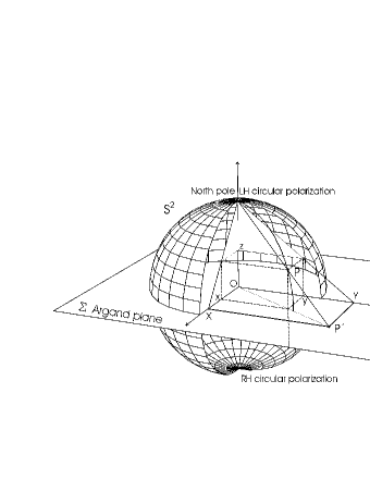
Figure 1: The stereographic projection from the Argand plane to the unit sphere in $\mathbb{R}^{3}$.

in polarimetry the Poincaré sphere is recovered through the stereographic projection, where the polarization ratio, $\zeta=\frac{\beta}{\alpha}$, is first mapped to a point on the real Argand plane and then the mapping is normally performed through the stereographic projection from the Argand plane to the unit sphere as shown in Fig. 1. The relations (20) become:

$$x=\frac{\zeta+\bar{\zeta}}{\zeta\bar{\zeta}+1},\quad y=\frac{j(\zeta-\bar{\zeta})}{\zeta\bar{\zeta}+1},\quad z=\frac{1-\zeta\bar{\zeta}}{{\zeta\bar{\zeta}+1}}.$$ (20)

and they codify the Poincaré sphere.

The aim of this paper is to perform a construction of the Poincaré sphere as a collection of complex lines and not as a Hopf map. Each coherent state of polarization will be one of the complex line generating the sphere, obtained in form of a spinor from the full electromagnetic field. Such a line can be parameterized by a complex number equivalent to the polarization ratio. The first step is now to see how a spinor can be interpreted as a generating line of a sphere, and to see the links between a sphere, a complex line and a spinor. We will attach the physical meaning to the spinor in the next sections to establish that this sphere is the Poincaré sphere.

A suitable starting point is the phase of the wave. The analytical representation of a plane wave is proportional to [34]

$$\mbox{e}^{j(\omega t-\mathbf{k}\cdot\mathbf{x})}$$ (21)

with $\omega$ the angular frenquency and $\mathbf{k}=(k_{x},k_{y},k_{z})$ the wavevector. According to relativity theory, the phase $\varphi=\omega t-\mathbf{k}\cdot\mathbf{x}$ is invariant [34]. This means that in two different reference frames (two observers in uniform relative motion) the plane wave would have different frequency $\omega$ and wavevector $\mathbf{k}$ but the phase $\varphi$ would be the same. As a consequence, the invariance of the phase corresponds to the invariance of a sort of scalar product between two vectors with four components $(\frac{\omega}{c},-k_{x},-k_{y},-k_{z})$ and $(ct,x,y,z)$:

$$\varphi=\left(\frac{\omega}{c},-k_{x},-k_{y},-k_{z}\right)\cdot(ct,x,y,z),$$ (22)

where $c$ is the speed of light in a vacuum. Because of this invariance, the frequency and the wavevector of any plane wave must form a $4-$vector. The tensor description elegantly expresses the invariance property and highlights the different behavior of the two $4-$vectors in case of change of reference frame. In fact, the $4-$vector $(ct,x,y,z)=x^{a}$ is a true vector since its dimension is a length, instead the wavevector is a $4-$gradient of a scalar invariant

$$\left(\frac{\omega}{c},-k_{x},-k_{y},-k_{z}\right)=\left(\frac{1}{c}\frac{\partial}{\partial t},\frac{\partial}{\partial x},\frac{\partial}{\partial y},\frac{\partial}{\partial z}\right)\varphi=\partial_{a}\varphi$$ (23)

which has the dimension of the inverse of a length. The $4-$vector $x^{a}$ transforms contravariantly with respect to the $4-$vector $k_{a}=(\frac{\omega}{c},-k_{x},-k_{y},-k_{z})$. The simplest demonstration of this is that if we change our unit of length from meters to centimeters, the numerical values of $x^{a}$ would scale up while those of $k_{a}$ would scale down. The tensor notation automatically takes account of this and tensors like $x^{a}$ are called contravariant while tensors like $k_{a}$ are called covariant. The tensorial notation of the product (22) would be:

$$\varphi=\sum_{a=0}^{3}k_{a}x^{a}\equiv k_{a}x^{a},$$ (24)

where we have dropped summation sign adopting the Einstein summation convention where upper indices $(x^{a})$ are paired to lower $(k_{a})$.

We shall try now to obtain representations for the complex lines generating the sphere. In order to do so, we consider now the contravariant $4-$vector $x^{a}=(\tau=ct,x,y,z)$. It is isomorphic with a Hermitian matrix which may be parameterized in the form

$$\begin{pmatrix}\tau+z&x+jy\\ x-jy&\tau-z\\ \end{pmatrix}\qquad\tau,x,y,z\in\mathbb{R}.$$ (25)

The condition that the matrix be singular may be expressed as

$$\tau^{2}-x^{2}-y^{2}-z^{2}=0.$$ (26)

In special relativity this condition is satisfied by points lying on a light-cone through the origin [35]. An alternative interpretation is for $(\tau,x,y,z)$ to be considered as homogeneous projective coordinates [19]. Let us suppose we have a point $(X,Y,Z)$ in the Euclidean space $\mathbb{R}^{3}$. To represent this same point in the projective space $\mathbb{P}^{3}$, we simply add a fourth initial coordinate: $(1,X,Y,Z)$. These coordinates are the homogenous coordinates of a point in the projective space $\mathbb{P}^{3}$. Overall scaling is unimportant, so the point $(1,X,Y,Z)$ is the same as the point $(\alpha,\alpha X,\alpha Y,\alpha Z)$. In other words,

$$(\tau,x,y,z)\equiv(\alpha\tau,\alpha x,\alpha y,\alpha z).$$ (27)

Since scaling is unimportant, if the coordinates $(\tau,x,y,z)$ are considered the homogeneous coordinates of a point in the three dimensional projective space $\mathbb{P}^{3}$, the equation (26) then defines projectively a sphere (or more generally, a quadric surface):

$$1-\left(\frac{x}{\tau}\right)^{2}-\left(\frac{y}{\tau}\right)^{2}-\left(\frac{z}{\tau}\right)^{2}=0.$$ (28)

This is reminiscent of the reduction of polarization states of arbitrary amplitude to a unit Poincaré sphere.

From one side the vanishing of the determinant of the Hermitian matrix (25) allows us to build projectively a sphere but also, since it is Hermitian, to express it [24] as the Kronecker product

$$\begin{pmatrix}\tau+z&x+jy\\ x-jy&\tau-z\\ \end{pmatrix}=$$

$$= \begin{pmatrix}\xi^{0}\\ \xi^{1}\\ \end{pmatrix}\otimes\begin{pmatrix}\bar{\xi}^{0^{\prime}}&\bar{\xi}^{1^{\prime}}\\ \end{pmatrix}=\begin{pmatrix}\xi^{0}\bar{\xi}^{0^{\prime}}&\xi^{0}\bar{\xi}^{1^{\prime}}\\ \xi^{1}\bar{\xi}^{0^{\prime}}&\xi^{1}\bar{\xi}^{1^{\prime}}\\ \end{pmatrix}\quad\xi^{0},\xi^{1}\in\mathbb{C}$$

where $\otimes$ denotes the Kronecker product, and the overbar denotes complex conjugation. The matrix on the second line in (II) built with the complex $2-$vector $(\xi^{0},\xi^{1})$ is in fact singular and Hermitian. The basic ideas here will appear familiar in polarimetric terms as relevant to the construction of the coherency matrix [36].

We can notice that the condition necessary to build a sphere projectively is the singularity of the matrix and not the Hermiticity. In fact, if we relax the Hermitian constraint we have that in general $(\tau,x,y,z)$ are not real, but they still build a singular matrix and projectively a sphere. The points $(\tau,x,y,z)$ are complex points lying on the ’real’ sphere defined as

$$\tau^{2}-x^{2}-y^{2}-z^{2}=0,\quad\tau,x,y,z\in\mathbb{C}.$$ (30)

Since the matrix is not Hermitian anymore, we have to redefine the terms of the Kronecker product (II)

$$\begin{pmatrix}\tau+z&x+jy\\ x-jy&\tau-z\\ \end{pmatrix}=$$

$$= \begin{pmatrix}\xi^{0}\\ \xi^{1}\\ \end{pmatrix}\otimes\begin{pmatrix}\bar{\eta}^{0^{\prime}}&\bar{\eta}^{1^{\prime}}\\ \end{pmatrix}=\begin{pmatrix}\xi^{0}\bar{\eta}^{0^{\prime}}&\xi^{0}\bar{\eta}^{1^{\prime}}\\ \xi^{1}\bar{\eta}^{0^{\prime}}&\xi^{1}\bar{\eta}^{1^{\prime}}\\ \end{pmatrix}\quad\!\!\tau,x,y,z\in\mathbb{C}.$$

For general complex pairs $(\xi^{0},\xi^{1})$, $(\eta^{0},\eta^{1})$, the matrix is still singular but not Hermitian. Now if $(\eta^{0},\eta^{1})$ be fixed, it can be seen that points

$$(\tau,x,y,z)$$ (32)

form a linear one dimensional, complex projective subspace, $(\xi^{0},\xi^{1})$ being variable. We want to show now that this one dimensional projective space is a complex line generating the sphere. This is the main result of this section. We will use this conclusion to define the polarization state and the Poincaré sphere in the next sections. It should be clear that the same argument may be applied keeping $(\xi^{0},\xi^{1})$ constant and varying $(\eta^{0},\eta^{1})$. In this way, a second line is generated. Every single independent $(\xi^{0},\xi^{1})$ $(\eta^{0},\eta^{1})$ pair results in a unique point of the sphere.

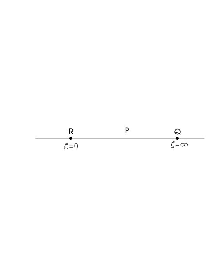
Figure 2: A ”real” visualization of the complex line. $P=R+\zeta Q$ is any point on the line. For $\xi^{1}=0$ $(\zeta=0)$, the point $P$ coincides with $R$, and for $\xi^{0}=0$ $(\zeta=\infty)$ $P\equiv Q$.

The singularity of the matrix (II) implies the existence of a sphere in the projective space $\mathbb{P}^{3}$. We want now to see what is projectively the complex $2-$vector $(\xi^{0},\xi^{1})$. As usual, we consider $(\xi^{0},\xi^{1})$ as homogeneous coordinate, which means that $(1,\zeta=\frac{\xi^{1}}{\xi^{0}})$ or any non-zero multiples of it, represents projectively the same vector. So we associate the vectors $(\xi^{0},\xi^{1})$ ($\xi^{0}\neq 0$) with all the complex numbers together with the infinity $(0,1)$ and we obtain a space which is usually labelled as $\mathbb{C}\mathbb{P}^{1}$ [19]. Regarding the dimension of this space, this depends on the point of view. From the perspective of the real numbers already $\mathbb{C}$ is a two-dimensional object often called the Argand plane. As we have already noticed in polarimetry theory this is the traditional way to arrive at the Poincaré sphere, where $\zeta$ might be interpreted as a polarization ratio. However, there is the other perspective, the complex perspective, from which $\mathbb{C}$ is just a one dimensional space. It contains just one complex parameter. In the same way as $\mathbb{R}$ is the real numbers line, one would consider $\mathbb{C}$ as the complex numbers line and so $\mathbb{C}\mathbb{P}^{1}$ is called the complex projective line. The elements of $\mathbb{C}\mathbb{P}^{1}$ are the complex $2-$vectors $(\xi^{0},\xi^{1})$, known as spinors and represented by a complex line. The point $P$ on the line is represented by the projective parameter $\zeta=\frac{\xi^{1}}{\xi^{0}}$ once two reference points $R$ and $Q$ have been chosen (see Fig. 2):

$$P=\xi^{0}R+\xi^{1}Q,\quad\Rightarrow\quad P=R+\zeta Q.$$ (33)

At this point we have a complex projective line and a projective sphere linked by the relation (II). We want now to discover the geometric significance of this link: it illustrates an example in the theory of projective geometry that through any point on a quadric surface there pass two lines, each of which lies entirely within the surface [37]. To those unfamiliar with complex geometry it may appear surprising that a sphere contains straight lines: this is a fact that escapes us because on a sphere or any quadric with positive curvature only one point on each such line is real; all other points are complex. A simple way to ”see” how a complex line can belong to the sphere is to consider planes intersecting the sphere. We consider for simplicity a sequence of planes parallel to the $xy-$plane, cutting the $z-$axis at $z_{c}$. The equation in the plane of intersection

$$x^{2}+y^{2}=1-z_{c}^{2}$$ (34)

is the equation of a circle which degenerates in a point of tangency ($z_{c}=\pm 1$). In this case, the point of tangency is not the whole solution. In fact, we have also two intersecting complex lines with gradient $\pm j$

$$x^{2}+y^{2}=0\quad\Rightarrow\quad x=\pm jy$$ (35)

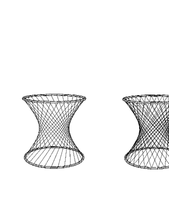
Figure 3: A quadric surface in the form of a hyperboloid. On the left we can see the hyperboloid generated by one line rotating around one axis. In the picture on the right we show the two family of generators.

having one real point $(1,0,0,1)$ at their intersection. What is surprising is that the two lines lie completely on the sphere surface. In fact, each point on these lines has coordinate $(1,\pm jy,y,1)$ which belongs to the sphere. This is a simple example to illustrate that a sphere contains complex points (30) and in particular lines built up with complex points! Now, the next step is to see how such lines can generate the sphere surface. Since it is difficult to imagine this we can consider instead a quadric surface with negative curvature. For such quadric surfaces, the generating lines can be wholly real, a fact that is exploited architecturally, e.g. in the design of cooling towers as cylindrical hyperboloids [38]. In Fig. 3 we show how a line can generate an hyperboloid. We can easily see that i) any point of the generating line is a point of the surface, ii) there are two families of generators, and through each point of the surface there pass two generators, one of each family, iii) generators of the same family do not intersect, iv) each line of one family intersects with every other line of the other family.

The point of the preceding discursive outline is to emphasize the central principle of geometric polarimetry, which is to identify the complex $2-$vectors such as

$$\xi^{A}=(\xi^{0},\xi^{1})$$ (36)

with one of the two sets of complex lines generating the sphere. The complex $2-$vector $\xi^{A}$ is known as a spinor [39], [27], [40]. We should stress at this stage that the sphere in question is to be thought of as the sphere of real unit vectors in three-dimensional space. The concept of Poincaré sphere will be derived later.

In order to establish the notation that we will use in the sequel of the paper, since the singular matrix (II) is the outer product of two spinors $\xi^{A}$ and the conjugate of $\eta^{B}$, we can label it as follows:

$$\xi^{A}\bar{\eta}^{B^{\prime}}=X^{AB^{\prime}}\equiv\begin{pmatrix}X^{00^{\prime}}&X^{01^{\prime}}\\ X^{10^{\prime}}&X^{11^{\prime}}\\ \end{pmatrix}=\begin{pmatrix}\tau+z&x+jy\\ x-jy&\tau-z\\ \end{pmatrix}.$$ (37)

We can notice that $X^{AB^{\prime}}$ is considered as a spinor with two indices; generally spinors can, like tensors have any number of indices.

We have started from the phase of a plane wave built up with two $4-$vectors, $x^{a}$ and $k_{a}$. But so far we have considered only the contravariant coordinate $4-$vector $x^{a}$ in the physical space. Now since $k_{a}$ is also a $4-$vector we can think to make the same considerations we have done for $x^{a}$. However, there is a difference. The $4-$vector $k_{a}$ is covariant. Contravariant and covariant $4-$vectors are called duals of each other. We want to explore the meaning of duality in the projective context. First, we consider the equation of a plane in the three dimensional Euclidean space:

$$f(x,y,z)=ux+vy+wz+q=0.$$ (38)

The normal vector to the plane is given by

$$\mathbf{N}=\mathbf{\nabla}f=(u,v,w).$$ (39)

The plane may be characterized via its normal vector from the origin, so a set of three coordinates $(u,v,w)$ can refer to a plane rather than a point, giving rise to a ’dual’ interpretation. If we consider the projective space, we add a fourth initial coordinate and we have that the condition:

$$\begin{pmatrix}\sigma\\ u\\ v\\ w\\ \end{pmatrix}^{T}\cdot\begin{pmatrix}\tau\\ x\\ y\\ z\\ \end{pmatrix}=\sigma\tau+ux+vy+wz=0$$ (40)

may be seen as the condition for a plane $(\sigma,u,v,w)$ to pass through the point $(\tau,x,y,z)$. Comparing (40) with (38) we have that $q=\sigma\tau$. Since the set of homogeneous coordinates $(\sigma,u,v,w)$ are defined as a gradient (39) we associate it with a covariant $4-$vector $q_{a}$ and we associate the set of coordinate $(\tau,x,y,z)$ interpreted as a point with a contravariant $4-$vector $x^{a}$. The linear equation of a plane (40) can be written as $q_{a}x^{a}=0$, with $q_{a}=(\sigma,u,v,w)$. Hence the components of any covariant vector $q_{a}$ are to be regarded as the coordinate of a plane.

Reconsidering the phase of the wave (23), the zero phase

$$k_{a}x^{a}=0\quad\Rightarrow\quad\begin{pmatrix}\frac{\omega}{c}\\ -k_{x}\\ -k_{y}\\ -k_{z}\\ \end{pmatrix}^{T}\cdot\begin{pmatrix}\tau\\ x\\ y\\ z\\ \end{pmatrix}=0$$ (41)

in the projective representation states that the plane $k_{a}$ passes through the point $x^{a}$ which belong to the sphere $1-\left(\frac{x}{\tau}\right)^{2}-\left(\frac{y}{\tau}\right)^{2}-\left(\frac{z}{\tau}\right)^{2}=0$.

At this point, we can make the same consideration we have done for $x^{a}$ keeping in mind that $k_{a}\equiv(\frac{\omega}{c},-k_{x},-k_{y},-k_{z})$ is a plane.

The singularity of the Hermitian matrix

$$K_{AB^{\prime}}\equiv\begin{pmatrix}K_{00^{\prime}}&K_{01^{\prime}}\\ K_{10^{\prime}}&K_{11^{\prime}}\\ \end{pmatrix}\equiv\begin{pmatrix}\;\;\;k_{0}-k_{z}&-k_{x}+jk_{y}\\ -k_{x}-jk_{y}&\;\;\;k_{0}+k_{z}\\ \end{pmatrix}.$$ (42)

defines projectively a sphere

$$1-\left(\frac{k_{x}}{k_{0}}\right)^{2}-\left(\frac{k_{y}}{k_{0}}\right)^{2}-\left(\frac{k_{z}}{k_{0}}\right)^{2}=0$$ (43)

with $k_{0}=\frac{\omega}{c}$. The sphere this time is an envelope of tangent planes $k_{a}$. The singularity of the matrix (42) can be expressed as:

$$k_{a}\Omega^{ab}k_{b}=0\;\mapsto\;\begin{pmatrix}\,k_{0}\\ \,k_{1}\\ \,k_{2}\\ \,k_{3}\\ \end{pmatrix}^{T}\begin{pmatrix}1&\quad\!0&\quad\!0&\quad\!0\\ 0&-1&\quad\!0&\quad\!0\\ 0&\quad\!0&-1&\quad\!0\\ 0&\quad\!0&\quad\!0&-1\\ \end{pmatrix}\begin{pmatrix}\,k_{0}\\ \,k_{1}\\ \,k_{2}\\ \,k_{3}\\ \end{pmatrix}=0$$ (44)

where $k_{1}=-k_{x}$, $k_{2}=-k_{y}$, $k_{3}=-k_{z}$, so that from here on numerical as well as symbolic index positions are to be explicitly interpreted as contravariant $x^{a}$ or covariant $k_{a}$ according to the position. We shall refer to $\Omega^{ab}$ as the wave sphere, since (44) expresses the Fourier transform of the wave equation in free space. Now we can also give a projective meaning to $k^{a}=\Omega^{ab}k_{b}=(k_{0},k^{1}=k_{x},k^{2}=k_{y},k^{3}=k_{z})$ as the point of tangency of the plane $k_{b}$ on the sphere $\Omega^{ab}$. In the Fourier domain, the interpretation of the $4-$vectors $k_{a}$ as homogeneous coordinates in three-dimensional projective space implies normalization of the frequency

$$k_{a}\;\rightarrow\;\left(1,\frac{k_{1}}{k_{0}},\frac{k_{2}}{k_{0}},\frac{k_{3}}{k_{0}}\right).$$ (45)

As we consider harmonic waves individually, and in many applications a quasi monochromatic assumption is justified this creates few problems. In return, the interpretation of the linear algebra as three-, rather then four-dimensional is beneficial from the point of view of visualization.

As for $X^{AB^{\prime}}$ in (37), the singularity of the matrix (42), allow us to express it as the Kronecker product

$$K_{AB^{\prime}}=\begin{pmatrix}\>K_{00^{\prime}}&K_{01^{\prime}}\\ \>K_{10^{\prime}}&K_{11^{\prime}}\\ \end{pmatrix}=\begin{pmatrix}\kappa_{0}\\ \kappa_{1}\\ \end{pmatrix}\otimes\begin{pmatrix}\bar{\lambda}_{0^{\prime}}&\bar{\lambda}_{1^{\prime}}\\ \end{pmatrix}$$ (46)

this time with the covariant spinors

$$\kappa_{A}=(\kappa_{0},\kappa_{1})\quad\mbox{and}\quad\lambda_{A}=(\lambda_{0},\lambda_{1}).$$ (47)

Like the contravariant spinor (36) they also represent complex lines on the sphere. The concept of duality is still valid for spinors, namely covariant and contravariant spinors are still duals of each other. However, in the three dimensional projective space $\mathbb{P}^{3}$, the dual of a line is a line or lines are self-dual. In fact, a line can be built linking two points but also it is the intersection of two planes, duals of points. Given two points $p^{a}=(p^{0},p^{1},p^{2},p^{3})$ and $q^{a}=(q^{0},q^{1},q^{2},q^{3})$ in homogeneous coordinates, the projective description of the line passing through the two points are given by the numbers:

$$p^{i}q^{j}-p^{j}q^{i}$$ (48)

which build the tensor

$$l^{ab}=p^{a}q^{b}-q^{a}p^{b}.$$ (49)

Since $l^{\,ab}=-\,l^{\,ba}$ the tensor is clearly skew-symmetric:

$$l^{\,ab}=\begin{pmatrix}0&-l^{\,10}&-l^{\,20}&-l^{\,30}\\ l^{\,10}&0&l^{\,12}&-l^{\,31}\\ l^{\,20}&-l^{\,12}&0&l^{\,23}\\ l^{\,30}&l^{\,31}&-l^{\,23}&0\\ \end{pmatrix}$$ (50)

and therefore the distinct elements are reduced to six

$$\{l^{\,10},l^{\,20},l^{\,30},l^{\,23},l^{\,31},l^{\,12}\}.$$ (51)

However, they are not independent since they always satisfy

$$l^{\,10}l^{\,23}+l^{\,20}l^{\,31}+l^{\,30}l^{\,12}=0$$ (52)

which is the determinant of a $4\times 4$ matrix $(p^{a},q^{a},p^{a},q^{a})$ that is identically zero. The coordinates (51) connected by the relation (52) are called Pluecker (or Grassmann) coordinates of a line. Again overall scaling is unimportant, namely the set

$$\{\alpha\,l^{\,10},\alpha\,l^{\,20},\alpha\,l^{\,30},\alpha\,l^{\,23},\alpha\,l^{\,31},\alpha\,l^{\,12}\}$$ (53)

represents the same line as (51) does. If the first coordinate of the points is not zero, it is easy to show that the coordinates have a nice Euclidean interpretation, namely

$$\begin{array}[]{l}(l^{\,10},l^{\,20},l^{\,30})=\mathbf{p}-\mathbf{q}\\ (l^{\,23},l^{\,31},l^{\,12})=\mathbf{p}\times\mathbf{q}\\ \end{array}$$ (54)

with $\mathbf{p}=(\frac{p^{1}}{p^{0}},\frac{p^{2}}{p^{0}},\frac{p^{3}}{p^{0}})$, $\mathbf{q}=(\frac{q^{1}}{q^{0}},\frac{q^{2}}{q^{0}},\frac{q^{3}}{q^{0}})$ and where $\times$ denotes the cross product. The first set of coordinates describes the direction of the line from $\mathbf{q}$ to $\mathbf{p}$ and the second describes the plane containing the line and the origin. The condition (52) is equivalent to the identically null product

$$(\mathbf{p}-\mathbf{q})\cdot(\mathbf{p}\times\mathbf{q})$$ (55)

where $\cdot$ denotes the scalar product.

Alternatively, we consider the planes $p_{a}=\Omega_{ab}p^{b}$ and $q_{a}=\Omega_{ab}q^{b}$. We define the skew-symmetric tensor $l_{ab}$

$$l_{ab}=p_{a}q_{b}-q_{a}p_{b}$$ (56)

whose components are related to the components of $l^{\,ab}$ in (49)

$$l_{ab}=\Omega_{ac}\Omega_{bd}l^{\,cd}=\begin{pmatrix}0&l^{\,10}&l^{\,20}&l^{\,30}\\ -l^{\,10}&0&l^{\,12}&-l^{\,31}\\ -l^{\,20}&-l^{\,12}&0&l^{\,23}\\ -l^{\,30}&l^{\,31}&-l^{\,23}&0\\ \end{pmatrix}$$ (57)

which is the dual of the tensor ${}^{*}r_{ab}$ representing the line intersection of the planes $p_{a}$ and $q_{a}$:

$$^{*}r_{ab}=l_{ab}.$$ (58)

The dual of a tensor is defined through the full antisymmetric Levi Civita symbol $\varepsilon^{abcd}$ and it is related to the tensor $r^{\,ab}$ :

$$r^{\,ab}=-\frac{1}{2}\,\varepsilon^{abcd}\,{}^{*}r_{cd}$$ (59)

which components can be written in function of the components of $l^{ab}$:

$$r^{\,ab}=\begin{pmatrix}0&-l^{\,23}&-l^{\,31}&-l^{\,12}\\ l^{\,23}&0&-l^{\,30}&l^{\,20}\\ l^{\,31}&l^{\,30}&0&-l^{\,10}\\ l^{\,12}&-l^{\,20}&l^{\,10}&0\\ \end{pmatrix}.$$ (60)

The Pluecker coordinates of the line intersection of $p_{a}$ and $q_{a}$ will be the set:

$$\{l_{23},l_{31},l_{12},-l_{10},-l_{20},-l_{30}\}.$$ (61)

Again considering the Euclidean interpretation as in (62), the vector $\mathbf{p}$ and $\mathbf{q}$ now represents the normal to the planes. For this reason

$$\begin{array}[]{l}(l^{\,23},l^{\,31},l^{\,12})=\mathbf{p}\times\mathbf{q}\\ (-l^{\,10},-l^{\,20},-l^{\,30})=\mathbf{q}-\mathbf{p}\\ \end{array}$$ (62)

this time the first set of coordinates namely the direction of the line is described by $\mathbf{p}\times\mathbf{q}$ and the second set namely the plane containing the line and the origin is described by $\mathbf{q}-\mathbf{p}$. We emphasize that this is only an Euclidean interpretation that can help us to visualize things but the Pluecker coordinates are coordinates in the projective space and not in the Euclidean space.

III The algebra of spinors

In the previous section we introduced contravariant and covariant spinors by interpreting them as representations of the complex lines generating the sphere. In this section we will discuss the algebra of spinors especially the relation between covariant and contravariant spinors and the conjugate spinors.

Spinors were first introduced by Cartan [27] in 1913 and later they were adopted in quantum mechanics to study the properties of the intrinsic angular momentum of the electron and other fermions. Today spinors are used in a wide range of branches of physics and mathematics.

This paper follows the notations and the conventions of the book by Penrose and Rindler [33] which provides a very clear idea of what spinor representation signifies.

The spinor $\xi^{A}$ has four basic forms each of which follows a separate and distinguished transformation law. This is the strength of the spinor notation, especially for polarimetry: the labelling of a spinor of one of the four type immediately dictates its transformation properties.

Many of the equations of polarimetry involve nothing more complicated than $2\times 2$ complex matrices. By understanding the significance of spinor index types, it becomes clear that these are potentially $4\times 4$ different characters of $2\times 2$ complex matrices; little wonder therefore that confusion may arise over the correct transformation laws!

We start now to describe the four forms of a spinor and their transformation law, and later after the derivation of the polarization state from the electromagnetic field tensor we will show why and how the distinction of the same object in four forms is fundamental in polarimetry. The four spinor types can be categorized as:

• the contravariant spinor $\xi^{A}$,

• the covariant spinor $\xi_{A}$,

• the conjugate contravariant spinor $\bar{\xi}^{A^{\prime}}$,

• the conjugate covariant spinor $\bar{\xi}_{A^{\prime}}$.

All these different types have definite and different physical or geometric significance, and must not be confused with one another.

In the next two sections we describe how to raise and lower indexes and the conjugation of a spinor. The significance of raising and lowering is to make a relation between one type and another. This can be seen as a mapping between objects that are dual to one another through some fixed geometric property.

III-A Index raising and lowering

In this section we introduce the metric spinor $\epsilon_{AB}=\epsilon^{AB}$ which tells us how to compute distances in spinor space. We will see that it is the object responsible for lowering and raising the indexes and which can test the independence of two given spinors.

We have seen in the previous section that projectively the following components of a spinor are equivalent:

$$\begin{pmatrix}\xi^{0}\\ \xi^{1}\\ \end{pmatrix}\equiv\begin{pmatrix}1\\ \frac{\xi^{1}}{\xi^{0}}\\ \end{pmatrix}=\begin{pmatrix}1\\ \zeta\\ \end{pmatrix}.$$ (63)

The spinor components $(\xi^{0},\xi^{1})$ may be interpreted as the homogeneous coordinate of a point $P$ on a complex line (see Fig. 2). Then the complex number $\zeta$ is the inhomogeneous coordinate of the point on the complex line known as the affine coordinate of a point. Following this terminology we can see that the difference between complex numbers $\xi$, $\eta$, namely the affine distance between the two points $P-P^{\prime}$ may be expressed in terms of their homogeneous coordinates as

$$\xi-\eta=\left[\begin{pmatrix}\quad\!0&1\\ -1&0\\ \end{pmatrix}\begin{pmatrix}1\\ \xi\\ \end{pmatrix}\right]^{T}\begin{pmatrix}1\\ \eta\\ \end{pmatrix}.$$ (64)

Now reinterpreting the same relation using the homogeneous coordinates we can recover the invariant skew-symmetric spinor $\epsilon_{AB}$ called metric spinor:

$$\left[\begin{pmatrix}\quad\!0&1\\ -1&0\\ \end{pmatrix}\begin{pmatrix}\eta^{0}\\ \eta^{1}\\ \end{pmatrix}\right]^{T}\begin{pmatrix}\xi^{0}\\ \xi^{1}\\ \end{pmatrix}\equiv\epsilon_{AB}\xi^{A}\eta^{B},$$ (65)

where we adopt as usual the Einstein summation convention. The metric spinor has components

$$\epsilon_{AB}\quad\rightarrow\quad\epsilon_{12}=-\epsilon_{21}=1,\quad\epsilon_{11}=\epsilon_{22}=0$$ (66)

namely it is a completely antisymmetric spinor ($\epsilon_{AB}=-\epsilon_{BA}$).

Since the distance is always related to some kind of product, we can symbolically introduce the inner product

$$\epsilon_{AB}\xi^{A}\eta^{B}=\xi_{B}\eta^{B},$$ (67)

where the covariant spinor $\xi_{B}$

$$\xi_{B}=\epsilon_{AB}\xi^{A},\quad\begin{pmatrix}\xi_{0}\\ \xi_{1}\\ \end{pmatrix}=\begin{pmatrix}-\xi^{1}\\ \quad\!\xi^{0}\\ \end{pmatrix}$$ (68)

is obtained from the contravariant one with the lowering operator $\epsilon_{AB}$. Here, as usual, we use the Einstein summation convention.

Likewise, $\epsilon^{AB}$ which has numerically the same element values as $\epsilon_{AB}$ is a raising operator, performing the inverse mapping from covariant space to contravariant:

$$\xi^{A}=\epsilon^{AB}\xi_{B}.$$ (69)

We note that

$$\epsilon_{AB}\,\epsilon^{CB}=\epsilon_{A}^{\;\;C}$$ (70)

is the Kronecker delta symbol $\delta_{A}^{\;\;C}$ in spinor space.

It may also be recognized that the product (67) vanishes if the ratios of the spinor coordinates of $\xi=\frac{\xi_{1}}{\xi_{0}}$ and $\eta=\frac{\eta_{1}}{\eta_{0}}$ are equal, namely

$$\xi_{B}\eta^{B}=0\quad\Leftrightarrow\quad\xi^{B}\propto\eta^{B}.$$ (71)

Geometrically, if the two points on the line coincide, the distance vanishes. So, we have arrived at a symbolic mechanism for testing the linear independence of two spinors:

$$\xi_{A}\eta^{A}\neq 0.$$ (72)

We want finally to show how spinors transform for linear transformations. Since linear transformations map contravariant spinors to contravariant, we can express the transformation law for a spinor as

$$\xi^{A}\quad\rightarrow\quad\tilde{\xi}^{A}=L^{A}_{\;\;B}\xi^{B}.$$ (73)

with $L^{A}_{\;\;B}$ the spinor describing the linear transformation. Using their matrix representation we can write:

$$\begin{pmatrix}\xi^{0}\\ \xi^{1}\\ \end{pmatrix}\quad\rightarrow\quad\begin{pmatrix}\tilde{\xi}^{0}\\ \tilde{\xi}^{1}\\ \end{pmatrix}=\begin{pmatrix}L^{0}_{\;\;0}&L^{0}_{\;\;1}\\ L^{1}_{\;\;0}&L^{1}_{\;\;1}\\ \end{pmatrix}\begin{pmatrix}\xi^{0}\\ \xi^{1}\\ \end{pmatrix},$$ (74)

where $L^{A}_{\;\;B}$ is represented by a $2\times 2$ matrix.

III-B Conjugate spaces

In the last section we have introduced two types of spinors, the contravariant and the covariant and their transformation law. The other two kinds of spinors are the ’primed’ ones belonging to the conjugate space. Thus,

$$\overline{\eta^{A}}=\bar{\eta}^{A^{\prime}}\equiv\begin{pmatrix}\bar{\eta}^{0^{\prime}}\\ \bar{\eta}^{1^{\prime}}\\ \end{pmatrix}$$ (75)

in which the numerical values of the components are conjugated, and the abstract index becomes primed. The conjugate spinor $\bar{\eta}^{A^{\prime}}$ will transforms according to the conjugate law

$$\bar{\tilde{\eta}}^{A^{\prime}}=\bar{L}^{A^{\prime}}_{\;\;B^{\prime}}\bar{\eta}^{B^{\prime}}$$ (76)

where $\bar{L}^{A^{\prime}}_{\;\;B^{\prime}}$ is the conjugate transformation. The operation of priming applies equally to covariant spinors, so we have obtained the four categories of spinors: $\eta^{A}$, $\eta_{A}$, $\bar{\eta}^{A^{\prime}}$, $\bar{\eta}_{A^{\prime}}$.

Using the explicit transformation laws for the four types of spinors we can infer the transformation law for spinors with more indices and see why attaching the prime in the index is necessary.

In section II we have considered matrices expressible as a Kronecker product of two spinors (37)

$$\xi^{A}\bar{\eta}^{B^{\prime}}=X^{AB^{\prime}}.$$ (77)

Now using the transformation law (73) and (76) for $\xi^{A}$ and for $\bar{\eta}^{B^{\prime}}$ we can show that $X^{AB^{\prime}}$ transforms not simply as a matrix but

$$X^{AB^{\prime}}\quad\rightarrow\quad\tilde{X}^{AB^{\prime}} = \tilde{\xi}^{A}\bar{\tilde{\eta}}^{B^{\prime}}=L^{A}_{\;\;C}\,\xi^{C}\bar{\eta}^{D^{\prime}}\bar{L}^{B^{\prime}}_{\;\;D^{\prime}}=$$ (78)

$$= L^{A}_{\;\;C}\,X^{CD^{\prime}}\,\bar{L}^{B^{\prime}}_{\;\;D^{\prime}}.$$

Expressing the relation below with the matrix representation we can rewrite it as:

$$X\quad\rightarrow\quad\tilde{X}=LX\bar{L}^{T},$$ (79)

where $X$ is the matrix representing $X^{AB^{\prime}}$ and $\bar{L}^{T}$ is the conjugate transpose of the matrix representing $L^{A}_{\;\;B}$.

We can easily see that the prime attached to the index is very essential in order to keep trace of the fact that they transform with the conjugate transformation. Clearly, since conjugation is an involutory operation, it means that a double primed label reverts to the unprimed.

Through an example we can see that if $L$ is a rotation in space, $X^{AB^{\prime}}$ (and consequently the $4-$vector) rotates by double the angle of rotation of a spinor. Since the group of unitary transformation $\mathrm{SU}(2)$ is the universal covering group of the orthogonal rotation group $\mathrm{SO}(3)$, this means that there is a correspondence between elements of $\mathrm{SU}(2)$ and of $\mathrm{SO}(3)$. The unitary transformation can be expressed with the Cayley-Klein parameters in terms of the Euler angles $\psi$, $\theta$ and $\varphi$ for the rotation considered [41]:

$$U^{A}_{\;\;B}\equiv\begin{pmatrix}\cos\frac{\theta}{2}\,\mbox{e}^{j\frac{\psi+\varphi}{2}}&j\sin\frac{\theta}{2}\,\mbox{e}^{j\frac{\psi-\varphi}{2}}\\ j\sin\frac{\theta}{2}\,\mbox{e}^{-j\frac{\psi-\varphi}{2}}&\cos\frac{\theta}{2}\,\mbox{e}^{-j\frac{\psi+\varphi}{2}}\\ \end{pmatrix}.$$ (80)

The example is a rotation in space around the $z$ direction by angle $\alpha$. The unitary spinor is in this case

$$U^{A}_{\;\;B}\equiv\begin{pmatrix}\mbox{e}^{-j\frac{\alpha}{2}}&0\\ 0&\mbox{e}^{j\frac{\alpha}{2}}\\ \end{pmatrix}.$$ (81)

According to (73), the new spinor $\tilde{\xi}^{A}$ after the rotation will be:

$$\tilde{\xi}^{A}=U^{A}_{\;\;B}\,\xi^{B}=\begin{pmatrix}\mbox{e}^{-j\frac{\alpha}{2}}\,\xi^{0}\\ \mbox{e}^{j\frac{\alpha}{2}}\,\xi^{1}\\ \end{pmatrix}.$$ (82)

For $\alpha=2\pi$ this rotation brings back to the original value $X^{AB^{\prime}}$ (according to (78)) but reverses the sign of the spinor $\xi^{A}$.

A MATHEMATICA package [42] has been developed in order to perform symbolic calculation with spinors and tensors for radar polarimetry using the Penrose-Rindler notation [33].

In our view, the correct attribution of covariant, contravariant, and primed or unprimed is crucial to a proper understanding of polarimetric transformation properties. A particular source of confusion in polarimetry arises from a restricted symmetry, in that for any spinor $\xi^{A}$, $\bar{\xi}_{A^{\prime}}$ has numerically the same components up to a phase factor as the ’orthogonal’ spinor. In fact, two independent spinors satisfy (72). In particular, if

$$\xi_{A}\eta^{A}=1,$$ (83)

the pair $\{\xi^{A},\eta^{A}\}$ forms a spin frame which allows any spinors to be represented in components. The spinor $\eta^{A}$ then will have components

$$\eta^{A}=\begin{pmatrix}-\bar{\xi}^{1^{\prime}}\\ \quad\!\bar{\xi}^{0^{\prime}}\\ \end{pmatrix}.$$ (84)

Comparing them with the components of the spinor $\bar{\xi}_{A^{\prime}}$, obtained using (68) and the covariant form of (75) we obtain the components proportional to $\eta^{A}$:

$$\bar{\xi}_{A^{\prime}}=\begin{pmatrix}-\bar{\xi}^{1^{\prime}}\\ \quad\!\bar{\xi}^{0^{\prime}}\\ \end{pmatrix}.$$ (85)

This symmetry is equivalent to the property of unitary matrices that their conjugate transposes are their inverse. This conflation of properties of different character spinors (which the Jones vector calculus fails to distinguish) means that if one restricts consideration to unitary processes the statement of the transformation rules in the Jones calculus is not uniquely determined. An example of misinterpretation is that a backward propagating elliptical state of polarization is considered conjugated. For example this is implicit in Graves paper [8]. Hubbert [12] accepts this as part of the backscatter alignment convention. Lueneburg [6] argues its legitimacy by the use of the time reversal symmetry, when it holds. However, some radar problems involve propagation in lossy media. If backscatter with propagation through absorptive media is to be treated within the theory then confusion over this accidental symmetry must be avoided.

IV Maxwell’s equations and the wave spinor

In the polarimetric literature the state of polarization is customarily described with reference to the electric field vector, although in earlier literature it was the magnetic field vector. Notwithstanding, to divorce one from another in an electromagnetic wave is artificial since one can never propagate without the other.

We will start from the electromagnetic field tensor which contains both the components of the electric and magnetic fields. We will extract from it the direction of propagation to obtain the electromagnetic potential. This will be the right quantity to use to derive the polarization state since we will be able to establish from it the form of spinor with one index $\psi^{A}$ that is usually designated as the coherent polarization state without recourse to the complefixication of the Euclidean electric field $\mathbf{E}$. In this way the nature of complex unitary transformation for rotation in space will become very clear.

In the next section we derive the spinor form of the electromagnetic field and in the following one we project out from the electromagnetic potential a spinor containing the polarization information.

IV-A Maxwell’s equations and the tensor and spinor forms of fields

Whilst in engineering and applied science, the vector calculus form of Maxwell’s equations is prevalent, they are more concisely formulated in tensor form. The electromagnetic field tensor $F_{ab}$ contains the components $(E_{x},E_{y},E_{z})$ of the electric field $\mathbf{E}$ and $(B_{x},B_{y},B_{z})$ of the magnetic induction $\mathbf{B}$ [34]:

$$F_{ab}=\begin{pmatrix}\quad\!0&\quad\!E_{x}&\quad\!E_{y}&\quad\!E_{z}\\ -E_{x}&\quad\!0&-cB_{z}&\quad\!cB_{y}\\ -E_{y}&\quad\!cB_{z}&\quad\!0&-cB_{x}\\ -E_{z}&-cB_{y}&\quad\!cB_{x}&\quad\!0\\ \end{pmatrix}.$$ (86)

Together with the Hodge dual of $F_{ab}$ [43],

$$^{*}F_{ab}=\begin{pmatrix}0&-cB_{x}&-cB_{y}&-cB_{z}\\ cB_{x}&\quad\!0&-E_{z}&\quad\!E_{y}\\ cB_{y}&\quad\!E_{z}&\quad\!0&-E_{x}\\ cB_{z}&-E_{y}&\quad\!E_{x}&\quad\!0\\ \end{pmatrix},$$ (87)

and a further field tensor $G_{ab}$ for linear media containing the components $(D_{x},D_{y},D_{z})$ of the electric displacement $\mathbf{D}$ and $(H_{x},H_{y},H_{z})$ of the magnetic field $\mathbf{H}$,

$$G_{ab}=\begin{pmatrix}\quad\!0&\quad\!cD_{x}&\quad\!cD_{y}&\quad\!cD_{z}\\ -cD_{x}&\quad\!0&-H_{z}&\quad\!H_{y}\\ -cD_{y}&\quad\!H_{z}&\quad\!0&-H_{x}\\ -cD_{z}&-H_{y}&\quad\!H_{x}&\quad\!0\\ \end{pmatrix},$$ (88)

the Maxwell equations in S.I. units can be written as:

$$\partial_{a}\,^{*}F^{ab} = 0\qquad\Rightarrow\quad\left\{\begin{array}[]{l}\nabla\cdot\mathbf{B}=0\\ \nabla\times\mathbf{E}=-\frac{\partial\mathbf{B}}{\partial t}\\ \end{array}\right.$$ (91)

$$\partial_{a}\;G^{ab} = J^{b}\;\;\quad\Rightarrow\quad\left\{\begin{array}[]{l}\nabla\cdot\mathbf{D}=\rho\\ \nabla\times\mathbf{H}=\mathbf{J}+\frac{\partial\mathbf{D}}{\partial t}\\ \end{array}\right.$$ (94)

where $J^{b}=(c\rho,J_{x},J_{y},J_{z})$ is the current 4-vector with $\rho$ the charge density and $\mathbf{J}$ the current density and $\partial_{a}=\frac{\partial}{\partial x^{a}}=(\frac{1}{c}\frac{\partial}{\partial t},\frac{\partial}{\partial x},\frac{\partial}{\partial y},\frac{\partial}{\partial z})$ as in (23). We continue to use the Einstein summation convention: when an index appears twice, once in an upper (superscript) and once in a lower (subscript) position, it implies that we are summing over all of its possible values. So for example $\partial_{a}\,^{*}F^{ab}$ implies $\sum_{a=0}^{3}\partial_{a}\,^{*}F^{ab}$. It is clear that the field $F_{ab}$ is a skew symmetric tensor, namely $F_{ab}=-F_{ba}$, containing six independent real components, the $\mathbf{E}$ and $\mathbf{B}$ components. We can then interpret it as a projective line, since the condition (52) is satisfied by plane wave radiating fields. In fact, this condition can be expressed as ${}^{*}F^{ab}F_{ab}=0$ and it corresponds to $\mathbf{E}\cdot c\mathbf{B}=0$. Comparing the tensor $F^{ab}$

$$F^{ab}=\begin{pmatrix}\quad\!0&-E_{x}&-E_{y}&-E_{z}\\ E_{x}&\quad\!0&-cB_{z}&\quad\!cB_{y}\\ E_{y}&\quad\!cB_{z}&\quad\!0&-cB_{x}\\ E_{z}&-cB_{y}&\quad\!cB_{x}&\quad\!0\\ \end{pmatrix}.$$ (95)

with (49) we can write the Pluecker coordinates of the line (51):

$$(E_{x},E_{y},E_{z},-cB_{x},-cB_{y},-cB_{z})$$ (96)

which are the $\mathbf{E}$ and $\mathbf{B}$ cartesian components.

In spinor form, a real electromagnetic field may be represented by a mixed spinor [33],

$$F_{ABA^{\prime}B^{\prime}}=\varphi_{AB}\,\epsilon_{A^{\prime}B^{\prime}}+\epsilon_{AB}\,\bar{\varphi}_{A^{\prime}B^{\prime}}.$$ (97)

where $\epsilon_{AB}$ is the spinor metric defined in (66) and $\varphi_{AB}$ is called the electromagnetic spinor. Because $\epsilon_{A^{\prime}B^{\prime}}$ and $\epsilon_{AB}$ are constant spinors and $\bar{\varphi}_{A^{\prime}B^{\prime}}$ is the conjugate of $\varphi_{AB}$, this explains why this $\varphi_{AB}$ as symmetric spinor encodes all the information. Since $\varphi_{AB}=\varphi_{BA}$ is symmetric, it has three independent complex components which are related to [33]

$$\mathbf{E}-jc\mathbf{B}$$ (98)

for real field-vectors $\mathbf{E}$, $\mathbf{B}$. In matricial form, $\varphi_{AB}$, a spinor with two indices like $\epsilon_{AB}$ is a two-by-two matrix.

The information of the field is bundled in a two-index entity, the electromagnetic spinor $\varphi_{AB}$. From the quantum physical standpoint, the electromagnetic field is carried by photons, particles of spin equal to one. If we want to represent a quantum field with a spinor, a simple rule for the number of spinor indices is that the number of indices of like type is twice the quantum spin. So $\varphi_{AB}$ automatically represents a spin $1$ boson such as a photon. It is also the case that a spinor with primed indices $\bar{\varphi}_{A^{\prime}B^{\prime}}$ represents the antiparticle field, and in case of a photon the opposite helicity.

Our aim is to attach a physical meaning to the spinor with one index of section II that is to derive the polarization state in the form of spinor with one index $\psi^{A}$ that is usually designated as the coherent polarization state. However, a spinor with one index, like $\psi^{A}$ would represent quantum fields for fermions with spin equal to $\frac{1}{2}$, e.g. the massless neutrino. Therefore from the physicist’s point of view it may appear manifestly incorrect to represent an electromagnetic field by a spinor with one index.

The solution to this problem, which explains why the polarimetric notation of transverse wave states and Stokes vectors has not to our knowledge been formalized in spinor form, is that there is missing structure. Absence of this missing structure from the representation means that polarimetric tensor and spinor expressions do not appear to transform correctly. From the polarimetrist’s point of view, absence of the missing structure leaves room for ambiguity in the way Jones vectors should be transformed when the direction of propagation is variable, something already highlighted in the work of Ludwig [45].

In order to obtain the polarization state in one index spinor and see where the missing structure is hidden we need to consider the electromagnetic potential as the primary object rather than the field tensor.

IV-B The electromagnetic potential and the wave spinor

The expression (97) is not suitable to derive a one-index spinor to represent a harmonic polarization state since the polarization information is equally contained in $\varphi_{AB}$ and $\bar{\varphi}_{A^{\prime}B^{\prime}}$. For this representation, a more convenient spinor to use, which carries all the required information is the electromagnetic potential. It is a $4-$vector whose components are the electrostatic potential $\phi$ and the magnetic vector potential $\mathbf{A}$:

$$\Phi^{a}\equiv(\phi,\mathbf{A}).$$ (99)

The electromagnetic tensor $F_{ab}$ can be expressed in terms of $\Phi_{a}$ as [34]:

$$F_{ab}=\partial_{a}\Phi_{b}-\partial_{b}\Phi_{a}\quad\Rightarrow\quad\left\{\begin{array}[]{l}\mathbf{E}=-\frac{1}{c}\frac{\partial\mathbf{A}}{\partial t}-\nabla\phi\\ \mathbf{B}=\nabla\times\mathbf{A}\\ \end{array}\right.$$ (100)

where $\Phi_{a}\equiv(\phi,-\mathbf{A})$. If we restrict attention to the Fourier domain then the derivative becomes simply an algebraic operation. In fact,

$$\partial_{a}\;\rightarrow\;jk_{a}$$ (101)

and the (100) becomes the skew symmetrized outer product,

$$F_{ab}=j(k_{a}\Phi_{b}-k_{b}\Phi_{a}).$$ (102)

Note that, from now on, since we are working in the Fourier domain, the harmonic analytical signal representation is implicit. The fields and the derived objects become complex.

At this point we can notice that, given the potential, in order to derive the field, $F_{ab}$, it is necessary to assume the wave vector, $k_{a}$. However, in polarimetry, this is the goal: to strip off assumed or known quantities: frequency, direction of propagation, even amplitude and phase, to arrive at the polarization state. Now, in spinor form, the vector potential $\Phi_{a}$ is a $4-$vector isomorphic to an hermitian matrix, $\Phi_{AB^{\prime}}$ like any covariant $4-$vector (42)

$$\Phi_{AB^{\prime}}\equiv\begin{pmatrix}\;\;\;\phi-A_{z}&-A_{x}+jA_{y}\\ -A_{x}-jA_{y}&\;\;\;\phi+A_{z}\\ \end{pmatrix}.$$ (103)

Moreover, as is well known, the vector potential has gauge freedom, so is not uniquely specified for a given field. In fact, the field $F_{ab}$ is not altered if the potential $\Phi_{a}$ is changed subtracting the $4-$gradient of some arbitrary function $\chi$:

$$\tilde{\Phi}_{a}=\Phi_{a}-\partial_{a}\chi\quad\Rightarrow\quad\left\{\begin{array}[]{l}\tilde{\phi}=\phi-\frac{\partial\chi}{\partial t}\\ \tilde{\mathbf{A}}=\mathbf{A}+\nabla\chi\\ \end{array}\right..$$ (104)

In relativity texts, a particular gauge, namely the Lorenz gauge, is typically singled out, as it is a unique choice that is invariant under Lorentz transformations. However, if this generality is not required other choices are possible:

• the radiation gauge, also known as the transverse gauge, has the consequence that

  $$k^{a}F_{ab}=0,$$ (105)

• the Coulomb gauge can be expressed as

  $$\omega_{a}\Phi^{a}=0,$$ (106)

  with $\omega_{a}\equiv(1,0,0,0)$, and implies $\phi=0$.

These two choices are not mutually exclusive and can be simultaneously satisfied for a radiating plane wave. Then we have for a wave propagating in the $z-$direction that the radiation gauge condition implies that $A_{z}=0$ and together with the Coulomb gauge we obtain

$$\Phi_{a} \equiv (0,-A_{x},-A_{y},0)\;\rightarrow\;\Phi_{AB^{\prime}}=\begin{pmatrix}0&\Phi_{01^{\prime}}\\ \Phi_{10^{\prime}}&0\\ \end{pmatrix}=$$ (107)

$$= \begin{pmatrix}0&-A_{x}+jA_{y}\\ -A_{x}-jA_{y}&0\\ \end{pmatrix}.$$

This contains two generally non-vanishing components that transform conjugately with respect to one another, and can be identified with components of opposite helicity (the two circular polarization components), since the $\mathbf{E}$ vector is algebraically proportional to the vector potential in the Fourier domain (100). In order to obtain the traditional ’Jones vector’ representation as the one-index spinor $\psi_{A}$, it is necessary to find a form of projection of $\Phi_{AB^{\prime}}$ onto a spinor with one index. The polarization information contained in (107) can be amalgamated into a single spinor simply by contracting with a constant spinor $\bar{\theta}^{B^{\prime}}$:

$$\psi_{A}=jk_{0}\,\Phi_{AB^{\prime}}\bar{\theta}^{B^{\prime}}=jk_{0}\,\begin{pmatrix}0&\Phi_{01^{\prime}}\\ \Phi_{10^{\prime}}&0\\ \end{pmatrix}\begin{pmatrix}1\\ 1\\ \end{pmatrix}=\begin{pmatrix}jk_{0}\,\Phi_{01^{\prime}}\\ jk_{0}\,\Phi_{10^{\prime}}\\ \end{pmatrix},$$ (108)

with $k_{0}=\frac{\omega}{c}\,$. This achieves the stated goal and $jk_{0}\,\Phi_{01^{\prime}}$ and $jk_{0}\,\Phi_{10^{\prime}}$ are the circular polarization components. It has been necessary to introduce extra structure, namely the contraction with $\bar{\theta}^{B^{\prime}}$ to obtain the one-index representation $\psi_{A}$. This explains the apparent physical inappropriateness of the one-index spinor representation. While the extra structure may for obvious reasons be unattractive to the theoretical physicists, it is by contrast of value to the practical polarimetrists because it can be inserted when needed to resolve questions relating to the geometry of scattering.

We have to notice that the choice of the constant spinor $\bar{\theta}^{B^{\prime}}$ in (108) has a degree of arbitrariness. In fact a rotation by an angle $\alpha$ about the $z-$axis is given by (82):

$$\tilde{\bar{\theta}}^{A^{\prime}}=\bar{U}^{A^{\prime}}_{\;\;B^{\prime}}\bar{\theta}^{B^{\prime}}=\begin{pmatrix}\mbox{e}^{j\frac{\alpha}{2}}\,\bar{\theta}^{0^{\prime}}\\ \mbox{e}^{-j\frac{\alpha}{2}}\,\bar{\theta}^{1^{\prime}}\\ \end{pmatrix}.$$ (109)

Using the new $\tilde{\bar{\theta}}^{B^{\prime}}$ in the defining relation (108), the new spinor will be

$$\tilde{\psi}_{A}=jk_{0}\,\begin{pmatrix}\mbox{e}^{-j\frac{\alpha}{2}}\,\bar{\theta}^{1^{\prime}}\Phi_{01^{\prime}}\\ \mbox{e}^{j\frac{\alpha}{2}}\,\bar{\theta}^{0^{\prime}}\Phi_{10^{\prime}}\\ \end{pmatrix},$$ (110)

which shows that a rotation around the $z-$axis will result in a differential phase offset between the two circular polarization components $\Phi_{01^{\prime}}$ and $\Phi_{10^{\prime}}$. However, if unitary property are to be preserved then

$$|\tilde{\psi}_{0}|^{2}+|\tilde{\psi}_{1}|^{2}=|\psi_{0}|^{2}+|\psi_{1}|^{2}$$ (111)

which projectively means that the components of $\bar{\theta}^{B^{\prime}}$ have to be equal in amplitude:

$$|\bar{\theta}^{0^{\prime}}|=|\bar{\theta}^{1^{\prime}}|.$$ (112)

Spinors with equal amplitude components necessarily correspond to real points

$$\theta^{b}=\theta^{B}\bar{\theta}^{B^{\prime}}$$ (113)

on the equatorial plane. For reasons that will shortly become clear, we call $\bar{\theta}^{B^{\prime}}$ the phase flag.

Whilst (107) employs a special choice of coordinates, it is important to note that a rotation of reference frame may be effected through the relation (see (78))

$$\tilde{\Phi}_{AB^{\prime}}=U_{A}^{\;\;C}\bar{U}_{B^{\prime}}^{\;\;D^{\prime}}\Phi_{CD^{\prime}}.$$ (114)

The covariant (coordinate independent) formulation of (108) means that it is valid for waves propagating in arbitrary directions, namely it is valid in any rotated frame if all the elements are transformed according to the appropriate rule:

$$\tilde{\psi}_{A}=U_{A}^{\;\;B}\psi_{B},$$ (115)

$$\tilde{\Phi}_{AB^{\prime}}=U_{A}^{\;\;C}\bar{U}_{B^{\prime}}^{\;\;D^{\prime}}\Phi_{CD^{\prime}}$$ (116)

$$\tilde{\bar{\theta}}_{A^{\prime}}=\bar{U}_{A^{\prime}}^{\;\;B^{\prime}}\bar{\theta}_{B^{\prime}}$$ (117)

with $U_{A}^{\;\;B}$ the unitary spinor describing the rotation of the frame which components can be parametrized as in (80).

This is the most important result of this section: we have been able to define the spinor containing the polarization information from the electromagnetic field using a constant spinor we named phase flag. This definition is valid in any reference frame, namely it is valid for any direction of propagation considered. Table I summaries the main steps to follow to extract the polarization information from the electromagnetic tensor.

V Spinors, phase and the Poincaré sphere

So far we have deliberately avoided more than scant reference to the Poincaré sphere. The reason for this is that by integrating the material from the previous section with the projective interpretation of Sections II and III we are now able to arrive at the first remarkable consequence of this work, namely that the Poincaré sphere may be identified with the wave sphere by a direct geometrical construction. In order to see this, we have simply to interpret geometrically the algebraic relations of the previous section. The vector potential in its covariant form $\Phi_{a}$ may be represented projectively as a plane as we have seen in the section II. If no gauge condition is specified, then $\Phi_{a}$ would represent a general plane in projective space. However, the radiation gauge condition $k^{a}F_{ab}=0$ (105) implies that

$$k^{a}\Phi_{a}=0\quad\Rightarrow\quad\frac{\omega}{c}\phi-k_{x}A_{x}-k_{y}A_{y}-k_{z}A_{z}=0$$ (118)

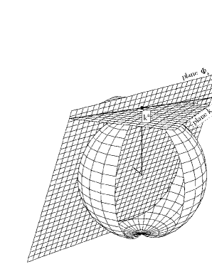
Figure 5: Relation between wave vector, electromagnetic field and the potential for the radiation gauge. In this gauge, the plane $\Phi_{a}$ is any plane intersecting the point $k^{a}$ on the wave sphere $\Omega^{ab}$, hinging around the line $F_{ab}$ which is the intersection between the plane $\Phi_{a}$ and the wave plane $k_{a}$.

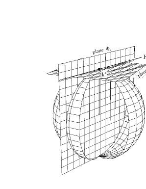
Figure 6: Relation between wave vector, electromagnetic field and the potential for the Coulomb gauge. In this gauge, $\Phi_{a}$ is the plane through the point $k^{a}$ and the center of the wave sphere $\Omega^{ab}$. The electromagnetic field is the same line of Fig. 5, the intersection between the plane $\Phi_{a}$ and the wave plane $k_{a}$.

namely that $\Phi_{a}$ is any plane that passes through the point of tangency of the wave plane $k_{a}$ with the wave sphere $\Omega^{ab}$ as shown in Fig. 5 (see (41) and following). The Coulomb gauge condition $\omega_{a}\Phi^{a}=0$ (106), however, imposes the condition that $\Phi_{a}$ passes through the center of the wave sphere $\omega_{a}\equiv(1,0,0,0)$. Taken together, these conditions imply that the plane $\Phi_{a}$ passes through the axis of the sphere normal to the wave plane $k_{a}$ (Fig. 6). The appropriateness of the projective interpretation is seen by noting that the significance of the line intersection of the planes $\Phi_{a}$ and $k_{a}$ is that it represents projectively the electromagnetic field tensor $F_{ab}$.

Let us suppose that the field tensor $F_{ab}$ is given. Algebraically, using homogeneous coordinates, $F_{ab}$ (102) in the Fourier domain is proportional to

$$F_{ab}\propto k_{a}\Phi_{b}-k_{b}\Phi_{a}$$ (119)

and it expresses the dual homogeneous coordinates of a line (56)-(58), called Pluecker coordinates in the projective space $\mathbb{P}^{3}$ [19].

Now, given the line $F_{ab}$ and the wavevector $k_{a}$ we have that $\Phi_{a}$ is a general plane in $\mathbb{P}^{3}$. Imposing the radiation gauge condition (105) we have that the plane $\Phi_{a}$ passes through the point $k^{a}$ but it has still the freedom to pivot about the line $F_{ab}$ (see Fig. 5). The unique representation is then obtained by choosing the one element of the family of planes $\Phi_{a}$ that passes through the center of the sphere, namely the plane which satisfy the Coulomb condition (106). Very nicely the geometry neatly illustrates the gauge freedom.

We now come to our main objective: to express the one index spinor $\psi_{A}$ geometrically. In the geometric interpretation, the totality of wave states with wave vector $k^{a}$ are obtained by the lines $F_{ab}$ that pass through the $k^{a}$ axis in the plane $k_{a}$. Note that we may admit complex lines as the geometry is generally valid over complex coordinates. For every line $F_{ab}$, the plane $\Phi_{a}$ is thus uniquely determined given the gauge fixing.

Now we consider the spinor equivalent of the plane $\Phi_{a}$ which is $\Phi_{AB^{\prime}}$ as in (103) still geometrically represented as a plane. As seen in the section II, spinors can be interpreted as complex lines generating the wave sphere (see equations (42)-(46)). We suppose that one of the two generators of the wave sphere $\bar{\theta}^{B^{\prime}}$ is chosen as a fixed reference generator. Then provided $\bar{\theta}^{B^{\prime}}$ does not lie in the plane $\Phi_{AB^{\prime}}$ (which is guaranteed by the gauge choice), there is a unique point of the generator $\bar{\theta}^{B^{\prime}}$ that intersects $\Phi_{AB^{\prime}}$ for any wave state and thus we can write

$$\psi_{A}=\Phi_{AB^{\prime}}\bar{\theta}^{B^{\prime}}.$$ (120)

The spinor $\psi_{A}$ represents the generator of the complementary family to $\bar{\theta}^{B^{\prime}}$ of the sphere that intersect $\Phi_{AB^{\prime}}$ in the same point as the $\bar{\theta}^{B^{\prime}}-$generator, since

• a linear relation must exist between these objects, due to the fact that generators of opposite type have a unique intersection. In fact, reconsidering the equation (120) we can rewrite it as

  $$\Phi_{AB^{\prime}}\psi^{A}\bar{\theta}^{B^{\prime}}=0,$$ (121)

  having contracted both sides of equation (120) with $\psi^{A}$ and using $\psi_{A}\psi^{A}=0$ as in (71). Now, if $\Phi_{AB^{\prime}}$ represents a plane, then $\psi^{A}\bar{\theta}^{B^{\prime}}$ represents a point $p^{a}$. This point is in general complex since the matrix obtained $P^{AB^{\prime}}=\psi^{A}\bar{\theta}^{B^{\prime}}$ is only singular but not necessarily Hermitian as in (37) or (II) and it is the intersection of the two generators (two lines) of the wave sphere of opposite families, $\psi^{A}$ and $\bar{\theta}^{B^{\prime}}$. Moreover, this point lies on the wave sphere since the matrix $P^{AB^{\prime}}$ is singular. Finally, the relation (121) tells us that that this null point belongs to the plane $\Phi_{AB^{\prime}}$.

• (120) is the only such relation that transforms covariantly and homogeneously.

Now, the reason we claim that we can identify the wave sphere with the Poincaré sphere is found by considering the effects of pure rotations about the $k^{a}$ axis for any wave state: it is seen that keeping $\bar{\theta}^{B^{\prime}}$ fixed when the plane $\Phi_{a}$ rotates by $180^{\circ}$, the same point of intersection arises. This explains the double rotation phenomenon of Stokes vectors, when rotation takes place around the wave vector. In fact we can construct the Stokes vector noting that only one point of any generator is real. It is clear that

$$\psi_{A}\bar{\psi}_{A^{\prime}}=\Psi_{AA^{\prime}}=\begin{pmatrix}\>\psi_{0}\bar{\psi}_{0^{\prime}}&\psi_{0}\bar{\psi}_{1^{\prime}}\\ \>\psi_{1}\bar{\psi}_{0^{\prime}}&\psi_{1}\bar{\psi}_{1^{\prime}}\\ \end{pmatrix}\;\rightarrow\;S_{a}$$ (122)

is a singular and Hermitian matrix (37) representing a coherency matrix for a single wave-state. It is isomorphic to a real vector $S_{a}$, the Stokes vector

$$S = (S_{0},S_{1},S_{2},S_{3})=$$

$$= (|\psi_{0}|^{2}+|\psi_{1}|^{2},2\,\mbox{Re}[\psi_{0}\bar{\psi}_{1^{\prime}}],-2\,\mbox{Im}[\psi_{0}\bar{\psi}_{1^{\prime}}],|\psi_{0}|^{2}-|\psi_{1}|^{2})$$

whose discriminating condition

$$S_{0}^{2}-S_{1}^{2}-S_{2}^{2}-S_{3}^{2}=0$$ (124)

recognizably represents a purely polarized state. Geometrically the vanishing of the determinant of $\Psi_{AA^{\prime}}$ expresses the condition that a plane should contain two conjugate generators ($\psi_{A}$ and $\bar{\psi}_{A^{\prime}}$) of the polarization sphere, so that the covariant Stokes vector $S_{a}$ represents a real tangent plane of the Poincaré sphere which now is fused with the wave sphere. In fact the condition (124) can be expressed as

$$S_{a}\Omega^{ab}S_{b}=0$$ (125)

which is the equation of a sphere in homogeneous coordinates (as in (44) and (43)).

We finally remark that $S$ is not a true tensor object because, like $\psi_{A}$ it omits structure (the phase flag essentially) that also has to transform geometrically.

The introduction of the phase flag is the key element to identify the polarization state for a wave vector in any direction with a spinor. Any transformation of geometric orientation does not change the spinor algebra. The spinor expression (120) transforms covariantly so that the relation will remain valid in any rotated frame if all the elements composing the relation are transformed with the appropriate rule as shown in (115)-(117). The essential distinction between geometric and polarimetric basis transformations is that in the former case the phase flag $\bar{\theta}^{B^{\prime}}$ must be transformed for consistency, while in the latter $\bar{\theta}^{B^{\prime}}$ must be regarded as fixed. Fixing $\bar{\theta}^{B^{\prime}}$ and varying $\Phi_{AB^{\prime}}$ we obtain all the polarization states for one direction of propagation.

VI Illustrative examples

We will now report some numerical examples in order to illustrate how all this really works.

We start first to choose one direction of propagation, which is as usual the $z-$direction. The covariant $4-$vector $k_{a}$ is then

$$k_{a}=k_{0}(1,0,0,-1)$$ (126)

with $k_{0}=\frac{\omega}{c}$. We choose now a linear polarized wave at $60^{\circ}$ to the $x-$axis propagating along $z$. The electromagnetic field tensor will be

$$F_{ab}=E\,\mbox{e}^{j(\omega t-\mathbf{k}\cdot\mathbf{x}+\alpha)}\begin{pmatrix}0&\quad\!\cos\frac{\pi}{3}&\quad\!\sin\frac{\pi}{3}&0\\ -\cos\frac{\pi}{3}&0&0&\cos\frac{\pi}{3}\\ -\sin\frac{\pi}{3}&0&0&\sin\frac{\pi}{3}\\ 0&-\cos\frac{\pi}{3}&-\sin\frac{\pi}{3}&0\\ \end{pmatrix}.$$ (127)

where $E$ is the amplitude of the wave, $\omega t-\mathbf{k}\cdot\mathbf{x}=\varphi$ is the phase (22) and $\alpha$ is an initial phase.

In order to isolate $\Phi_{a}$ from $F_{ab}$, we use the (102) contracting $F_{ab}$ with $t^{b}=(1,0,0,0)$. We obtain

$$F_{ab}t^{b}=j(k_{a}\Phi_{b}-k_{b}\Phi_{a})t^{b}\quad\Rightarrow\quad F_{a0}=-j\,k_{0}\,\Phi_{a}$$ (128)

and $\Phi_{a}$ has components

$$\Phi_{a}=\frac{j}{k_{0}}\,E\,\mbox{e}^{j(\varphi+\alpha)}\,\left(0,-\cos\frac{\pi}{3},-\sin\frac{\pi}{3},0\right).$$ (129)

Using (103), the corresponding $\Phi_{AB^{\prime}}$ is

$$\Phi_{AB^{\prime}}=\frac{j}{k_{0}}\,E\,\mbox{e}^{j(\varphi+\alpha)}\begin{pmatrix}0&-\cos\frac{\pi}{3}+j\sin\frac{\pi}{3}\\ -\cos\frac{\pi}{3}-j\sin\frac{\pi}{3}&0\\ \end{pmatrix}.$$ (130)

Now after selecting a convenient fixed generator $\theta^{B^{\prime}}$

$$\bar{\theta}^{B^{\prime}}=\frac{1}{\sqrt{2}}\begin{pmatrix}1\\ 1\\ \end{pmatrix},$$ (131)

we are ready to compute the polarization spinor $\psi_{A}$ with the (108):

$$\psi_{A} = jk_{0}\,\Phi_{AB^{\prime}}\bar{\theta}^{B^{\prime}}=jk_{0}\,(\Phi_{A0^{\prime}}\bar{\theta}^{0^{\prime}}+\Phi_{A1^{\prime}}\bar{\theta}^{1^{\prime}})=$$

$$= E\,\mbox{e}^{j(\varphi+\alpha)}\frac{1}{\sqrt{2}}\begin{pmatrix}\mbox{e}^{-j\frac{\pi}{3}}\\ \mbox{e}^{+j\frac{\pi}{3}}\\ \end{pmatrix},$$

which represents the Jones vector in circular polarization basis for a $60^{\circ}$ linear polarization. The corresponding polarization ratio is:

$$\mu=\mbox{e}^{j\frac{2\pi}{3}}.$$ (133)

We can calculate the corresponding Stokes vector using (V) and we obtain:

$$S_{a}=E^{2}\left(1,\cos\frac{2\pi}{3},\sin\frac{2\pi}{3},0\right).$$ (134)

which is the Stokes vector for a linear polarization with orientation angle $\psi=60^{\circ}$.

The next step is to see what changes if we choose another phase-flag $\bar{\theta}^{B^{\prime}}$, keeping in mind (112). For

$$\bar{\theta}^{B^{\prime}}=\frac{1}{\sqrt{2}}\begin{pmatrix}\mbox{e}^{-j\frac{\pi}{8}}\\ \mbox{e}^{j\frac{\pi}{8}}\\ \end{pmatrix},$$ (135)

we obtain

$$\psi_{A} = jk_{0}\,\Phi_{AB^{\prime}}\bar{\theta}^{B^{\prime}}=jk_{0}\,(\Phi_{A0^{\prime}}\bar{\theta}^{0^{\prime}}+\Phi_{A1^{\prime}}\bar{\theta}^{1^{\prime}})=$$

$$= E\,\mbox{e}^{j(\varphi+\alpha)}\frac{1}{\sqrt{2}}\begin{pmatrix}\mbox{e}^{-j(\frac{\pi}{3}-\frac{\pi}{8})}\\ \mbox{e}^{+j\frac{\pi}{3}-\frac{\pi}{8}}\\ \end{pmatrix}.$$

The corresponding polarization ratio and Stokes vector are

$$\mu=\mbox{e}^{2j(\frac{\pi}{3}-\frac{\pi}{8})}$$ (137)

$$S_{a}=E^{2}\left(1,\cos 2(\frac{\pi}{3}-\frac{\pi}{8}),\sin 2(\frac{\pi}{3}-\frac{\pi}{8}),0\right).$$ (138)

which is a linear polarization with orientation angle $\psi=15^{\circ}$. It is clear that the phase flag $\bar{\theta}^{B^{\prime}}$ keeps trace of the reference for the orientation angle of the polarization ellipse (see Fig. 4). We can notice that the components of the phase flag $\bar{\theta}^{B^{\prime}}$ apply phase factors to the circular polarization components as we have shown in (110). We can conclude that this phase offset is relative to the origin of the orientation angle. The phase flag is the element which defines the orientation angle and the phases of the circular polarization in a consistent manner. For these reasons it is the key to define polarization states for arbitrarily oriented wave vectors.

Now we can do the same calculation using the tensors instead of the spinors and for brevity we omit the multiplication constants. We have the plane $\Phi_{a}$. We calculate the Pluecker coordinates $\theta^{ab}$ of the line corresponding to the generator $\bar{\theta}^{B^{\prime}}$ and then the intersection of the plane potential with the line generator, in order to find the polarization state, the generator of the other type. We can use (46) where $\bar{\lambda}_{B^{\prime}}=\displaystyle{1\choose\lambda}$ and $\kappa_{A}=\displaystyle{1\choose\mu}$. We obtain:

$$\kappa_{A}\bar{\lambda}_{B^{\prime}}=\begin{pmatrix}1&\lambda\\ \mu&\mu\lambda\\ \end{pmatrix}=\begin{pmatrix}\tau-z&-x+jy\\ -x-jy&\tau+z\\ \end{pmatrix}.$$ (139)

Since we want to compute the generator through $\bar{\theta}^{B^{\prime}}$ then using (131) $\lambda=-1$. The corresponding one index tensor is:

$$t^{a}=(1-\mu,1-\mu,j+j\mu,-1-\mu).$$ (140)

In order to compute the projective Pluecker coordinates of this line, we consider two points on this line for example $p^{a}=(1,1,0,0)$ and $q^{a}=(0,0,j,-1)$, and we use the relations (49)-(51):

$$\theta^{\,ab}=\begin{pmatrix}0&0&j&-1\\ 0&0&j&-1\\ -j&-j&0&0\\ 1&1&0&0\\ \end{pmatrix},$$ (141)

$$(0,-j,1,0,1,j).$$ (142)

In order to find the generator of the other type, the polarization state, we compute the intersection of the line $\theta^{\,ab}$ with the plane $\Phi_{b}$:

$$\psi^{a}=\theta^{\,ab}\Phi_{b}=\left(\sin\frac{\pi}{3},\sin\frac{\pi}{3},-\cos\frac{\pi}{3},-j\cos\frac{\pi}{3}\right).$$ (143)

The spinor corresponding to this point will be computed using (139):

$$\mu=\frac{\tau+z}{-x+jy}=\mbox{e}^{2j\frac{\pi}{3}},$$ (144)

with of course $\tau=\sin\frac{\pi}{3}$, $x=\sin\frac{\pi}{3}$, $y=-\cos\frac{\pi}{3}$, $z=-j\cos\frac{\pi}{3}$. The spinor can be expressed as:

$$\psi_{A}\propto\begin{pmatrix}1\\ \mbox{e}^{j\frac{2\pi}{3}}\\ \end{pmatrix}$$ (145)

which is projectively the same as (VI).

Now we apply a rotation in space to the bivector $F^{ab}$, for example a rotation of $45^{\circ}$ about the $y-$axis. The rotation matrix turns out to be:

$$R^{\,a}_{\;\;b}=\begin{pmatrix}1&0&0&0\\ 0&\cos\frac{\pi}{4}&0&-\sin\frac{\pi}{4}\\ 0&0&1&0\\ 0&\sin\frac{\pi}{4}&0&\cos\frac{\pi}{4}\\ \end{pmatrix}.$$ (146)

The new electromagnetic field tensor will be:

$$\tilde{F}^{cd}=R^{\,c}_{\;\;a}R^{\,d}_{\;\;b}\,F^{ab}=$$ (147)

$$\begin{pmatrix}0&-\cos\frac{\pi}{4}\cos\frac{\pi}{3}&-\sin\frac{\pi}{3}&-\sin\frac{\pi}{4}\cos\frac{\pi}{3}\\ \cos\frac{\pi}{4}\cos\frac{\pi}{3}&0&\sin\frac{\pi}{4}\sin\frac{\pi}{3}&\cos\frac{\pi}{3}\\ \sin\frac{\pi}{3}&-\sin\frac{\pi}{4}\sin\frac{\pi}{3}&0&\cos\frac{\pi}{4}\sin\frac{\pi}{3}\\ \sin\frac{\pi}{4}\cos\frac{\pi}{3}&-\cos\frac{\pi}{3}&-\cos\frac{\pi}{4}\sin\frac{\pi}{3}&0\\ \end{pmatrix}.$$

We can notice that the equivalent matrix calculation to (147) would be:

$$\tilde{F}=RFR^{T}$$ (148)

where $F$, $\tilde{F}$ and $R$ indicate the corresponding matrices and $R^{T}$ is the transpose of the rotation matrix $R$.

The new wave vector will be:

$$\tilde{k}^{d}=R^{\,d}_{\;\;a}k^{a}=\left(1,-\sin\frac{\pi}{4},0,\cos\frac{\pi}{4}\right)$$ (149)

and

$$\tilde{k}_{a}=\left(1,\sin\frac{\pi}{4},0,-\cos\frac{\pi}{4}\right).$$ (150)

The new potential can be computed like in (128) and we obtain:

$$\tilde{\Phi}_{a}=\left(0,-j\cos\frac{\pi}{4}\cos\frac{\pi}{3},-j\sin\frac{\pi}{3},-j\sin\frac{\pi}{4}\cos\frac{\pi}{3}\right).$$ (151)

We can easily verify that the potential is still a plane through the origin $\omega^{a}$ and through the point $\tilde{k}^{a}$:

$$\tilde{\Phi}_{a}\omega^{a}=0,\quad\tilde{\Phi}_{a}\tilde{k}^{a}=0$$ (152)

In this calculation we are changing the orientation and calculating the corresponding new polarization state. In order to compute the new polarization state we have to rotate the generator $\theta^{ab}$ as well, to obtain:

$$\tilde{\theta}^{cd}=R^{\,c}_{\;\;a}R^{\,d}_{\;\;b}\,\theta^{ab}=\qquad\qquad\qquad\qquad\qquad\quad$$ (153)

$$=\begin{pmatrix}0&\sin\frac{\pi}{4}&j&-\cos\frac{\pi}{4}\\ -\sin\frac{\pi}{4}&0&j\cos\frac{\pi}{4}&-1\\ -j&-j\cos\frac{\pi}{4}&0&-j\sin\frac{\pi}{4}\\ \cos\frac{\pi}{4}&1&j\sin\frac{\pi}{4}&0\\ \end{pmatrix}.$$

In order to find the polarization state we need to find the point where the line $\tilde{\theta}^{cd}$ intersects the plane $\tilde{\Phi}_{a}$ as before.

$$\tilde{\psi}^{a}=\tilde{\theta}^{ab}\tilde{\Phi}_{b}=\left(\sin\frac{\pi}{3},j\cos\frac{\pi}{3}\sin\frac{\pi}{4}+\sin\frac{\pi}{3}\cos\frac{\pi}{4},\right.$$

$$\left.-\cos\frac{\pi}{3},-j\cos\frac{\pi}{3}\cos\frac{\pi}{4}+\sin\frac{\pi}{3}\sin\frac{\pi}{4}\right).$$ (154)

Using the definition (139) we can calculate the polarization ratios of the two generators:

$$\mu=\frac{\tau+z}{-x+jy}=\frac{\mbox{e}^{j\frac{2\pi}{3}}\cos\frac{\pi}{8}-\sin\frac{\pi}{8}}{\cos\frac{\pi}{8}+\mbox{e}^{j\frac{2\pi}{3}}\sin\frac{\pi}{8}},$$ (155)

$$\lambda=\frac{\tau+z}{-x-jy}=\frac{\cos\frac{\pi}{8}+\sin\frac{\pi}{8}}{-\cos\frac{\pi}{8}+\sin\frac{\pi}{8}}.$$ (156)

Now we perform the same calculation using spinors. We want to calculate the new polarization state for a new orientation $\tilde{k}^{a}$. It will be much faster and simpler. The unitary spinor corresponding to $R^{\,a}_{\;\;b}$ is $U^{\,A}_{\;\;B}$:

$$U^{\,A}_{\;\;B} = -\cos\frac{\pi}{8}\,\epsilon^{\,A}_{\;\;B}-j\sin\frac{\pi}{8}(\tau^{A}\omega_{B}+\omega^{A}\tau_{B})=$$ (157)

$$= \begin{pmatrix}\cos\frac{\pi}{8}&\sin\frac{\pi}{8}\\ -\sin\frac{\pi}{8}&\cos\frac{\pi}{8}\\ \end{pmatrix}$$

where

$$\tau^{A}=\frac{1}{\sqrt{2}}\begin{pmatrix}1\\ j\\ \end{pmatrix}\quad\omega^{A}=\frac{1}{\sqrt{2}}\begin{pmatrix}j\\ 1\\ \end{pmatrix}$$ (158)

are the spinor corresponding to the axis of rotation, the $y-$axis $T_{a}=(1,0,1,0)$ and the orthogonal one $O_{a}=(1,0,-1,0)$. $U^{\,A}_{\;\;B}$ represents the rotation in space the generates the new orientation $\tilde{k}^{a}$.

The new polarization spinor can be simply computed as

$$\tilde{\psi}^{A}=U^{\,A}_{\;\;B}\psi^{B}=\frac{j\,\mbox{e}^{-j\frac{\pi}{3}}}{\sqrt{2}}\begin{pmatrix}-\mbox{e}^{j\frac{2\pi}{3}}\cos\frac{\pi}{8}+\sin\frac{\pi}{8}\\ \cos\frac{\pi}{8}+\mbox{e}^{j\frac{2\pi}{3}}\sin\frac{\pi}{8}\\ \end{pmatrix}.$$ (159)

The corresponding covariant form of the spinor is:

$$\tilde{\psi}_{A}=\frac{j\,\mbox{e}^{-j\frac{\pi}{3}}}{\sqrt{2}}\begin{pmatrix}-\cos\frac{\pi}{8}-\mbox{e}^{j\frac{2\pi}{3}}\sin\frac{\pi}{8}\\ -\mbox{e}^{j\frac{2\pi}{3}}\cos\frac{\pi}{8}+\sin\frac{\pi}{8}\\ \end{pmatrix}$$ (160)

and the corresponding polarization ratio is exactly (155)

$$\mu=\frac{\mbox{e}^{j\frac{2\pi}{3}}\cos\frac{\pi}{8}-\sin\frac{\pi}{8}}{\cos\frac{\pi}{8}+\mbox{e}^{j\frac{2\pi}{3}}\sin\frac{\pi}{8}}.$$ (161)

The new phase flag $\bar{\tilde{\theta}}^{B^{\prime}}$ can be simply computed as

$$\bar{\tilde{\theta}}^{A^{\prime}}=\bar{U}^{\,A^{\prime}}_{\;\;B^{\prime}}\bar{\theta}^{B^{\prime}}=\frac{1}{\sqrt{2}}\begin{pmatrix}\cos\frac{\pi}{8}+\sin\frac{\pi}{8}\\ \cos\frac{\pi}{8}-\sin\frac{\pi}{8}\\ \end{pmatrix}.$$ (162)

Using the conjugate version of (68), the corresponding covariant phase flag is

$$\bar{\tilde{\theta}}_{B^{\prime}}=\epsilon_{A^{\prime}B^{\prime}}\bar{\tilde{\theta}}^{A^{\prime}}=\frac{1}{\sqrt{2}}\begin{pmatrix}-\cos\frac{\pi}{8}+\sin\frac{\pi}{8}\\ +\cos\frac{\pi}{8}+\sin\frac{\pi}{8}\\ \end{pmatrix}$$ (163)

and the corresponding polarization ratio is (156).

The corresponding Stokes vectors are

$$\tilde{\psi}^{A}\;\rightarrow\;\tilde{S}_{a}=\left(1,\cos\frac{2\pi}{3}\cos\frac{\pi}{4},\sin\frac{2\pi}{3},\cos\frac{2\pi}{3}\sin\frac{\pi}{4}\right),$$ (164)

$$\bar{\tilde{\theta}}^{B^{\prime}}\;\rightarrow\;\Theta_{b}=\left(1,-\cos\frac{\pi}{4},0,-\sin\frac{\pi}{4}\right).$$ (165)

$\tilde{\psi}^{A}$ is the new polarization state for a new orientation $\tilde{k}^{a}$ which corresponds to a new phase flag $\bar{\tilde{\theta}}^{B^{\prime}}$.

VII Discussion and conclusions

The representation that has been arrived at allows a spinor to describe a polarization state for a wave vector in any direction. In any fixed direction, we extend to Jones vector calculus in any chosen basis by applying unitary transformation to the polarization spinor alone, and not to the phase flag. The natural representation turns out, as might be expected, in terms of a circular polarization basis. If we change the direction of the wave vector we have also to apply the unitary transformation to the phase flag.

Geometrically this representation can be determined since two generators of the sphere $\psi_{A}$ and $\bar{\theta}^{B^{\prime}}$ (one of each kind) pass through any point of it, and then through every tangential plane representing a wave vector there pass two generators $\psi_{A}$ and $\bar{\psi}_{A^{\prime}}$ which are complex conjugates.

For the coherent field, one represents the polarization state of the propagating wave as

$$\psi_{A}\varpropto\mbox{e}^{jk_{a}x^{a}}=\mbox{e}^{j(\omega t-\mathbf{k}\cdot\mathbf{x})}$$ (166)

and the other, the conjugate field as

$$\bar{\psi}_{A^{\prime}}\varpropto\mbox{e}^{-jk_{a}x^{a}}=\mbox{e}^{j(-\omega t+\mathbf{k}\cdot\mathbf{x})}.$$ (167)

These fields are conjugate solutions, but both propagate in the same direction, as the equations for constant phase surface are identical. The use of strict spinor algebra prevents the often-committed error of associating a conjugated Jones vector with a backward propagating field. In each wave plane, therefore, there is one generator for the unconjugated Fourier component, and it is possible to show that the entire collection of these forms a ruled surface (regulus) on the wave sphere. The generator lying in the plane $(k_{0},\mathbf{k})$ corresponds to the wave state of $-1$ helicity (LHC), while the generator in the plane corresponding to the ’backward’ direction $(k_{0},-\mathbf{k})$ is that of $+1$ helicity (RHC).

This is the origin of the apparent conjugation/reversal symmetry. The lines on the regulus form a one-dimensional linear space, and in this sense we can say

$$\psi_{A}\equiv\begin{pmatrix}1\\ 0\\ \end{pmatrix}+\psi\begin{pmatrix}0\\ 1\\ \end{pmatrix}\quad\mbox{or}\quad\psi_{A}\equiv\psi_{0}\begin{pmatrix}1\\ 0\\ \end{pmatrix}+\psi_{1}\begin{pmatrix}0\\ 1\\ \end{pmatrix}$$ (168)

for a homogeneous projective spinor in which the complex polarization ratio $\psi=\frac{\psi_{1}}{\psi_{0}}$ runs from $0$ to $\infty$. As we have shown there is an isomorphism between the generators of the sphere and the set of the spinors $\psi_{A}$, and this can be effected in an invariant way with respect to any linear change of basis. Thus we have arrived at a unified polarimetric description in which both the geometry of ’world space’ and the abstract mapping of the generators of the sphere are handled consistently using spinors. The geometric interpretation we have introduced explains the fundamental place of the Poincaré sphere in polarimetry as an invariant object under linear transformations with its reguli whose generators are wave spinors, constituting its invariant subspaces. Identifying generators as states of polarization, the structure of the Poincaré sphere is preserved under all linear processes. The sphere is considered an invariant of the theory, the ’absolute quadric’ [19]. The Poincaré sphere and the wave sphere are hereby unified. The well-known phenomenon of ’double rotation’ of Stokes vectors with respect to rotation of world coordinates is down to the fact that $\bar{\theta}^{B^{\prime}}$ is not rotated when a basis transformation is made while for geometric transformations the phase flag is included (117). It may appear that the phase flag, $\bar{\theta}^{B^{\prime}}$ was introduced in a somewhat ad hoc manner, and indeed the choice

$$\bar{\theta}^{B^{\prime}}=\frac{1}{\sqrt{2}}\begin{pmatrix}1\\ 1\\ \end{pmatrix}$$ (169)

was not a unique one. It is obvious that the absolute phase of $\bar{\theta}^{B^{\prime}}$ could be chosen arbitrarily and even that its elements undergo relative phase transformation without loss of information. This is indeed the case, and so it appears wholly reasonable that we name this object the phase flag. Its practical importance is that it defines a phase reference for both components of the polarized wave. This is to be contrasted with conventions fixing one component as real, eg

$$\begin{pmatrix}\cos\theta\,\mbox{e}^{j\phi}\\ \sin\theta\\ \end{pmatrix},$$ (170)

which fails when $\theta\;\rightarrow\;\frac{\pi}{2}$. In a further planned paper on this topic we shall address the problems of defining the phase of an electromagnetic plane wave, and identifying the role of the phase flag in the relationship between geometry and phase.

David Bebbington Received the B.A. degree in experimental and theoretical physics and the Ph.D. degree in radio astronomy from Cambridge University, Cambridge, U.K., in 1977 and 1986, respectively. From 1981 to 1984, he worked on millimeter wave propagation research at the Rutherford Appleton Laboratory. Since 1984, he has been at the University of Essex, Essex, U.K., and currently holds the post of Senior Lecturer in the Department of Computing and Electronic System. His interests are polarimetry, applications of wave propagation in remote sensing, and weather radars.

Laura Carrea received the Laurea degree in physics from the University of Turin, Italy in 1997. From 1999 to 2004 she worked at the Faculty of Electrical Engineering and Information Technology at the Chemnitz University of Technology in Germany partly with a Fellowship in the frame of the Marie Curie TMR Network ”Radar Polarimetry: Theory and Application”. Since 2004 she is with Centre for Remote Sensing & Environmetrics, Department of Computing and Electronic System, University of Essex, U.K. Her main interests center on radar polarimetry.

Ernst Krogager received the M.Sc. degree in electrical engineering and the Danish technical doctor (Dr.Techn.) degree from the Technical University of Denmark, in 1981 and 1993, respectively. He has been an employee of the Danish Defence Research Establishment since 1981. Since 1984, he has conducted research in the areas of radar non-cooperative target identification and polarimetric radar imaging, and he has been the Danish representative in NATO working groups on the subject. From November 1989 until June 1990, he was temporarily with the Georgia Tech Research Institute, Atlanta, Georgia, USA, for studying radar polarimetry. During the fall of 1993, he conducted postdoctoral studies in radar polarimetry at the NASA Jet Propulsion Laboratory, Pasadena, California, USA. His primary research interests currently include the subject of High Power Microwaves.

TABLE I:

	The electromagnetic field
$\qquad F_{ab}=j(k_{a}\Phi_{b}-k_{b}\Phi_{a})\qquad$	$F_{ab}=\begin{pmatrix}\quad\!0&\quad\!E_{x}&\quad\!E_{y}&\quad\!0\\ -E_{x}&\quad\!0&\!0&\quad\!cB_{y}\\ -E_{y}&\quad\!0&\quad\!0&-cB_{x}\\ \!0&-cB_{y}&\quad\!cB_{x}&\quad\!0\\ \end{pmatrix}$
$\Bigg{\downarrow}\quad$ dropping the wave vector $k_{a}=(1,0,0,-1)$ information
	The electromagnetic potential
$\Phi_{a}=\frac{j}{k_{0}}F_{ab}t^{b}$	$\begin{array}[]{c}\Phi_{a}=\frac{j}{k_{0}}(0,-E_{x},-E_{y},0)\\ \Phi_{AB^{\prime}}=\frac{j}{k_{0}}\begin{pmatrix}0&-E_{x}+jE_{y}\\ -E_{x}-jE_{y}&0\\ \end{pmatrix}\\ \end{array}$
$\Bigg{\downarrow}\quad$ dropping the reference $\bar{\theta}^{B^{\prime}}=\displaystyle{1\choose 1}$ information
	The polarization spinor
$\psi_{A}=jk_{0}\Phi_{AB^{\prime}}\bar{\theta}^{B^{\prime}}$	$\psi_{A}=\begin{pmatrix}E_{x}-jE_{y}\\ E_{x}+jE_{y}\\ \end{pmatrix}$

Figure 4: An example where the same linear polarization is defined using two different phase flags. In one case we have used $\bar{\theta}^{B^{\prime}}=\textstyle{1\choose 1}$ which is the $x-$axes in circular basis. The orientation angle is $\psi=60^{\circ}$. In the other case we have used $\bar{\theta}^{B^{\prime}}=\textstyle{\;\mbox{e}^{-j\frac{\pi}{8}}\choose\;\mbox{e}^{+j\frac{\pi}{8}}}$ which is an axis of $45^{\circ}$ respect to the $x-$axis. The resulting orientation angle is $\psi=15^{\circ}$.

References

- [1] “http:www.dlr.detsxstart_en.htm.”
- [2] “http:www.dlr.dehrdesktopdefault.aspxtabid-23173669_read-5488.”
- [3] S. Cloude, “Ch. 2 - Lie groups in electromagnetic wave propagation and scattering,” in Electromagnetic Symmetry, C. Baum and H. Kritikos, Eds. Washington: Taylor and Francis, 1995, pp. 91–142.
- [4] J. Huynen, “Phenomenological theory of radar targets,” Ph.D. dissertation, Technical University of Delft, 1970.
- [5] R. Horn and C. Johnson, Matrix Analysis. Cambridge University Press, 1985.
- [6] E. Lüneburg, “Aspects of radar polarimetry,” Elektrik-Turkish Journal of Electrical Engineering and Computer Science, vol. 10, no.2, pp. 219–243, 2002.
- [7] H. Mott, Remote Sensing with Polarimetric Radar. John Wiley and Sons, 2007.
- [8] C. Graves, “Radar polarization power scattering matrix,” Proceedings of I.R.E., pp. 248–252, February 1956.
- [9] A. Kostinski and W.-M. Boerner, “On the foundations of radar polarimetry,” IEEE Trans. on Antenna and Propagation, vol. 34, pp. 1395–1404, 1986.
- [10] A. Agrawal and W.-M. Boerner, “Redevelopment of Kennaugh’s target characteristic polarization state theory using polarization transformation ratio formalism for the coherent case,” IEEE Trans. Geoscience and Remote Sensing, vol. 27, no.1, pp. 2–14, 1989.
- [11] J. Hubbert, “A comparison of radar, optics, and specular null polarization theory,” IEEE Trans. on Geoscience and Remote Sensing, vol. 32, no.3, pp. 658–671, 1994.
- [12] J. Hubbert and V. Bringi, “Specular null polarization theory: Applications to radar meteorology,” IEEE Trans. on Geoscience and Remote Sensing, vol. 34, no.4, pp. 859–873, 1996.
- [13] Z. Czyż, “Polarization and phase sphere of tangential phasors and its applications,” in Proc. SPIE Wideband Interferometric Sensing and Imaging Polarimetry, H. Mott and W. Boerner, Eds., vol. 3120, 1997, pp. 268–294.
- [14] H. Mieras, “Comments on ’On the foundations of radar polarimetry’, by A.B. Kostinski and W-M. Boerner,” IEEE Trans. on Antenna and Propagation, vol. 34, pp. 1470–1471, 1986.
- [15] A. Kostinski and W.-M. Boerner, “Reply to ’Comments on On the foundations of radar polarimetry’ by H. Mieras,” IEEE Trans. on Antenna and Propagation, vol. 34, pp. 1471–1473, 1986.
- [16] E. Lüneburg, “Comments on the ’Specular null polarization theory’, by J.C. Hubbert,” IEEE Trans. on Geoscience and Remote Sensing, vol. 35, no. 4, pp. 1070–1071, 1997.
- [17] J. Hubbert, “Reply to ’Comments on The specular null polarization theory’, by E. Lüneburg,” IEEE Trans. on Geoscience and Remote Sensing, vol. 35, no.4, pp. 1071–1072, 1997.
- [18] R. Azzam and N. Bashara, Ellipsometry and Polarized Light. Elsevier Science Pub Co, 1987.
- [19] J. Semple and G. Kneebone, Algebraic Projective Geometry. Oxford: Clarendon Press, 1952.
- [20] R. Jones, “A new calculus for the treatment of optical systems I: Description and discussion,” J. Opt. Soc. Am., vol. 31, pp. 488–493, 1941.
- [21] S. Cloude, “Polarimetric optimization based on the target covariance matrix,” Electronics Letters, vol. 26(20), pp. 1670–1671, 1990.
- [22] S. Cloude and E. Pottier, “A review of target decomposition theorems in radar polarimetry,” IEEE Trans. Geoscience and Remote Sensing, vol. 34, no.2, pp. 498–518, 1996.
- [23] D. Bebbington, E. Krogager, and M. Hellmann, “Vectorial generalization of target helicity,” in 3rd European Conference on Synthetic Aperture Radar (EuSAR), May 2000, pp. 531–534.
- [24] C. Misner, K. Thorne, and J. Wheeler, Gravitation. New York: W.H. Freeman and Company, 1973.
- [25] J.-C. Souyris and C. Tison, “Polarimetric analysis of bistatic SAR images from polar decomposition: a quaternion approach,” IEEE Trans. on Geoscience and Remote Sensing, vol. 45, no.9, pp. 2701–2714, 2007.
- [26] E. Corson, Introduction to Tensors, Spinors, and Relativistic Wave-Equations. London: Blackie & Son Ltd., 1954.
- [27] E. Cartan, The Theory of Spinors. Paris: Hermann, 1966.
- [28] R. Penrose, The Road to Reality. Vintage Books, 2006.
- [29] F. Perrin, “Polarization of light scattered by isotropic opalescent media,” J. Chem. Phys., vol. 10(7), pp. 415–427, 1942.
- [30] H. Ruse, “On the geometry of the electromagnetic field in general relativity,” Proc. London Math. Soc., vol. 41, no. 4, pp. 302–322, 1936.
- [31] H. Mott, Polarization in Antennas and Radar. John Wiley and Sons, 1986.
- [32] M. Nakahara, Geometry, Topology and Physics. Bristol and Philadelphia: Institute of Physics Publishing, 1990.
- [33] R. Penrose and W. Rindler, Spinors and Space-Time. Cambridge University Press, 1984, vol. 1.
- [34] J. Jackson, Classic Electrodynamics. John Wiley and Sons, 1999.
- [35] M. Tonnelat, The Principle of Electromagnetic Theory and of Relativity. Dordrecht, Holland: D. Reidel Publishing Company, 1966.
- [36] M. Born and E. Wolf, Priciples of Optics. Cambridge: Cambridge University Press, 1980.
- [37] J. Todd, Projective and Analytical Geometry. London: Sir Isaac Pitman & Sons, LTD, 1960.
- [38] M. Berger, Geometry II. Berlin, Heidelberg, New York: Springer Verlag, 1987.
- [39] B. van der Waerden, “Spinoranalyse,” Nachr. Akad. Wiss. Goetting. Math-Physik, vol. K1, pp. 100–109, 1929.
- [40] O. Laporte and G. E. Uhlenbeck, “Application of spinor analysis to the Maxwell and Dirac equations,” Phys. Rev., vol. 37, pp. 1380–1397, 1931.
- [41] H. Goldstein, Classical Mechanics. Reading, MA: Addison-Wesley, 1980.
- [42] D. Bebbington and M. Göbel, “KLEIN: a MATHEMATICA package for radar polarimetry based on spinor and tensor algebra,” Journal of Symbolic Computation, vol. 31, no. 6, pp. 745–751, 2001.
- [43] E. Post, Formal Structure of Electromagnetics - General Covariance and Electromagnetics. Dover Publications Inc., 1998.
- [44] M. Berry and S. Klein, “Geometric phases from stacks of crystal plates,” J. Mod. Optics, vol. 43, no. 1, pp. 165–180, 1996.
- [45] A. Ludwig, “The definition of cross polarization,” IEEE Trans. on Antenna and Propagation, vol. 21, pp. 116–119, 1973.
- [46] P. Boulanger and M. Hayes, Bivectors and Waves in Mechanics and Optics. Chapman and Hall, 1993.