Computation of the temperature dependence of the heat capacity of complex molecular systems using random color noise

Abstract

We propose a new method for computing the temperature dependence of the heat capacity in complex molecular systems. The proposed scheme is based on the use of the Langevin equation with low frequency color noise. We obtain the temperature dependence of the correlation time of random noises, which enables to model the partial thermalization of high-frequency vibrations, which is a pure quantum effect. By applying the method to carbon nanotubes, we show that the consideration of the color noise in the Langevin equation allows to reproduce the temperature evolution of the specific heat with good accuracy.

I Introduction

The pronounced temperature dependence of the specific heat $c(T)$ in molecular systems is a pure quantum effect. It is well known that in the absence of any critical point, the increase of the temperature is accompanied by a smooth rise of the specific heat $c(T)$, while by decreasing the temperature, $c(T)$ tends to zero. The first explanation for this phenomenon was given by Einstein a century ago en1 . This quantum effect results from the fact that at low temperatures, high frequency vibrations are partly frozen while low frequency vibrations are fully excited. It is of course impossible to explain the effect of partial thermalization within the framework of classical physics. In fact, the use of the usual Langevin equation with white noise leads to a uniform thermalization of all modes and the specific heat is practically insensitive to the temperature (in classical physics, any temperature dependence of the thermal capacity results from non-linearity effects). On the other hand, it is possible to mimic the partial thermalization effect in the framework of the Langevin description if one considers, instead of a white noise, a low frequency color noise with a temperature dependent frequency spectrum. To this end, it is enough to introduce a random noise with a finite correlation time $t_{c}>0$ during which the noise ”remembers”  its last realization. In this study, we obtain the temperature dependence of this correlation time, which allows a correct modeling of the partial thermalization of vibrations in the system.

The paper is organized as follows. We consider in Sec. I a harmonic oscillator and investigate its dynamics described by the Langevin equation with color noise. We obtain the temperature dependence of the correlation time of random noises, which enables us to efficiently model the partial thermalization of high-frequency vibrations. We next evaluate in Sec. II the effect of non-linearities on the accuracy of our computational method and propose a general scheme to compute the heat capacity for many-body systems using a color noise. The final section is devoted to the application of the proposed scheme to a Hamiltonian carbon nanotube model. It is shown in this section that the temperature evolution of the specific heat computed with the Langevin equation with color noise agrees well with the result obtained from a direct quantum mechanical calculation.

II The Langevin equation

The thermalization of the mode of frequency $\Omega$ is described by the Langevin equation

$$\ddot{u}+\Omega^{2}u+\Gamma\dot{u}=\xi(t)/\mu~{},$$ (1)

where $u$ is the coordinate of the vibration; damping $\Gamma=1/t_{r}$, and $t_{r}$ is the relaxation time; $\mu$ is the reduced mass of the mode; $\xi(t)$ is a normally distributed random force which describes the interaction of the mode with the thermal bath of temperature $T$ and the autocorrelation function

$$\langle\xi(t)\xi(t^{\prime})\rangle=2\mu\Gamma k_{B}T\varphi(t-t^{\prime})$$

(the dimensionless function $\varphi(t)$ is normalized as $\int_{-\infty}^{+\infty}\varphi(t)dt=1$), where $k_{B}$ is the Boltzmann constant.

At thermal equilibrium the averaged energy of thermal vibrations is defined by the relation

$$E=\lim_{\tau\rightarrow\infty}\frac{1}{\tau}\int_{0}^{\tau}\frac{\mu}{2}(\dot{u}^{2}+\Omega^{2}u^{2})dt$$

$$=\int_{0}^{+\infty}\mu(\omega^{2}+\Omega^{2})\left|H(\omega)\right|^{2}F(\omega)d\omega~{},$$ (2)

where $H(\omega)=\left[\mu(\Omega^{2}-\omega^{2}+i\omega\Gamma)\right]^{-1}$ is the transmission function and $F(\omega)$ is the Fourier transform of the autocorrelation function of the random force,

$$F(\omega)=\frac{1}{2\pi}\int_{-\infty}^{+\infty}\langle\xi(t)\xi(0)\rangle\exp\{-i\omega t\}dt$$

$$=\frac{\mu\Gamma k_{B}T}{\pi}\int_{-\infty}^{+\infty}\varphi(t)\exp\{-i\omega t\}dt~{}.$$ (3)

Thus, $E=K+P$ where the averaged kinetic energy is defined by the relation

$$K=\lim_{\tau\rightarrow\infty}\frac{1}{\tau}\int_{0}^{\tau}\frac{1}{2}\mu\dot{u}^{2}dt$$

$$=2k_{B}T\Gamma\int_{0}^{+\infty}\frac{\omega^{2}{\cal F}(\omega)d\omega}{(\Omega^{2}-\omega^{2})^{2}+\omega^{2}\Gamma^{2}}$$ (4)

and the averaged potential energy is given by

$$P=\lim_{\tau\rightarrow\infty}\frac{1}{\tau}\int_{0}^{\tau}\frac{1}{2}\mu\Omega^{2}u^{2}dt$$

$$=2k_{B}T\Gamma\int_{0}^{+\infty}\frac{\Omega^{2}{\cal F}(\omega)d\omega}{(\Omega^{2}-\omega^{2})^{2}+\omega^{2}\Gamma^{2}}~{},$$ (5)

where ${\cal F}(\omega)$ is the Fourier transform of the dimensionless autocorrelation function $\varphi(t)$:

$${\cal F}(\omega)=\frac{1}{2\pi}\int_{-\infty}^{+\infty}\varphi(t)\exp\{-i\omega t\}dt~{}.$$

For a delta-correlated random force (the case of the white noise), $\varphi(t)=\delta(t)$ and ${\cal F}(\omega)=1/2\pi$. The integrals (4) and (5) can be easily calculated by a contour integration. The energy $E=K=k_{B}T/2$ at $\Omega=0$ and $E=K+P=k_{B}T$, $K=P=k_{B}T/2$ for frequency $\Omega>0$.

For an exponentially-correlated random force (the case of low frequency color noise), $\varphi(t)=\frac{1}{2}\lambda\exp{-|\lambda t|}$ and ${\cal F}(\omega)=\lambda^{2}/2\pi(\omega^{2}+\lambda^{2})$, where $\lambda=1/t_{c}$ and $~{}t_{c}$ is the correlation time of the random force. In this case, the integrals (4) and (5) can also be calculated by a contour integration. The averaged kinetic energy $K=k_{B}Tf_{K}(\Omega,\Gamma,\lambda)/2$ and the averaged potential energy $P=k_{B}Tf_{P}(\Omega,\Gamma,\lambda)/2$ with $f_{K}$ and $f_{P}$ defined by

$$f_{K}(\Omega,\Gamma,\lambda) = \lambda^{2}/(\lambda^{2}+\lambda\Gamma+\Omega^{2})~{},$$ (6)

$$f_{P}(\Omega,\Gamma,\lambda) = \frac{\lambda^{2}(\Omega^{2}+\lambda^{2}-\Gamma^{2})+\lambda\Gamma\Omega^{2}}{(\Omega^{2}+\lambda^{2})^{2}-\Gamma^{2}\lambda^{2}}~{}.$$ (7)

In the case of an harmonic oscillator, the Langevin equation with white noise describes thermal vibrations of harmonic modes in the classical approximation, where the mean energy obeys $E=k_{B}T$. In the case of a quantum harmonic oscillator $H=\hbar\Omega(B^{+}B+\frac{1}{2})$, where $\hbar$ is the Planck constant, $B^{+}$ and $B$ represent creation and annihilation operators, the mean energy of thermal vibrations is given by

$$E(\Omega,T)=\frac{\hbar\Omega}{\exp(\hbar\Omega/k_{B}T)-1}+\frac{1}{2}\hbar\Omega~{}.$$ (8)

The heat capacity of the oscillator is defined by $c(\Omega,T)=dE(\Omega,T)/dT=k_{B}F_{E}(\Omega,T)$, where the Einstein function behaves according to

$$F_{E}(\Omega,T)=\left(\frac{\hbar\Omega}{k_{B}T}\right)^{2}\frac{\exp(\hbar\Omega/k_{B}T)}{[\exp(\hbar\Omega/k_{B}T)-1]^{2}}~{}.$$

For $T\rightarrow\infty$, the Einstein function $F_{E}(\Omega,T)\rightarrow 1$, while in the limit $T\rightarrow 0$, we get $F_{E}(\Omega,T)\rightarrow 0$. Consequently at high temperatures, the specific heat behaves as $c(\Omega,T)\approx k_{B}$ and at low temperatures, one has $c(\Omega,T)\approx 0$. For this reason, in the low temperature regime defined by $T<T_{E}=\hbar\Omega/k_{B}$, vibrations of the quantum oscillator are partially frozen. Consequently, a classical description of thermal vibrations is valid exclusively in the high temperature regime $T>T_{E}$, where the Einstein temperature $T_{E}$ is defined by $F_{E}(\Omega,T_{E})=e/(e-1)^{2}=0.9206735$ .

If we drop the energy of vacuum vibrations $\hbar\Omega/2$, the thermalization of the quantum oscillator can be characterized by the function

$$G(\Omega,T)=[E(\Omega,T)-\hbar\Omega/2]/k_{B}T$$

$$=\frac{\hbar\Omega/k_{B}T}{\exp(\hbar\Omega/k_{B}T)-1}~{}.$$

In the limit $T\rightarrow 0$, the thermalization coefficient $G(\Omega,T)\rightarrow 0$, while at $T=T_{E}$ the function $G(\Omega,T_{E})=1/(e-1)=0.5819767$, and in the limit $T\rightarrow\infty$, we have $~{}G(\Omega,T)\rightarrow 1$. Hence for temperatures $T>0$, vibrations with frequency $\Omega>\Omega_{E}(T)=k_{B}T/\hbar$ will be frozen. We can thus conclude that it is uncorrect to model thermal fluctuations of these modes using the Langevin equation with white noise.

As we stated at the beginning of this paper, the partial thermalization of high frequency vibrations and the total thermalization of low frequency modes can be realized if one uses a Langevin equation with color noise which consists of low frequency components of the white noise. But it is necessary to consider in this case the temperature dependence of the noise correlation functions. For an exponentially-correlated random noise, this dependence can be deduced from the relation

$$G(\Omega_{E}(T),T)\approx[f_{K}(\Omega_{E}(T),\Gamma,\lambda)+f_{P}(\Omega_{E}(T),\Gamma,\lambda)]/2.$$

In the limit $\Gamma\ll\Omega_{E}(T)=k_{B}T/\hbar$, using Eq. (6) and (7) the last equation can be expressed in the simple form

$$\frac{\lambda^{2}}{\lambda^{2}+(k_{B}T/\hbar)^{2}}=\frac{1}{e-1}~{}.$$ (9)

The equation (9) yields the following linear temperature dependence of the correlation coefficient :

$$\lambda=1/t_{c}=k_{B}T/\hbar\sqrt{e-2}~{}.$$ (10)

It follows from Eq. (10) that the description of the partial thermalization of high frequency vibrations with the use of the Langevin equation (1) becomes possible if we introduce a correlation time $t_{c}$ that is inversely proportional to the temperature $T$ of the thermal bath, i.e.

$$t_{c}=\hbar\sqrt{e-2}/k_{B}T~{}.$$ (11)

The time correlated color noise can be inserted in the Langevin description if one replaces the Langevin equation (1) by the system of two equations,

$$\ddot{u} = -\Omega^{2}u-\Gamma\dot{u}+\xi(t)/\mu,$$ (12)

$$\dot{\xi} = (\eta(t)-\xi(t))/t_{c},$$ (13)

where $\eta(t)$ stands for the white noise generator, normalized according to

$$\langle\eta(t)\eta(t^{\prime})\rangle=2\mu\Gamma k_{B}T\delta(t-t^{\prime}),$$

and $t_{c}$ is the correlation time whose temperature dependence is determined by (11).

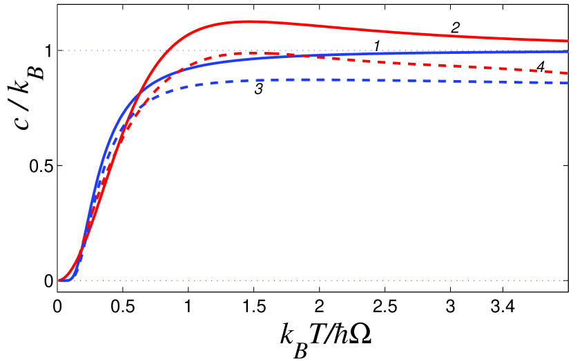
Figure 1: Temperature dependence of the heat capacity of the quantum harmonic (curve 1) and anharmonic oscillator (curve 3), classical harmonic (curve 2) and anharmonic oscillator (curve 4) obtained from the Langevin equation with color noise ($\Omega$ is the frequency of the oscillator and the anharmonicity parameter is chosen as $\beta=0.1$).

Fig. 1 compares the specific heat of a quantum harmonic oscillator and a classical oscillator whose dynamics is described by Langevin equations with color noise (12) and (13). It is clear that the introduction of the color noise doesn’t allow to reproduce the temperature dependence of the quantum oscillator exactly. This is mainly due to the well known inadequacy of a classical description to describe zero vibrations (ground state fluctuations). The figure nevertheless shows that the use of the color noise yields a qualitatively correct behaviour of the heat capacity, that is, in the limit $T\rightarrow 0$ the specific heat $c\rightarrow 0$, and for $T\rightarrow\infty$ one has $c\rightarrow k_{B}$ (with the increase of the temperature, the correlation time tends to zero and the color noise becomes a white noise). Most importantly, we notice that there is a good agreement between the exact quantum result and the modified Langevin description at low temperatures $T<T_{E}$ where quantum effects dominate.

We have shown that by using the Langevin equation with color noise, one can obtain a qualitatively correct picture for the temperature evolution of the specific heat in the case of a harmonic oscillator. The presence of non-linearities in the system will be tackled in the next section.

III The efficiency of the proposed scheme in the presence of non-linearities

As is well-known, anharmonicities are always present in physical systems and the validity of the harmonic approximation which consists in representing the building blocks of a condensed system by linear oscillators is usually restricted to very low energy regimes. The anharmonic intermolecular forces may result either from the non-linearity of the individual oscillators or from their non-linear mutual interaction. The natural question arises whether the Langevin equation with color noise can be used in the presence of non-linearities in the system. As a first attempt to answer this question, let us consider a non-linear oscillator whose dimensionless Hamiltonian is given by

$$H=\frac{1}{2}\dot{u}^{2}+\frac{1}{2}u^{2}+\frac{1}{4}\beta u^{4}~{}.$$ (14)

The corresponding Langevin equation with color noise can be written in the form

$$\ddot{u} = -u-\beta u^{3}-\Gamma\dot{u}+\xi(t),$$

$$\dot{\xi} = (\eta(t)-\xi(t))/t_{c},$$

$$\langle\eta(t)\eta(t^{\prime})\rangle=2\Gamma T\delta(t-t^{\prime}),$$

where $T$ - the dimensionless temperature, the friction coefficient $\Gamma=0.01$ and the correlation time $t_{c}=\sqrt{e-2}/T$.

The numerical integration of the set of equations of motion (III) yields the mean energy $E=\langle H\rangle$ of the anharmonic oscillator as a function of $T$. Then the specific heat is computed from $c(T)=dE/dT$.

In order to check the accuracy of the modified Langevin equation, we equally obtained the specific heat of this oscillator by computing numerically the exact eigenvalues $E_{n}$ of the quartic Hamiltonian (14). The diagonalization of the hamiltonian matrix was performed in the basis of the harmonic oscillator. The obtained eigenvalues were then used to find the partition function and the specific heat from the well-known relations

$$Z(T) = \sum_{n}e^{-E_{n}/T},$$

$$F(T) = -T\ln(Z),$$ (16)

$$c(T) = -T\frac{d^{2}F}{dT^{2}}.$$

We compare in Fig. 1 the result of the numerical simulation to that obtained from the quantum statistical calculation (curve 3 and 4) at $\beta=0.1$. We notice that the non-linearity effects are indistinguishable within the accuracy of the proposed method.

Let us note that Kleinert‘s variational path integral method allows us to obtain a fully analytical expression for the specific heat of this quantum oscillator Kleinert . The method aims at approximating the quantum partition function

$$Z=\int\mathbf{\emph{D}x}\hskip 1.42262pte^{-S[\mathbf{x}]},$$ (17)

where

$$S=\int d\tau\left(\frac{m}{2}\dot{\mathbf{x}}^{2}+V[\mathbf{x}]\right)$$ (18)

is the Euclidean action, with a quadratic trial action $S_{0}[\mathbf{x}]$ whose variational parameters are fixed by minimizing the right hand sight of the Jensen-Peirels inequality,

$$F\leq F_{0}+T\left<S-S_{0}\right>.$$ (19)

This first order perturbation theory allows to compute the approximative quantum partition function of a $N$-body system as an integration over the classical configurational space,

$$Z=\int\frac{d\mathbf{x_{0}}}{\left(2\pi/T\right)^{N/2}}e^{-W(\mathbf{x_{0}})/T}.$$ (20)

where $W(\mathbf{x_{0}})$ is the so-called centroid potential and $x_{0}$ stands for the centroid path Kleinert ; Tognetti .

The effective potential $W(x_{0})$ obtained by Kleinert for the trivial case of the quartic oscillator Kleinert is given in the appendix. We verified that for $\beta=0.1$, the analytical expression of the specific heat obtained from the partition function (20) reproduces the numerical result (curve 3) of Fig. 1 with an error that is imperceptible on this scale.

In order to examine the effect of non-linearities present in mutual interactions between vibrational modes, let us consider now the case of two linear oscillators with a dimensionless Hamiltonian

$$H=\frac{1}{2}(\dot{u}_{1}^{2}+\dot{u}_{2}^{2}+\omega_{1}^{2}u_{1}^{2}+\omega_{2}^{2}u_{2}^{2})+\frac{1}{4}\beta(u_{1}-u_{2})^{4},$$ (21)

where the variable $u_{i}$ describes the dynamics of the $i$-th oscillator $(i=1,2)$, $\omega_{i}$ the frequency of the same mode, and the parameter $\beta$ sets the strength of the non-linear interaction between the two oscillators. For this two-body hamiltonian, the system of Langevin equations with color noise takes the form

$$\ddot{u_{1}} = -\omega_{1}u_{1}+\beta(u_{2}-u_{1})^{3}-\Gamma\dot{u_{1}}+\xi_{1}(t),$$

$$\ddot{u_{2}} = -\omega_{2}u_{2}-\beta(u_{2}-u_{1})^{3}-\Gamma\dot{u_{2}}+\xi_{2}(t),$$ (22)

$$\dot{\xi_{1}} = (\eta_{1}(t)-\xi_{1}(t))/t_{c},$$

$$\dot{\xi_{2}} = (\eta_{2}(t)-\xi_{2}(t))/t_{c},$$

where $\eta_{i}(t)$ stands for the random function that generates white noise with normalization conditions

$$\langle\eta_{i}(t)\eta_{i}(t^{\prime})\rangle=2\Gamma T\delta(t-t^{\prime}),~{}~{}i=1,2,~{}~{}\langle\eta_{1}(t)\eta_{2}(t^{\prime})\rangle=0.$$

($T$ - dimensionless temperature, the dissipation coefficient is chosen as $\Gamma=0.01$, and the correlation time is given by $t_{c}=\sqrt{e-2}/T$).

It is also possible for this two-body system to obtain the temperature dependence of the specific heat from a purely quantum mechanical calculation, that is, by diagonalizing the hamiltonian matrix corresponding to Eq. (21) in the product basis of two harmonic oscillators of frequencies $\omega_{1}$ and $\omega_{2}$. The obtained energy levels were then used in Eq. (16) in order to obtain the specific heat.

For the sake of distinctness, we chose $\omega_{1}=1$ and $\omega_{2}=10$. The result of the numerical integration of the equations of motion (22) illustrated in Fig. 2 indeed shows that the presence of non-linearities in the interaction between individual modes improves the precision of the proposed Langevin approach with color noise. To be more precise, for an interaction strength of $\beta=1$, the temperature dependence of $c(T)$ agrees better than the non-interacting case $\beta=0$ with the result obtained from quantum statistical mechanics.

Using once more Kleinert‘s variational path integral method, we derived an analytical expression for the partition function of the two-body Hamiltonian (21). The calculation is summarized in the appendix and the analytical result agrees very well with the numerical result in the temperature regime $T>0.3$.

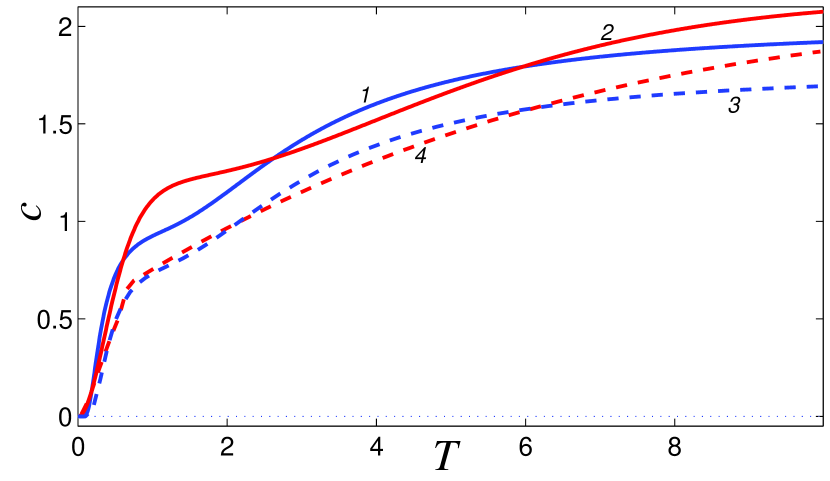
Figure 2: Temperature dependence of the heat capacity for the system of two coupled linear oscillators (with frequencies $\omega_{1}=1$, $\omega_{2}=10$) obtained from a direct quantum mechanical calculation (curves 1, 3) and the Langevin equation with color noise (curves 2, 4). Solid lines correspond to decoupled oscillators ($\beta=0$) and dashed lines to a coupling $\beta=1$.

These two examples clearly shows that the use of the Langevin equation with color noise can be used as a reasonably accurate tool to compute the specific heat of complex molecular systems that are very difficult to study within the framework of quantum statistical mechanics.

We will now present the scheme for evaluating the temperature dependence of the specific heat for general molecular systems by using a color noise. Let us define the $N$ dimensional vector ${\bf x}=\{x_{n}\}_{n=1}^{N}$ which denotes the spatial coordinates of the individual atoms in the system. In terms of these coordinates, the generalized Langevin equation describing the dynamics of the system takes the form

$${\bf M}\ddot{\bf x} = -\partial H/\partial{\bf x}-\Gamma{\bf M}\dot{\bf x}+\Xi,$$ (23)

$$\dot{\Xi} = (\Theta-\Xi)/t_{c},$$ (24)

where ${\bf M}$ - the mass matrix of the atoms, $H$ - the Hamiltonian of the system, the dissipation coefficient is given by $\Gamma=1/t_{r}$ ($t_{r}$ - the relaxation time), $\Theta=\{\eta_{n}\}_{n=1}^{N}$ is the vector of normally distributed random forces obeying the normalization conditions

$$\langle\eta_{n}(t_{1})\eta_{l}(t_{2})\rangle=2M_{n}k_{B}T\delta_{nl}\delta(t_{1}-t_{2}),$$ (25)

and the temperature dependence of the correlation time $t_{c}$ is still determined by the relation (11). The choice of characteristic times for the integration of the generalized Langevin equations requires some care. In fact, since the formula (11) was obtained in the limit $\Gamma\gg k_{B}T/\hbar$, the numerical value of the relaxation time should be large enough. It is thus crucial that the fixed value of the relaxation time remains always bigger than the correlation time of random forces in the considered temperature regime. On the other hand, very large values of $t_{r}$ are not suitable since it would require exceedingly long integration times to drive the system to thermal equilibrium. From a practical point of view, the numerical value $t_{r}=1$ ps is adequate since the result remains practically invariant under the increase of this characteristic time.

The proposed scheme will be applied in the next section to a Hamiltonian carbon nanotube model.

IV Computation of the heat capacity of carbon nanotubes

Carbon nanotubes have the peculiarity of behaving as quasi-one-dimensional systems. This characteristic allows us to compute the specific heat of these structures using quantum statistical tools and this is what we will exploit in this section in order to check the efficiency of our modified Langevin approach on a concrete molecular system.

For the sake of simplicity we will limit ourselves to the case of a nanotube with index of chirality $(m,m)$. The structure of a carbon nanotube (CNT) with chirality $(m,m)$ (armchair structure) is shown schematically in Fig. 3. The nanotube is characterized by its radius $R$, the angle shift $\varphi$ and the longitudinal step $h$. The system consists of parallel transversal layers of atoms. In each layer, the nanotube has $2m$ atoms, which form $m$ elementary cells separated by the angular distance $\Delta\phi=2\pi/m$, so that $h$ defines alternating longitudinal distances between the transverse layers. Each atom of the CNT can be characterized by three indices $(n,l,k)$, where $(n,l)$ defines an elementary cell ($n=0,\pm 1,\ldots$, $l=1,2,\ldots,m$), and $k$ is the atom number in the cell, $k=0,1$ (see Fig. 3).

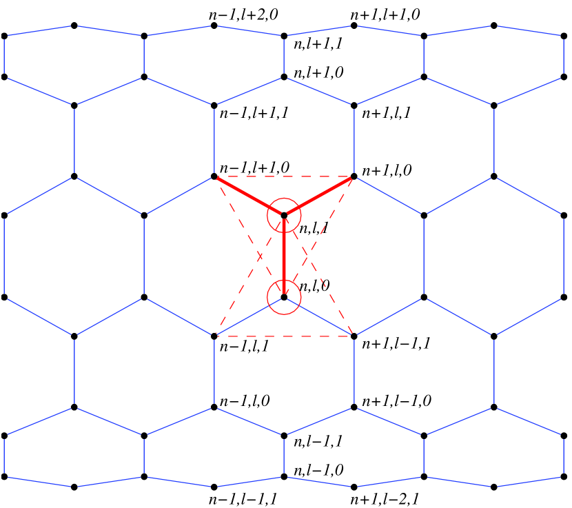
Figure 3: Schematic representation of a carbon nanotube with chirality $(m,m)$ and numbering of atoms in the structure. Thick red lines mark valent bond couplings, thin red arcs marks valent angle couplings, thin dashed lines show the foundation of two pyramids which form dihedral angles along the valent bonds in the elementary cell $(n,l)$. For this figure, we chose $m=6$.

The Hamiltonian of the lattice of carbon atoms shown in Fig. 3 can be written in the following general form,

$${\cal H}=\sum_{n}\sum_{l=1}^{m}\biggr{[}\frac{1}{2}M(\dot{\bf u}^{2}_{n,l,0}+\dot{\bf u}^{2}_{n,l,1})+{\cal P}_{n,l}\}\biggr{]}$$ (26)

where $M$ is the mass of a carbon atom, $M=12\times 1.6603\cdot 10^{-27}$kg, ${\bf u}_{n,l,k}=(x_{n,l,k}(t),y_{n,l,k}(t),z_{n,l,k}(t))$ is the radius-vector that defines the position of the carbon atom $(n,l,k)$ in the moment $t$, and the term ${\cal P}_{n,l}\equiv P({\bf u}_{n-1,l,1},{\bf u}_{n-1,l+1,0},{\bf u}_{n,l,0},{\bf u}_{n,l,1},{\bf u}_{n+1,l-1,1},{\bf u}_{n+1,l,0})$ denotes the total potential energy given by a sum of three different types of potentials,

$${\cal P}_{n,l}=V({\bf u}_{n,l,0},{\bf u}_{n,l,1})+V({\bf u}_{n-1,l+1,0},{\bf u}_{n,l,1})+V({\bf u}_{n,l,1},{\bf u}_{n+1,l,0})+U({\bf u}_{n-1,l,1},{\bf u}_{n,l,0},{\bf u}_{n,l,1})$$

$$+ U({\bf u}_{n+1,l-1,1},{\bf u}_{n,l,0},{\bf u}_{n,l,1})+U({\bf u}_{n-1,l,1},{\bf u}_{n,l,0},{\bf u}_{n+1,l-1,1})+U({\bf u}_{n,l,0},{\bf u}_{n,l,1},{\bf u}_{n-1,l+1,0})$$

$$+ U({\bf u}_{n,l,0},{\bf u}_{n,l,1},{\bf u}_{n+1,l,0})+U({\bf u}_{n-1,l+1,0},{\bf u}_{n,l,1},{\bf u}_{n+1,l,0})+W({\bf u}_{n,l,1},{\bf u}_{n,l,0},{\bf u}_{n-1,l,1},{\bf u}_{n+1,l-1,1})$$

$$+ W({\bf u}_{n,l,1},{\bf u}_{n,l,0},{\bf u}_{n+1,l-1,1},{\bf u}_{n-1,l,1})+W({\bf u}_{n-1,l,1},{\bf u}_{n,l,0},{\bf u}_{n,l,1},{\bf u}_{n+1,l-1,1})+W({\bf u}_{n,l,0},{\bf u}_{n,l,1},{\bf u}_{n-1,l+1,0},{\bf u}_{n+1,l,0})$$

$$+ W({\bf u}_{n,l,0},{\bf u}_{n,l,1},{\bf u}_{n+1,l,0},{\bf u}_{n-1,l+1,0})+W({\bf u}_{n-1,l+1,0},{\bf u}_{n,l,1},{\bf u}_{n,l,0},{\bf u}_{n+1,l,0}).$$

The first three terms describe a change of the deformation energy due to a direct interaction between pairs of atoms with coordinates ${\bf u}_{1}$ and ${\bf u}_{2}$, characterized by the potential $V({\bf u}_{1},{\bf u}_{2})$. The next six terms describe the deformation energy of the angle between the links ${\bf u}_{1}{\bf u}_{2}$ and ${\bf u}_{2}{\bf u}_{3}$, taken into account with the potential $U({\bf u}_{1},{\bf u}_{2},{\bf u}_{3})$. Finally, the next six terms describe the deformation energy associated with a change of the effective angle between the planes ${\bf u}_{1}{\bf u}_{2}{\bf u}_{3}$ and ${\bf u}_{2}{\bf u}_{3}{\bf u}_{4}$, characterized by the potential $W({\bf u}_{1},{\bf u}_{2},{\bf u}_{3},{\bf u}_{4})$.

In our numerical simulations, we employ the interaction potentials frequently used in modeling of the dynamics of polymer macromolecules p1 ; p2 ; p3 ,

$$V({\bf u}_{1},{\bf u}_{2})=D\{\exp[-\alpha(\rho-\rho_{0})]-1\}^{2},$$ (28)

where $\rho=|{\bf u}_{2}-{\bf u}_{1}|$, $D=4.9632$ eV is the energy of the valent coupling, and $\rho_{0}=1.418$Å is the static length of valent bond;

$$U({\bf u}_{1},{\bf u}_{2},{\bf u}_{3})=\epsilon_{v}(\cos\varphi-\cos\varphi_{0})^{2},$$ (29)

where

$$\cos\varphi=({\bf u}_{3}-{\bf u}_{2},{\bf u}_{1}-{\bf u}_{2})(|{\bf u}_{3}-{\bf u}_{2}|\cdot|{\bf u}_{2}-{\bf u}_{1}|)^{-1},$$

and $\cos\phi_{0}=\cos(2\pi/3)=-1/2$. Finally,

$$W({\bf u}_{1},{\bf u}_{2},{\bf u}_{3},{\bf u}_{4})=\epsilon_{t}\left[1-({\bf v}_{1},{\bf v}_{2})(|{\bf v}_{1}|\cdot|{\bf v}_{2}|)^{-1}\right],$$ (30)

where ${\bf v}_{1}=({\bf u}_{2}-{\bf u}_{1})\times({\bf u}_{3}-{\bf u}_{2})$ and ${\bf v}_{2}=({\bf u}_{3}-{\bf u}_{2})\times({\bf u}_{4}-{\bf u}_{3})$. The model parameters such as $\alpha=1.7889$ Å^-1, $\epsilon_{v}=1.3143$ eV, and $\epsilon_{t}=0.499$ eV can be determined from the phonon frequency spectrum of a planar lattice of carbon atoms p16 ; pai .

Equilibrium structure of the nanotube with index $(m,m)$ can be characterized by three parameters : its radius $R$, the angle shift $\varphi$ and the longitudinal step $h$. Equilibrium positions of the atoms in the tube are given by the coordinates

$$x^{0}_{n,l,0}=h(n-1)$$, ,

, ,

, ,

(31)

with cylindrical angles $\phi_{n,l}=[l-1+(n-1)/2]\Delta\phi$ and the angular distance $\Delta\phi=2\pi/m$. In order to find the parameters $R$, $\varphi$ and $h$, we need to solve the minimization problem

$$P({\bf u}_{n-1,l,1}^{0},{\bf u}_{n-1,l+1,0}^{0},{\bf u}_{n,l,0}^{0},{\bf u}_{n,l,1}^{0},{\bf u}_{n+1,l-1,1},{\bf u}_{n+1,l,0}^{0})$$

$$\rightarrow\min_{R,\varphi,h},$$

where we have introduced the notations ${\bf u}_{n,l,i}^{0}=(x_{n,l,i}^{0},y_{n,l,i}^{0},z_{n,l,i}^{0})$ and $i=0,1$. The resulting value of the energy is then used as the minimum value. For a nanotube of the (6,6) type, we find a radius $R=4.1782$ Å and a longitudinal step $h=1.2590$ Å while for a nanotube of the (12,12) type, one obtains $R=8.3230$ Å and $h=1.2560$ Å.

If one wishes to study small amplitude vibrations, it is more convenient to switch to local cylindrical coordinates $u_{n,l,k}$, $v_{n,l,k}$, $w_{n,l,k}$ defined by

$$x_{n,l,k} = x_{n,l,k}^{0}+u_{n,l,k},$$

$$y_{n,l,k} = y_{n,l,k}^{0}-v_{n,l,k}\sin\phi_{n,l,k}^{0}+w_{n,l,k}\cos\phi_{n,l,k}^{0},~{}~{}~{}~{}$$ (32)

$$z_{n,l,k} = z_{n,l,k}^{0}+v_{n,l,k}\cos\phi_{n,l,k}^{0}+w_{n,l,k}\sin\phi_{n,l,k}^{0},$$

with the angle $\phi_{n,l,0}=[l-1+(n-1)/2]\Delta\phi$ and $\phi_{n,l,1}=\phi_{n,l,0}+\varphi$. In this coordinate system, the Hamiltonian of the carbon nanotube takes the form

$${\cal H}=\sum_{n}\sum_{l=1}^{m}\{\frac{1}{2}M(\dot{\bf x}_{n,l},\dot{\bf x}_{n,l})+P({\bf x}_{n-1,l};{\bf x}_{n-1,l+1};{\bf x}_{n,l};{\bf x}_{n+1,l-1};{\bf x}_{n+1,l})\},$$ (33)

where the six dimensional vector ${\bf x}_{n,l}=(u_{n,l,0},v_{n,l,0},w_{n,l,0},u_{n,l,1},v_{n,l,1},w_{n,l,1})$ describes in local coordinates the shifting of the atoms located in the cell $n,l$ from their equilibrium position.

The equations of motion for the Hamiltonian (33) are given by

$$-M\ddot{\bf x}_{n,l} = -{\bf F}_{n,l}=P_{{\bf x}_{1}}({\bf x}_{n,l};{\bf x}_{n,l+1};{\bf x}_{n+1,l};{\bf x}_{n+2,l-1};{\bf x}_{n+2,l})+P_{{\bf x}_{2}}({\bf x}_{n,l-1};{\bf x}_{n,l};{\bf x}_{n+1,l-1};{\bf x}_{n+2,l-2};{\bf x}_{n+2,l-1})$$

$$+ P_{{\bf x}_{3}}({\bf x}_{n-1,l};{\bf x}_{n-1,l+1};{\bf x}_{n,l};{\bf x}_{n+1,l-1};{\bf x}_{n+1,l})+P_{{\bf x}_{4}}({\bf x}_{n-2,l+1};{\bf x}_{n-2,l+2};{\bf x}_{n-1,l+1};{\bf x}_{n,l};{\bf x}_{n,l+1})$$

$$+ P_{{\bf x}_{5}}({\bf x}_{n-2,l};{\bf x}_{n-2,l+1};{\bf x}_{n-1,l};{\bf x}_{n,l-1};{\bf x}_{n,l}),$$

with the function $P_{{\bf x}_{i}}=\frac{\partial}{\partial{\bf x}_{i}}P({\bf x}_{1},{\bf x}_{2},{\bf x}_{3},{\bf x}_{4},{\bf x}_{5})$, $i=1,2,...,5$. In the linear approximation, the same set of equations takes the form

$$-M\ddot{\bf x}_{n,l} = B_{1}{\bf x}_{n,l}+B_{2}{\bf x}_{n+1,l}+B_{2}^{*}{\bf x}_{n-1,l}+B_{3}{\bf x}_{n+2,l}+B_{3}^{*}{\bf x}_{n-2,l}+B_{4}{\bf x}_{n,l+1}+B_{4}^{*}{\bf x}_{n,l-1}$$ (35)

$$+ B_{5}{\bf x}_{n+1,l-1}+B_{5}^{*}{\bf x}_{n-1,l+1}+B_{6}{\bf x}_{n+2,l-1}+B_{6}^{*}{\bf x}_{n-2,l+1}+B_{7}{\bf x}_{n+2,l-2}+B_{7}^{*}{\bf x}_{n-2,l+2},$$

where the matrix coefficients are defined as

$$B_{1}=P_{{\bf x}_{1}{\bf x}_{1}}+P_{{\bf x}_{2}{\bf x}_{2}}+P_{{\bf x}_{3}{\bf x}_{3}}+P_{{\bf x}_{4}{\bf x}_{4}}+P_{{\bf x}_{5}{\bf x}_{5}},~{}~{}~{}B_{2}=P_{{\bf x}_{1}{\bf x}_{3}}+P_{{\bf x}_{3}{\bf x}_{5}},~{}~{}~{}B_{3}=P_{{\bf x}_{1}{\bf x}_{5}},$$

$$B_{4}=P_{{\bf x}_{1}{\bf x}_{2}}+P_{{\bf x}_{4}{\bf x}_{5}},~{}~{}~{}B_{5}=P_{{\bf x}_{2}{\bf x}_{3}}+P_{{\bf x}_{3}{\bf x}_{4}},~{}~{}~{}B_{6}=P_{{\bf x}_{1}{\bf x}_{4}}+P_{{\bf x}_{2}{\bf x}_{5}},~{}~{}~{}B_{7}=P_{{\bf x}_{2}{\bf x}_{4}},$$

with the matrix of partial derivatives

$$P_{{\bf x}_{i},{\bf x}j}=\frac{\partial^{2}P}{\partial{\bf x}_{i}\partial{\bf x}_{j}}({\bf 0},{\bf 0},{\bf 0},{\bf 0},{\bf 0}),~{}~{}~{}i,j=1,2,3,4,5~{}.$$

The solution of the linearized equations (35) can be found in terms of plane waves in the form

$${\bf x}_{nl}=A{\bf e}\exp(iqn+il\delta\phi-i\omega t),$$ (36)

where $A$ stands for the amplitude of the wave, $\bf e$ - the unit vector of the amplitude, $q\in[0,\pi]$ - the dimensionless wave number and $\delta=2\pi j/m$ ($j=0,1,...,m-1$) – the dimensionless orbital moment of the phonon. By injecting the expression (36) into the linear equation system (35), we obtain the eigenvalue problem

$$M\omega^{2}{\bf A}=[B_{1}+B_{2}e^{iq}+B_{2}^{*}e^{-iq}+B_{3}e^{2iq}+B_{3}^{*}e^{-2iq}+B_{4}e^{i\delta}+B_{4}^{*}e^{-i\delta}~{}~{}~{}~{}$$

$$+B_{5}e^{iq-i\delta}+B_{5}^{*}e^{-iq+i\delta}+B_{6}e^{2iq-i\delta}+B_{6}^{*}e^{-2iq+i\delta}+B_{7}e^{2iq-2i\delta}+B_{7}^{*}e^{-2iq+2i\delta}]A.$$ (37)

Thus, the calculation of the dispersion curves of the carbon nanotube requires the computation of the eigenvalues of the hermitian matrix of dimension $6\times 6$ (37) at each value of the wave number $0\leq q\leq\pi$ and the moment $\delta=2\pi j/m$ ($j=0,1,...,m-1$). The dispersion curves obtained in this way consists of $6m$ branches (see Fig. 4 (b)).

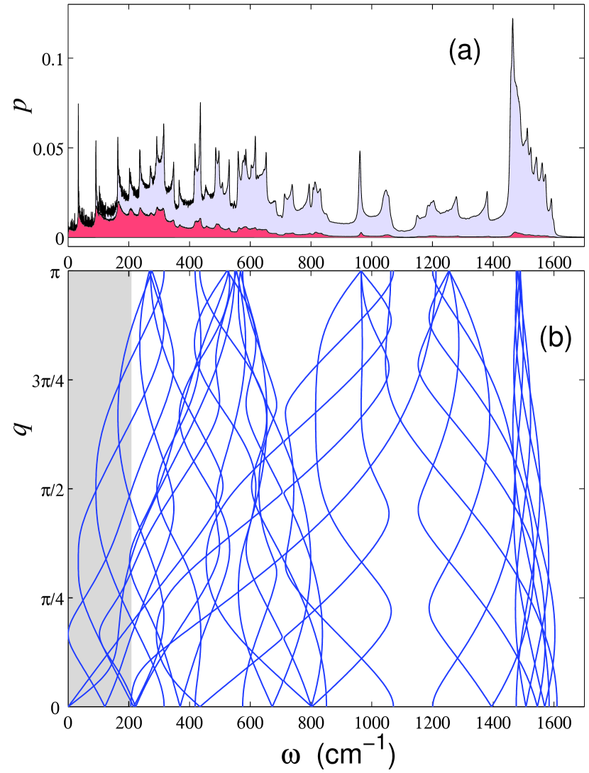
Figure 4: (a) Spectral density of thermal oscillations of armchair $(6,6)$ carbon nanotube for $T=300$ K (red field corresponds to system equations with color noise) and (b) sixty dispersion curves of the phonon modes. Gray color marks the frequency region $\omega<k_{B}T/\hbar$.

The computation of the eigenvalues (37) yields not only all the dispersion curves $\omega(q)$ but also the spectral density $p(\omega)$, normalized according to $\int_{0}^{\infty}p(\omega)d\omega=1$.

A simple method for obtaining the temperature dependence of the spectral density consists in making a simulation of the thermal vibrations of the carbon nanotube. To this aim, the system is first driven to thermal equilibrium using the usual Langevin equations with white noise

$$M\ddot{\bf x}_{n,l}={\bf F}_{n,l}-\Gamma M\dot{\bf x}_{n,l}+\Xi_{n,l},$$ (38)

with the dissipation coefficient $\Gamma=1/t_{r}$, $t_{r}$ - the relaxation time of atoms (it is reasonable to take $t_{r}=0.1$ps) and $\Xi_{n,l}=(\xi_{n,l,1},...,\xi_{n,l,6})$ - the six dimensional vector corresponding to the normally distributed random noises, describing the interaction of the particles located in the cell $(n,l)$ with the thermal bath. The characteristic correlation functions of these noises can be written as

$$\langle\xi_{n,k,i}(t_{1})\xi_{m,l,j}(t_{2})\rangle=2Mk_{B}T\delta_{nm}\delta_{kl}\delta_{ij}\delta(t_{1}-t_{2}),$$ (39)

where $k_{B}$ is the Boltzmann constant and $T$ - the temperature of the thermostat. After having set the initial coordinates (31) and velocities to zero, the numerical integration of the system of Langevin equations was performed over $t=20\hskip 1.42262ptt_{r}$. We then decoupled the thermalized system from the bath and calculated the spectral density $p(\omega)$ of the kinetic energy distribution of the atoms by following the real time dynamics of the isolated system. In order to increase the accuracy of the result, the spectral density was obtained from 100 independent thermalization processes and averaged over the atoms of the system.

The spectral density profile obtained at $T=300$ K is shown in Fig. 4 (a). We notice that at this temperature, the density profile is in good agreement with the shape of the dispersion curves, which can be seen as a weak manifestation of non-linearity effects. If one assumes that the proper vibrational modes of the carbon nanotube remain linear, then the specific heat of the nanotube can be deduced from the integral

$$c(T)=\int_{0}^{+\infty}c_{q}(\omega)p(\omega)d\omega,$$ (40)

$$c_{q}(\omega)=\left(\frac{\hbar\omega}{k_{B}T}\right)^{2}\frac{\exp(\hbar\omega/k_{B}T)}{[\exp(\hbar\omega/k_{B}T)-1]^{2}}$$

where $c_{q}(\omega)$ is the dimensionless thermal capacity of phonons with angular frequency $\omega$. This method to compute the heat capacity of carbon nanotubes was first used in Ref. sh1 ; sh2 .

This approach is remarkably practical since the specific heat of the system follows from the simple knowledge of the spectral density $p(\omega)$ of thermal vibrations . On the other hand, the spectral density can be deduced from the shape of the spectral curves, that is, by considering the later as the frequency spectrum of the harmonic modes in the nanotube. The heat capacity $c(T)$ of the carbon nanotube with index (6,6), (12,12) and (10,0) obtained in this way is shown in Fig. 5. It is clearly seen in this figure that the specific heat is practically insensitive to the index of the nanotube. Furthermore, the temperature dependence of the specific heat is linear in the regime $0<T<400$ K. This temperature behaviour of the specific heat is in concordance with previous theoretical works sh1 ; sh2 and confirms the experimental measures of the specific heat of titanium dioxide nanotubes sh3 .

We can equally obtain the spectral density that appears in Eq. (40) directly from dynamical simulations, i.e. by following thermal vibrations of atoms in the carbon nanotube at finite temperature $T>0$. As it can be checked in Fig. 5, numerical simulations show that these two approaches yield almost the same result (the spectral density has a weak temperature dependence).

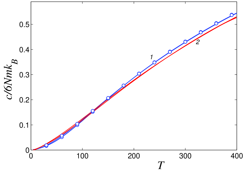
Figure 5: Temperature dependence of specific heat $c$ of carbon nanotube (6,6), (12,12) and (10,0). Blue line (curve 1) corresponds to the result obtained with the use of the frequency density of linear phonon waves while markers was obtained from the frequency density of thermal vibrations. Red line (curve 2) corresponds to the result obtained from the numerical integration of Langevin equations with color noise.

Let us notice that the numerical integration of the Langevin equations with white noise (38) that allows to obtain the dimensionless specific heat of the nanotube $(m,0)$ from the equation $c(T)=(d\langle H\rangle/dT)/(6Nmk_{B})$, where $Nh$ is the length of the nanotube, shows that the heat capacity is practically independent of the temperature, that is, $c=1$ over $0<T<400$ K (this results from the well-known equipartition theorem of classical statistical mechanics, which states that the mean energy of each degree of freedom is equal to $k_{B}T$). But the situation drastically changes, if one replaces the white noise of the Langevin equation with a time-correlated color noise whose temperature dependence is given by the formula (11). In this case, thermal vibrations of the nanotube are described by the system of Langevin equations

$$M\ddot{\bf x}_{n,l} = {\bf F}_{n,l}-\Gamma M\dot{\bf x}_{n,l}+\Xi_{n,l},$$ (41)

$$\dot{\Xi}_{n,l} = (\Theta_{n,l}-\Xi_{n,l})/t_{c},$$ (42)

where $\Theta_{n,l}=(\eta_{n,l,1},...,\eta_{n,l,6})$ - the six dimensional vector corresponding to the normally distributed random noise and normalized according to (39), the relaxation time $t_{r}=1$ ps and the correlation time of random noises, $t_{c}=\hbar\sqrt{e-2}/k_{B}T$.

The numerical integration of the equations of motion (41) and (42) first yields the mean energy of the nanotube $E=\langle H\rangle$ versus temperature $T$. Then the specific heat is deduced from the relation $c(T)=dE/dT$. The result is illustrated in Fig. 5. First of all, it is clearly seen that the specific heat of nanotubes (6,6), (12,12) and (10,0) have practically the same temperature behaviour, that is, it tends to zero for $T\rightarrow 0$ and it rises regularly with the increase of the temperature. Furthermore, the specific heat calculated with color noise coincides very well with the one obtained from Eq. (40) via computation of the spectral density.

We show in Fig. 4-(a) the shape of the spectral density of thermal vibrations of the carbon nanotube, obtained with color noise. We can note that only low frequency vibrations characterized by $\omega<k_{B}T/\hbar$ are totally thermalized while the thermalization of high frequency modes is partial. Moreover, the degree of thermalization decreases with increasing temperature.

By considering the concrete example of carbon nanotubes, we have shown that the use of the Langevin equations with color noise (41) and (42) allows to realize the quantum effect of partial thermalization of high frequency modes and yields the correct temperature behaviour of the specific heat for complex molecular systems. The proposed method becomes very useful especially for molecular systems with complex configurational dynamics, for example in the case of macromolecules which possess globular structure, or simply when one deals with a highly non-linear dynamics and it becomes meaningless to consider the existence of a spectral density of small-amplitude linear vibrations.

Let us mention a further application of the generalized Langevin approach. The formalism that we have presented consists in coupling to each particle a color noise of the same amplitude, which drives the systems to thermal equilibrium. If one instead couples the noise to chosen particles of the system or applies a noise of different amplitude to each particle, then the dynamics will be a non-equilibrium process. In this case, the use of the color noise may lead to new effects such as ratchet dynamics (see for ex. cl1 ; cl2 ), which can be obtained neither within the usual Langevin approach with white noise nor with a quantum description of the dynamics.

V Conclusions

We proposed a new method for computing the temperature dependence of the heat capacity in complex molecular systems. The proposed scheme is based on the use of the Langevin equation with low frequency color noise. We showed that the thermal behaviour of the correlation time of random forces, which is the key characteristic of the partial thermalization effect, can be described by a linear function of the inverse bath temperature, that is $t_{c}=\hbar\sqrt{e-2}/k_{B}T$. We next illustrated non-linearity effects by considering two simple Hamiltonian models and we explicitly showed that the generalized Langevin approach can be used in the presence of anharmonicities in the Hamiltonian. Finally, by applying the proposed procedure to carbon nanotubes, we showed that the consideration of the color noise in the Langevin equation allows to accurately reproduce the temperature evolution of the specific heat in many-body systems.

It is well-known that for complex systems having strong non-linearity effects in the quantum regime ($T<T_{E}$), there exists a temperature gap unreachable by existing approximative approaches such as the self-consistent phonon theory or the spectral density equations (40), while the drawback of quantum Monte-Carlo methods is the large numerical cost in the case of many particle models. The proposed method may be very useful to fill this gap, especially if one wishes to investigate the thermodynamics of realistic molecular systems with complex configurational dynamics, for example in the case of macromolecules which possess globular structures with a highly non-linear dynamics.

Appendix A The specific heat of the oscillator systems from Kleinert‘s variational Path Integral approach

We will give in this appendix the heat capacities of the simple non-linear oscillator systems (14) and (21), obtained from the first order variational path integral method. Since this approach has already been intensively discussed Kleinert ; Tognetti and applied to several many body problems TognettiII ; Liu ; Bao , we will omit the technical details of the procedure and only report the analytical form of the effective potential for each Hamiltonian.

The effective potential obtained by Feynman and Kleinert Kleinert for the quartic quantum oscillator (14) can be written as

$$W(x) = \frac{\beta}{4}x^{4}+\frac{1}{2}(1+3\beta a^{2})x^{2}+\frac{3\beta}{4}a^{4}$$ (43)

$$+ \frac{1-\Omega^{2}}{2}a^{2}+T\ln\left[\frac{2T}{\Omega}\sinh\left(\frac{\Omega}{2T}\right)\right],$$

where the smearing parameter $a$ and the frequency $\Omega$ are deduced from the following self-consistent equations :

$$a^{2} = \frac{1}{2\Omega}\coth\left(\frac{\Omega}{2T}\right)-\frac{T}{\Omega^{2}},$$

$$\Omega^{2} = 1+3\beta(a^{2}+x^{2}).$$ (44)

These equations are solved in ref. Kleinert by a numerical iteration scheme at each $x$ and $T$. Although this numerical procedure becomes very complicated when one deals with many body systems, it is shown in ref. Tognetti that the parameters $a$, $\Omega$ and the centroid potential $W(x)$ can be obtained for a one dimensional oscillator chain by Taylor expanding the equations (A) with respect to the non-linearity parameter $\beta$ at the order $0(\beta)$, then substituting the expansions in Eq. (43) and keeping only the terms of the same linear order, which finally yields the centroid potential in a fully analytical form. In the case of the quartic one-body potential (14), this procedure yields

$$W(x)=\frac{\beta}{4}x^{4}+f_{1}(T)x^{2}+f_{2}(T),$$ (45)

where we have defined

$$f_{1}(T) = \frac{1}{2}-\frac{3\beta}{2}T+\frac{3\beta}{4}\coth\left(\frac{1}{2T}\right)$$

$$f_{2}(T) = \frac{3\beta}{16}\left[2T-\coth\left(\frac{1}{2T}\right)\right]^{2}$$

$$+ T\ln\left[2T\sinh\left(\frac{1}{2T}\right)\right].$$

The partition function that follows from Eq. (45) and (20) can now be expressed in terms of the Bessel function of the second kind as

$$Z=\sqrt{\frac{f_{1}}{\beta}}\exp\left(\frac{f_{1}^{2}-2\beta f_{2}}{2\beta T}\right)\mathbf{K}_{\frac{1}{4}}\left(\frac{f_{1}^{2}}{2\beta T}\right)$$ (47)

and the specific heat is deduced from Eq. (16).

The effective potential of the two-body Hamiltonian (21) is computed in a similar way as for one dimensional oscillator chains Tognetti . The trial action that appears in Eq. (19) was chosen in the form

$$S_{0}=\int d\tau \left\{\frac{1}{2}\left(\dot{x}^{2}+\dot{y}^{2}\right)+\frac{\lambda_{x}}{2}(x-x_{0})^{2}\right.$$ (48)

$$+ \left.\frac{\lambda_{y}}{2}(y-y_{0})^{2}+g(x-x_{0})(y-y_{0})\right\}.$$

where $\lambda_{x}$, $\lambda_{y}$ and $g$ denote the trial parameters that minimize the Jensen-Peirels inequality (19). After going through the usual minimization procedure and expanding the smearing parameter $a$ and the centroid potential at the order $0(\beta)$, one obtains

$$a_{0}^{2}= - T\frac{\omega_{x}^{2}+\omega_{y}^{2}}{\omega_{x}^{2}\hskip 1.42262pt\omega_{y}^{2}}$$

$$+ \frac{1}{2\omega_{x}\hskip 1.42262pt\omega_{y}}\left\{\omega_{x}\coth\left(\frac{\omega_{y}}{2T}\right)+\omega_{y}\coth\left(\frac{\omega_{x}}{2T}\right)\right\},$$

$$W(x,y)= - T\ln\left\{\frac{\omega_{x}\omega_{y}}{4T^{2}}\frac{1}{\sinh(\omega_{x}/2T)\sinh(\omega_{y}/2T)}\right\}$$ (49)

$$+ \frac{\omega_{x}^{2}}{2}x^{2}+\frac{\omega_{y}^{2}}{2}y^{2}+\frac{3\beta}{4}a_{0}^{4}$$

$$+ \frac{\beta}{4}(x-y)^{4}+\frac{3\beta}{2}a_{0}^{2}(x-y)^{2}.$$

The integration in Eq. (20) can be carried out analytically by performing the coordinate transformation

$$u=\frac{x-y}{\sqrt{2}},\hskip 28.45274ptv=\frac{x+y}{\sqrt{2}}.$$ (50)

We finally obtain for the partition function

$$Z = \frac{\Omega\hskip 1.42262pt\omega_{x}\omega_{y}}{8\sqrt{\pi\beta T(\omega_{x}^{2}+\omega_{y}^{2})}}\frac{1}{\sinh(\omega_{x}/2T)\sinh(\omega_{y}/2T)}$$ (51)

$$\times \exp\left(-\frac{6\beta^{2}a_{0}^{4}+\Omega^{4}}{8\beta T}\right)\mathbf{K}_{\frac{1}{4}}\left(\frac{\Omega^{4}}{8\beta T}\right)$$

where we have defined

$$\Omega^{2}=\frac{\omega_{x}^{2}\hskip 1.42262pt\omega_{y}^{2}}{\omega_{x}^{2}+\omega_{y}^{2}}+3\beta a_{0}^{2}.$$ (52)

References

• (1) A. Einstein, Ann. Phys., 22, 180 (1907).
• (2) R. P. Feynman, H. Kleinert, Phys. Rev. A 34, 5080 (1986).
• (3) R. Giachetti, V. Tognetti, Phys. Rev. B 33, 7647 (1986).
• (4) D.W. Noid et al., Macromolecules 24, 4148 (1991).
• (5) B.G. Sumpter et al. Adv. Polym. Sci. 116, 27 (1994).
• (6) A.V. Savin and L.I. Manevitch, Phys. Rev. B 58, 11386 (1998); Phys. Rev. B 67, 144302 (2003).
• (7) R. Al-Jishi and G. Dresselhaus, Phys. Rev. B 26, 4514 (1982).
• (8) T. Aizawa, R. Souda, S. Otani, Y. Ishizawa, C. Oshima, Phys. Rev. B 42, 11469 (1990).
• (9) V.N. Popov, Phys. Rev. B 66, 153408 (2002).
• (10) J. X. Cao, X. H. Yan, Y. Xiao, Y. Tang, J. W. Ding, Phys. Rev. B 67, 045413 (2003).
• (11) C. Dames et al., Appl. Phys. Lett. 87, 031901 (2005).
• (12) P. Reimann, Phys. Rev. Lett. 86, 4992 (2001)
• (13) S. Denisov, S. Flach, A.A. Ovchinnikov, O. Yevtushenko, Y. Zolotaryuk, Phys. Rev. E 66, 041104 (2002)
• (14) R. Giachetti, V. Tognetti, R. Vaia, Phys. Rev. A 38, 1638 (1988).
• (15) S. Liu, G. K. Horton, E. R. Cowley, Phys. Rev. B 44, 11714 (1991).
• (16) J. D. Bao, Y. Z. Zhuo, X. Z. Wu, Phys. Rev. E 52, 5656 (1995).