INSTITUT NATIONAL DE RECHERCHE EN INFORMATIQUE ET EN AUTOMATIQUE

Computing a Finite Size Representation of the Set of Approximate Solutions of an MOP111Parts of this manuscript will be published in the Proceedings of the Genetic and Evolutionary Computation Conference (GECCO-2008).
Oliver Schütze1, Carlos A. Coello Coello1, Emilia Tantar2 and El-Ghazali Talbi1
3 CINVESTAV-IPN, Computer Science Department
e-mail: {schuetze,ccoello}@cs.cinvestav.mx
1 INRIA Futurs, LIFL, CNRS Bât M3, Cité Scientifique
e-mail: {emilia.tantar,talbi}@lifl.fr
N° 6492
April 2008

Computing a Finite Size Representation of the Set of Approximate Solutions of an MOP***Parts of this manuscript will be published in the Proceedings of the Genetic and Evolutionary Computation Conference (GECCO-2008).


Oliver Schütze1, Carlos A. Coello Coello1, Emilia Tantar2 and El-Ghazali Talbi1

3 CINVESTAV-IPN, Computer Science Department
e-mail: {schuetze,ccoello}@cs.cinvestav.mx

1 INRIA Futurs, LIFL, CNRS Bât M3, Cité Scientifique
e-mail: {emilia.tantar,talbi}@lifl.fr

Thèmes COM et COG et SYM et NUM et BIO — Systèmes communicants et Systèmes cognitifs et Systèmes symboliques et Systèmes numériques et Systèmes biologiques

Projets Apics et Opéra

Rapport de recherche n° 6492 — April 2008 — ?? pages

Abstract: Recently, a framework for the approximation of the entire set of ϵitalic-ϵ\epsilon-efficient solutions (denote by Eϵsubscript𝐸italic-ϵE_{\epsilon}) of a multi-objective optimization problem with stochastic search algorithms has been proposed. It was proven that such an algorithm produces – under mild assumptions on the process to generate new candidate solutions –a sequence of archives which converges to Eϵsubscript𝐸italic-ϵE_{\epsilon} in the limit and in the probabilistic sense. The result, though satisfactory for most discrete MOPs, is at least from the practical viewpoint not sufficient for continuous models: in this case, the set of approximate solutions typically forms an n𝑛n-dimensional object, where n𝑛n denotes the dimension of the parameter space, and thus, it may come to perfomance problems since in practise one has to cope with a finite archive.
Here we focus on obtaining finite and tight approximations of Eϵsubscript𝐸italic-ϵE_{\epsilon}, the latter measured by the Hausdorff distance. We propose and investigate a novel archiving strategy theoretically and empirically. For this, we analyze the convergence behavior of the algorithm, yielding bounds on the obtained approximation quality as well as on the cardinality of the resulting approximation, and present some numerical results.

Key-words: multi-objective optimization, convergence, ϵitalic-ϵ\epsilon-efficient solutions, approximate solutions, stochastic search algorithms.

Computing a Finite Size Representation of the Set of Approximate Solutions of an MOP

Résumé : Dans des travaux précédent, nous avons proposé un environnement (”framework”) pour l’approximation de l’intégralité de l’ensemble des solutions ϵitalic-ϵ\epsilon-efficaces (noté Eϵsubscript𝐸italic-ϵE_{\epsilon}) d’un problème d’optimisation multi-objectifs à l’aide d’une recherche stochastique. Il a été prouvé que suivant certaines hypothèses relatives au processus de génération de nouvelles solutions candidates, un tel algorithme produit une séquence d’archives qui converge asymptotiquement vers Eϵsubscript𝐸italic-ϵE_{\epsilon}, au sens probabiliste du terme. Le résultat, s’il est satisfaisant pour la plupart des MOP discrets, ne l’est pas d’un point de vue pratique pour les problèmes continus. Dans ce dernier cas, l’ensemble des solutions approximées forme un objet à n𝑛n dimentions, où n𝑛n est la dimension de l’espace des paramètres. Ceci peut amener à des problèmes de performances puisqu’en pratique la taille de l’archive est finie.

Dans le travail présenté, nous nous concentrons sur l’obtention d’approximations finies et précises de Eϵsubscript𝐸italic-ϵE_{\epsilon} qui est mesuré par la distance de Hausdorff. Nous proposons et nous étudions une nouvelle stratégie d’archivage des points de vue théorique et pratique. Pour ce faire, nous analysons le comportement asymptotique de l’algorithme, en fournissant les limites de qualité de l’approximation obtenue, aussi bien que la cardinalité de l’approximation et nous présentons également quelques résultats numériques.

Mots-clés : optimisation multi-objectif, convergence, solutions ϵitalic-ϵ\epsilon-efficaces, solutions approwimées, algorithmes de recherche stochastique.

1 Introduction

Since the notion of ϵitalic-ϵ\epsilon-efficiency for multi-objective optimization problems (MOPs) has been introduced more than two decades ago ([8]), this concept has been studied and used by many researchers, e.g. to allow (or tolerate) nearly optimal solutions ([8], [18]), to approximate the set of optimal solutions ([11]), or in order to discretize this set ([7], [14]). ϵitalic-ϵ\epsilon-efficient solutions or approximate solutions have also been used to tackle a variety of real world problems including portfolio selection problems ([19]), a location problem ([2]), or a minimal cost flow problem ([11]).
As an illustrative example where it could make sense from the practical point of view to consider in addition to the exact solutions also approximate ones we consider a plane truss design problem, where the volume of the truss as well as the displacement of the joint to a given position have to be minimized (see also Section 6.2). Since the designs of this problem – as basically in all other engineering problems – have to obey certain physical contraints such as in this case the weight and stability of the structural element, the objective values of all feasible solutions are located within a relatively tight and a priori appreciable range. Hence, the maximal tolerable loss of a design compared to an ‘optimal’ one with respect to the objective values can easily be determined quantitatively and qualitatively by the decision maker (DM) before the optimization process. The resulting set of exact and approximate (but physically relevant) solutions obtained by the optimization algorithm111Here we assume an idealized algorithm, since in practise every solution is an approximate one. leads in general to a larger variety of possibilities to the DM than ‘just’ the set of exact solutions: this is due to the fact that solutions which are ‘near’ in objective space can differ significantly in design space (e.g., when the model contains symmetries, or see Section 6.3 for another example).
The computation of such approximate solutions has been addressed in several studies. In most of them, scalarization methods have been empoyed (e.g., [18], [2], [4]). By their nature, such algorithms can deliver only single solutions by one single execution. The only work so far which deals with the approximation of the entire set of approximate solutions (denote by Eϵsubscript𝐸italic-ϵE_{\epsilon}) is [13], where an archiving strategy for stochastic search algorithms is proposed for this task. Such a sequence of archives obtained by this algorithm provably converges – under mild assumptions on the process to generate new candidate solutions – to Eϵsubscript𝐸italic-ϵE_{\epsilon} in the limit and in the probabilistic sense. This result, though satisfactory for most discrete MOPs, is at least from the practical viewpoint not sufficient for continuous models (i.e., continous objectives defined on a continuous domain): in this case, the set of approximate solutions typically forms an n𝑛n-dimensional object, where n𝑛n denotes the dimension of the parameter space (see below). Thus, it may come to performance problems since it can easily happen that a given threshold on the magnitude of the archives is exceeded before a ‘sufficient’ approximation of the set of interest in terms of diversity and/or convergence is obtained. An analogue statement holds for the approximation of the Pareto front, which is ‘only’ (k1)𝑘1(k-1)-dimensional for MOPs with k𝑘k objectives, and suitable discretizations have been subject of research since several years (e.g., [7], [6], [14]).
The scope of this paper is to develop a framework for finite size representations of the set Eϵsubscript𝐸italic-ϵE_{\epsilon} with stochastic search algorithms such as evolutionary multi-objective (EMO) algorithms. This will call for the design of a novel archiving strategy to store the ‘required’ solutions found by the stochastic search process. We will further analyze the convergence behavior of this method, yielding bounds on the approximation quality as well as on the cardinality of the resulting approximations. Finally, we will demonstrate the practicability of the novel approach by several examples.

The remainder of this paper is organized as follows: in Section 2, we state the required background including the set of interest PQ,ϵsubscript𝑃𝑄italic-ϵP_{Q,\epsilon}. In Section 3, we propose a novel archiving strategy for the approximation of PQ,ϵsubscript𝑃𝑄italic-ϵP_{Q,\epsilon} and state a convergence result, and give further on an upper bound on the resulting archive sizes in Section 4. In Section 5, we present some numerical results, and make finally some conclusions in Section 6.

2 Background

In the following we consider continuous multi-objective optimization problems

minxQ{F(x)},subscript𝑥𝑄𝐹𝑥\min_{x\in Q}\{F(x)\}, (MOP)

where Qn𝑄superscript𝑛Q\subset\mathbbm{R}^{n} and F𝐹F is defined as the vector of the objective functions F:Qk,F(x)=(f1(x),,fk(x)),:𝐹formulae-sequence𝑄superscript𝑘𝐹𝑥subscript𝑓1𝑥subscript𝑓𝑘𝑥F:Q\to\mathbbm{R}^{k},\quad F(x)=(f_{1}(x),\ldots,f_{k}(x)), and where each fi:Q:subscript𝑓𝑖𝑄f_{i}:Q\to\mathbbm{R} is continuously differentiable. Later we will restrict the search to a compact set Q𝑄Q, the reader may think of an n𝑛n-dimensional box.

Definition 2.1
  1. (a)

    Let v,wQ𝑣𝑤𝑄v,w\in Q. Then the vector v𝑣v is less than w𝑤w (v<pwsubscript𝑝𝑣𝑤v<_{p}w), if vi<wisubscript𝑣𝑖subscript𝑤𝑖v_{i}<w_{i} for all i{1,,k}𝑖1𝑘i\in\{1,\ldots,k\}. The relation psubscript𝑝\leq_{p} is defined analogously.

  2. (b)

    yn𝑦superscript𝑛y\in\mathbbm{R}^{n} is dominated by a point xQ𝑥𝑄x\in Q (xyprecedes𝑥𝑦x\prec y) with respect to (MOP) if F(x)pF(y)subscript𝑝𝐹𝑥𝐹𝑦F(x)\leq_{p}F(y) and F(x)F(y)𝐹𝑥𝐹𝑦F(x)\neq F(y), else y𝑦y is called nondominated by x𝑥x.

  3. (c)

    xQ𝑥𝑄x\in Q is called a Pareto point if there is no yQ𝑦𝑄y\in Q which dominates x𝑥x.

The set of all Pareto optimal solutions is called the Pareto set (denote by PQsubscript𝑃𝑄P_{Q}). This set typically – i.e., under mild regularity assumptions – forms a (k1)𝑘1(k-1)-dimensional object. The image of the Pareto set is called the Pareto front.
We now define another notion of dominance, which is the basis of the approximation concept used in this study.

Definition 2.2

Let ϵ=(ϵ1,,ϵk)+kitalic-ϵsubscriptitalic-ϵ1subscriptitalic-ϵ𝑘subscriptsuperscript𝑘\epsilon=(\epsilon_{1},\ldots,\epsilon_{k})\in\mathbbm{R}^{k}_{+} and x,yQ𝑥𝑦𝑄x,y\in Q.

  1. (a)

    x𝑥x is said to ϵitalic-ϵ\epsilon-dominate y𝑦y (xϵysubscriptprecedesitalic-ϵ𝑥𝑦x\prec_{\epsilon}y) with respect to (MOP) if F(x)ϵpF(y)subscript𝑝𝐹𝑥italic-ϵ𝐹𝑦F(x)-\epsilon\leq_{p}F(y) and F(x)ϵF(y)𝐹𝑥italic-ϵ𝐹𝑦F(x)-\epsilon\neq F(y).

  2. (b)

    x𝑥x is said to ϵitalic-ϵ-\epsilon-dominate y𝑦y (xϵysubscriptprecedesitalic-ϵ𝑥𝑦x\prec_{-\epsilon}y) with respect to (MOP) if F(x)+ϵpF(y)subscript𝑝𝐹𝑥italic-ϵ𝐹𝑦F(x)+\epsilon\leq_{p}F(y) and F(x)+ϵF(y)𝐹𝑥italic-ϵ𝐹𝑦F(x)+\epsilon\neq F(y).

The notion of ϵitalic-ϵ-\epsilon-dominance is of course analogous to the ‘classical’ ϵitalic-ϵ\epsilon-dominance relation but with a value ϵ~k~italic-ϵsubscriptsuperscript𝑘\tilde{\epsilon}\in\mathbbm{R}^{k}_{-}. However, we highlight it here since it will be used frequently in this work. While the ϵitalic-ϵ\epsilon-dominance is a weaker concept of dominance, ϵitalic-ϵ-\epsilon-dominance is a stronger one.
We now define the set which we want to approximate in the sequel.

Definition 2.3

Denote by PQ,ϵsubscript𝑃𝑄italic-ϵP_{Q,\epsilon} the set of points in Qn𝑄superscript𝑛Q\subset\mathbbm{R}^{n} which are not ϵitalic-ϵ-\epsilon-dominated by any other point in Q𝑄Q, i.e.

PQ,ϵ:={xQ|yQ:yϵx}.assignsubscript𝑃𝑄italic-ϵconditional-set𝑥𝑄:not-exists𝑦𝑄subscriptprecedesitalic-ϵ𝑦𝑥P_{Q,\epsilon}:=\{x\in Q|\not\exists y\in Q:y\prec_{-\epsilon}x\}. (1)

To see that PQ,ϵsubscript𝑃𝑄italic-ϵP_{Q,\epsilon} typically forms an n𝑛n-dimensional set let x0PQsubscript𝑥0subscript𝑃𝑄x_{0}\in P_{Q} (such a point, for instance, always exists if Q𝑄Q is compact). That is, there exists no yQ𝑦𝑄y\in Q such that yx0precedes𝑦subscript𝑥0y\prec x_{0}. Since F𝐹F is continuous and ϵ+kitalic-ϵsubscriptsuperscript𝑘\epsilon\in\mathbbm{R}^{k}_{+} there exists a neigborhood U𝑈U of x0subscript𝑥0x_{0} such that

yQ:yϵuuUQ,:not-exists𝑦𝑄formulae-sequencesubscriptprecedesitalic-ϵ𝑦𝑢for-all𝑢𝑈𝑄\not\exists y\in Q:\;y\prec_{-\epsilon}u\quad\forall u\in U\cap Q, (2)

and thus, UQPQ,ϵ𝑈𝑄subscript𝑃𝑄italic-ϵU\cap Q\subset P_{Q,\epsilon}, and we are done since U𝑈U is n𝑛n-dimensional.
The following result and notions are used for the upcoming proof of convergence.

Theorem 2.4 ([12])

Let (MOP) be given and q:nn:𝑞superscript𝑛superscript𝑛q:\mathbbm{R}^{n}\to\mathbbm{R}^{n} be defined by q(x)=i=1kα^ifi(x)𝑞𝑥superscriptsubscript𝑖1𝑘subscript^𝛼𝑖subscript𝑓𝑖𝑥q(x)=\sum_{i=1}^{k}\hat{\alpha}_{i}\nabla f_{i}(x), where α^^𝛼\hat{\alpha} is a solution of

minαk{i=1kαifi(x)22;αi0,i=1,,k,i=1kαi=1}.subscript𝛼superscript𝑘superscriptsubscriptnormsuperscriptsubscript𝑖1𝑘subscript𝛼𝑖subscript𝑓𝑖𝑥22subscript𝛼𝑖0𝑖1𝑘superscriptsubscript𝑖1𝑘subscript𝛼𝑖1\min_{\alpha\in\mathbbm{R}^{k}}\left\{\left\|\sum_{i=1}^{k}\alpha_{i}\nabla f_{i}(x)\right\|_{2}^{2};\alpha_{i}\geq 0,i=1,\ldots,k,\sum_{i=1}^{k}\alpha_{i}=1\right\}.

Then either q(x)=0𝑞𝑥0q(x)=0 or q(x)𝑞𝑥-q(x) is a descent direction for all objective functions f1,,fksubscript𝑓1subscript𝑓𝑘f_{1},\ldots,f_{k} in x𝑥x. Hence, each x𝑥x with q(x)=0𝑞𝑥0q(x)=0 fulfills the first-order necessary condition for Pareto optimality.

Definition 2.5

Let un𝑢superscript𝑛u\in\mathbbm{R}^{n} and A,Bn𝐴𝐵superscript𝑛A,B\subset\mathbbm{R}^{n}. The semi-distance dist(,)dist\mbox{dist}(\cdot,\cdot) and the Hausdorff distance dH(,)subscript𝑑𝐻d_{H}(\cdot,\cdot) are defined as follows:

  • (a)

    dist(u,A):=infvAuvassigndist𝑢𝐴subscriptinfimum𝑣𝐴norm𝑢𝑣\mbox{dist}(u,A):=\inf\limits_{v\in A}\|u-v\|

  • (b)

    dist(B,A):=supuBdist(u,A)assigndist𝐵𝐴subscriptsupremum𝑢𝐵dist𝑢𝐴\mbox{dist}(B,A):=\sup\limits_{u\in B}\,\mbox{dist}(u,A)

  • (c)

    dH(A,B):=max{dist(A,B),dist(B,A)}assignsubscript𝑑𝐻𝐴𝐵dist𝐴𝐵dist𝐵𝐴d_{H}(A,B):=\max\left\{\mbox{dist}(A,B),\mbox{dist}(B,A)\right\}

Denote by A¯¯𝐴\overline{A} the closure of a set An𝐴superscript𝑛A\in\mathbbm{R}^{n}, by A𝐴\overset{\circ}{A} its interior, and by A=A¯\A𝐴\¯𝐴𝐴\partial A=\overline{A}\backslash\overset{\circ}{A} the boundary of A𝐴A.

Definition 2.6
  1. (a)

    A point xQ𝑥𝑄x\in Q is called a weak Pareto point if there exists no point yQ𝑦𝑄y\in Q such that F(y)<pF(x)subscript𝑝𝐹𝑦𝐹𝑥F(y)<_{p}F(x).

  2. (b)

    A point xQ𝑥𝑄x\in Q is called ϵitalic-ϵ-\epsilon weak Pareto point if there exists no point yQ𝑦𝑄y\in Q such that F(y)+ϵ<pF(x)subscript𝑝𝐹𝑦italic-ϵ𝐹𝑥F(y)+\epsilon<_{p}F(x).

Algorithm 1 gives a framework of a generic stochastic multi-objective optimization algorithm, which will be considered in this work. Here, Qn𝑄superscript𝑛Q\subset\mathbbm{R}^{n} denotes the domain of the MOP, Pjsubscript𝑃𝑗P_{j} the candidate set (or population) of the generation process at iteration step j𝑗j, and Ajsubscript𝐴𝑗A_{j} the corresponding archive.

Algorithm 1 Generic Stochastic Search Algorithm
1:P0Qsubscript𝑃0𝑄P_{0}\subset Q drawn at random
2:A0=ArchiveUpdate(P0,)subscript𝐴0𝐴𝑟𝑐𝑖𝑣𝑒𝑈𝑝𝑑𝑎𝑡𝑒subscript𝑃0A_{0}=ArchiveUpdate(P_{0},\emptyset)
3:for j=0,1,2,𝑗012j=0,1,2,\ldots do
4:     Pj+1=Generate(Pj)subscript𝑃𝑗1𝐺𝑒𝑛𝑒𝑟𝑎𝑡𝑒subscript𝑃𝑗P_{j+1}=Generate(P_{j})
5:     Aj+1=ArchiveUpdate(Pj+1,Aj)subscript𝐴𝑗1𝐴𝑟𝑐𝑖𝑣𝑒𝑈𝑝𝑑𝑎𝑡𝑒subscript𝑃𝑗1subscript𝐴𝑗A_{j+1}=ArchiveUpdate(P_{j+1},A_{j})
6:end for

3 The Algorithm

Here we present and analyze a novel archiving strategy which aims for a finite size representation of PQ,ϵsubscript𝑃𝑄italic-ϵP_{Q,\epsilon}.
The algorithm which we propose here, ArchiveUpdatePQ,ϵ𝐴𝑟𝑐𝑖𝑣𝑒𝑈𝑝𝑑𝑎𝑡𝑒subscript𝑃𝑄italic-ϵArchiveUpdateP_{Q,\epsilon}, is given in Algorithm 2. Denote by 1Δ:=(Δ,,Δ)+kassign1ΔΔΔsuperscriptsubscript𝑘1\Delta:=(\Delta,\ldots,\Delta)\in\mathbbm{R}_{+}^{k}, where Δ+Δsubscript\Delta\in\mathbbm{R}_{+} can be viewed as the discretization parameter of the algorithm.

Algorithm 2 A:=ArchiveUpdatePQ,ϵ(P,A0,Δ)assign𝐴𝐴𝑟𝑐𝑖𝑣𝑒𝑈𝑝𝑑𝑎𝑡𝑒subscript𝑃𝑄italic-ϵ𝑃subscript𝐴0ΔA:=ArchiveUpdateP_{Q,\epsilon}\;(P,A_{0},\Delta)
1:population P𝑃P, archive A0subscript𝐴0A_{0}, Δ+Δsubscript\Delta\in\mathbbm{R}_{+}, Δ(0,Δ)superscriptΔ0Δ\Delta^{*}\in(0,\Delta)
2:updated archive A𝐴A
3:A:=A0assign𝐴subscript𝐴0A:=A_{0}
4:for all pP𝑝𝑃p\in P do
5:     if a1A:aϵpanda2A:d(F(a),F(p))Δ:not-existssubscript𝑎1𝐴subscriptprecedesitalic-ϵ𝑎𝑝andnot-existssubscript𝑎2𝐴:subscript𝑑𝐹𝑎𝐹𝑝superscriptΔ\not\exists a_{1}\in A:\;a\prec_{-\epsilon}p\;\mbox{and}\;\not\exists a_{2}\in A:\;d_{\infty}(F(a),F(p))\leq\Delta^{*} then
6:         A:=A{p}assign𝐴𝐴𝑝A:=A\cup\{p\}
7:         for all aA𝑎𝐴a\in A do
8:              if p(ϵ+1Δ)asubscriptprecedesitalic-ϵ1Δ𝑝𝑎p\prec_{-(\epsilon+1\Delta)}a then
9:                  A:=A\{a}assign𝐴\𝐴𝑎A:=A\backslash\{a\}
10:              end if
11:         end for
12:     end if
13:end for
Lemma 3.1

Let A0,Pnsubscript𝐴0𝑃superscript𝑛A_{0},P\subset\mathbbm{R}^{n} be finite sets, ϵ+kitalic-ϵsuperscriptsubscript𝑘\epsilon\in\mathbbm{R}_{+}^{k}, Δ+Δsubscript\Delta\in\mathbbm{R}_{+}, and
A:=ArchiveUpdateEps1(P,A0)assign𝐴italic-ArchiveUpdateEps1𝑃subscript𝐴0A:=\mathit{ArchiveUpdateEps1}\;(P,A_{0}). Then the following holds:

xPA0:aA:a1Δx.\forall x\in P\cup A_{0}:\quad\exists a\in A:a\prec_{1\Delta}x.
Proof.

This follows immediately by the construction of the algorithm. ∎

Theorem 3.2

Let an MOP F:nk:𝐹superscript𝑛superscript𝑘F:\mathbbm{R}^{n}\to\mathbbm{R}^{k} be given, where F𝐹F is continuous, let Qn𝑄superscript𝑛Q\subset\mathbbm{R}^{n} be a compact set and ϵ+kitalic-ϵsubscriptsuperscript𝑘\epsilon\in\mathbbm{R}^{k}_{+}, Δ,Δ+ΔsuperscriptΔsubscript\Delta,\Delta^{*}\in\mathbbm{R}_{+} with Δ<ΔsuperscriptΔΔ\Delta^{*}<\Delta. For the generation process we assume

xQandδ>0:P(l:PlBδ(x)Q)=1\begin{split}\forall x\in Q\;\mbox{and}\;\forall\delta>0:\quad P\left(\exists l\in\mathbbm{N}\;:\;P_{l}\cap B_{\delta}(x)\cap Q\neq\emptyset\right)=1\end{split} (3)

and for the MOP

  • (A1)

    Let there be no weak Pareto point in Q\PQ\𝑄subscript𝑃𝑄Q\backslash P_{Q}.

  • (A2)

    Let there be no ϵitalic-ϵ-\epsilon weak Pareto point in Q\PQ,ϵ¯\𝑄¯subscript𝑃𝑄italic-ϵQ\backslash\overline{P_{Q,\epsilon}},

  • (A3)

    Define :={xQ|yPQ:F(y)+ϵ=F(x)}assignconditional-set𝑥𝑄:𝑦subscript𝑃𝑄𝐹𝑦italic-ϵ𝐹𝑥{\cal B}:=\{x\in Q|\exists y\in P_{Q}:F(y)+\epsilon=F(x)\}. Let Q𝑄{\cal B}\subset\overset{\circ}{Q} and q(x)0𝑞𝑥0q(x)\neq 0 for all x𝑥x\in{\cal B}, where q𝑞q is as defined in Theorem 2.4.

Then, an application of Algorithm 1, where
AchiveUpdatePQ,ϵ(P,A,Δ)𝐴𝑐𝑖𝑣𝑒𝑈𝑝𝑑𝑎𝑡𝑒subscript𝑃𝑄italic-ϵ𝑃𝐴ΔAchiveUpdateP_{Q,\epsilon}(P,A,\Delta) is used to update the archive, leads to a sequence of archives Al,lsubscript𝐴𝑙𝑙A_{l},l\in\mathbbm{N}, where the following holds:

  • (a)

    For all l𝑙l\in\mathbbm{N} it holds

    F(a1)F(a2)Δsubscriptnorm𝐹subscript𝑎1𝐹subscript𝑎2superscriptΔ\|F(a_{1})-F(a_{2})\|_{\infty}\geq\Delta^{*} (4)
  • (b)

    There exists with probability one an l0subscript𝑙0l_{0}\in\mathbbm{N} such that for all ll0𝑙subscript𝑙0l\geq l_{0}:

    • (b1)

      dist(F(PQ,ϵ),F(Al))<Δ𝑑𝑖𝑠𝑡𝐹subscript𝑃𝑄italic-ϵ𝐹subscript𝐴𝑙Δdist(F(P_{Q,\epsilon}),F(A_{l}))<\Delta

    • (b2)

      dist(F(Al),F(PQ,ϵ))dist(F(PQ,ϵ+2Δ),F(PQ,ϵ))𝑑𝑖𝑠𝑡𝐹subscript𝐴𝑙𝐹subscript𝑃𝑄italic-ϵ𝑑𝑖𝑠𝑡𝐹subscript𝑃𝑄italic-ϵ2Δ𝐹subscript𝑃𝑄italic-ϵdist(F(A_{l}),F(P_{Q,\epsilon}))\leq dist(F(P_{Q,\epsilon+2\Delta}),F(P_{Q,\epsilon}))

    • (b3)

      dH(F(PQ,ϵ),F(Al))Dsubscript𝑑𝐻𝐹subscript𝑃𝑄italic-ϵ𝐹subscript𝐴𝑙𝐷d_{H}(F(P_{Q,\epsilon}),F(A_{l}))\leq D, where
      D=max(Δ,dist(F(PQ,ϵ+2Δ),F(PQ,ϵ))D=max(\Delta,dist(F(P_{Q,\epsilon+2\Delta}),F(P_{Q,\epsilon}))

Proof.

Before we state the proof we have to make some remarks: a point p𝑝p is discarded from an existing archive A𝐴A in two cases (see line 3 of Algorithm 2):

(D1)a1A:a1ϵp,or(D2)a2A:F(a2)F(p)Δ.\begin{split}(D1)&\quad\exists a_{1}\in A:\;a_{1}\prec_{-\epsilon}p,\quad\mbox{or}\\ (D2)&\quad\exists a_{2}\in A:\;\|F(a_{2})-F(p)\|_{\infty}\leq\Delta^{*}.\end{split} (5)

Further, we define by

Bδ(x):={yk:xy<δ}assignsubscriptsuperscript𝐵𝛿𝑥conditional-set𝑦superscript𝑘subscriptnorm𝑥𝑦𝛿B^{\infty}_{\delta}(x):=\{y\in\mathbbm{R}^{k}\,:\,\|x-y\|_{\infty}<\delta\}

a k𝑘k-dimensional open box around xk𝑥superscript𝑘x\in\mathbbm{R}^{k}. Now we are in the position to state the proof.

Claim (a): follows immediately by construction of the algorithm and by an inductive argument.
Claim (b1): By (a) it follows that for an element a𝑎a from a given archive A𝐴A it holds

F(a~)BΔ(F(a)),a~A\{a},formulae-sequence𝐹~𝑎subscriptsuperscript𝐵superscriptΔ𝐹𝑎for-all~𝑎\𝐴𝑎F(\tilde{a})\not\in B^{\infty}_{\Delta^{*}}(F(a)),\quad\forall\tilde{a}\in A\backslash\{a\}, (6)

Since further Q𝑄Q is compact and F𝐹F is continuous it follows that F(Q)𝐹𝑄F(Q) is bounded, and thus, there exits an upper bound for the number of entries in the archive for a given MOP, denote by n0=n0(Δ,F(Q))subscript𝑛0subscript𝑛0superscriptΔ𝐹𝑄n_{0}=n_{0}(\Delta^{*},F(Q)) (see also Section 4).
Since PQ,ϵ¯¯subscript𝑃𝑄italic-ϵ\overline{P_{Q,\epsilon}} is compact and
dist(F(PQ,ϵ),F(Al))=dist(F(PQ,ϵ¯),F(Al))𝑑𝑖𝑠𝑡𝐹subscript𝑃𝑄italic-ϵ𝐹subscript𝐴𝑙𝑑𝑖𝑠𝑡𝐹¯subscript𝑃𝑄italic-ϵ𝐹subscript𝐴𝑙dist(F(P_{Q,\epsilon}),F(A_{l}))=dist(F(\bar{P_{Q,\epsilon}}),F(A_{l})), and since Al,lsubscript𝐴𝑙𝑙A_{l},l\in\mathbbm{N}, is finite it follows that

dist(F(PQ,ϵ),F(Al))=maxpPQ,ϵminaAlF(p)F(a)𝑑𝑖𝑠𝑡𝐹subscript𝑃𝑄italic-ϵ𝐹subscript𝐴𝑙subscript𝑝subscript𝑃𝑄italic-ϵsubscript𝑎subscript𝐴𝑙subscriptnorm𝐹𝑝𝐹𝑎dist(F(P_{Q,\epsilon}),F(A_{l}))=\max\limits_{p\in P_{Q,\epsilon}}\min\limits_{a\in A_{l}}\|F(p)-F(a)\|_{\infty}

That is, the claim is right for an archive Al,l,subscript𝐴𝑙𝑙A_{l},l\in\mathbbm{N}, if for every pPQ,ϵ𝑝subscript𝑃𝑄italic-ϵp\in P_{Q,\epsilon} there exists an element aAl𝑎subscript𝐴𝑙a\in A_{l} such that F(p)F(a)<Δsubscriptnorm𝐹𝑝𝐹𝑎Δ\|F(p)-F(a)\|_{\infty}<\Delta. Thus, F(PQ,ϵ)𝐹subscript𝑃𝑄italic-ϵF(P_{Q,\epsilon}) must be contained in CAl,Δsubscript𝐶subscript𝐴𝑙ΔC_{A_{l},\Delta}, where

CA,Δ:=aABΔ(F(a)).assignsubscript𝐶𝐴Δsubscript𝑎𝐴superscriptsubscript𝐵Δ𝐹𝑎C_{A,\Delta}:=\bigcup_{a\in A}B_{\Delta}^{\infty}(F(a)).

First we show that if there exists an l0subscript𝑙0l_{0}\in\mathbbm{N} with
dist(F(PQ,ϵ),F(Al))<Δ𝑑𝑖𝑠𝑡𝐹subscript𝑃𝑄italic-ϵ𝐹subscript𝐴𝑙Δdist(F(P_{Q,\epsilon}),F(A_{l}))<\Delta, this property holds for all ll0𝑙subscript𝑙0l\geq l_{0}. Assume that such an l0subscript𝑙0l_{0} is given. Define

A~:={aAl0|pPQ,ϵ:F(p)F(a)<Δ}assign~𝐴conditional-set𝑎subscript𝐴subscript𝑙0:𝑝subscript𝑃𝑄italic-ϵsubscriptnorm𝐹𝑝𝐹𝑎Δ\tilde{A}:=\left\{a\in A_{l_{0}}|\exists p\in P_{Q,\epsilon}:\|F(p)-F(a)\|_{\infty}<\Delta\right\} (7)

Since it holds that

pPQ,ϵandaQ:F(p)F(a)ΔaPQ,ϵ+1Δ:𝑝subscript𝑃𝑄italic-ϵand𝑎𝑄norm𝐹𝑝𝐹𝑎Δ𝑎subscript𝑃𝑄italic-ϵ1Δp\in P_{Q,\epsilon}\;\mbox{and}\;a\in Q:\|F(p)-F(a)\|\leq\Delta\;\Rightarrow a\in P_{Q,\epsilon+1\Delta}

it follows that A~PQ,ϵ+1Δ~𝐴subscript𝑃𝑄italic-ϵ1Δ\tilde{A}\subset P_{Q,\epsilon+1\Delta}, and thus, no element aA~𝑎~𝐴a\in\tilde{A} will be discarded further on due to the construction of ArchiveUpdatePQ,ϵ𝐴𝑟𝑐𝑖𝑣𝑒𝑈𝑝𝑑𝑎𝑡𝑒subscript𝑃𝑄italic-ϵArchiveUpdateP_{Q,\epsilon}. Since dist(F(PQ,ϵ),F(Al))<Δ𝑑𝑖𝑠𝑡𝐹subscript𝑃𝑄italic-ϵ𝐹subscript𝐴𝑙Δdist(F(P_{Q,\epsilon}),F(A_{l}))<\Delta it follows that for all pPQ,ϵ𝑝subscript𝑃𝑄italic-ϵp\in P_{Q,\epsilon} there exists an element aA~𝑎~𝐴a\in\tilde{A} such that F(p)F(a)<Δsubscriptnorm𝐹𝑝𝐹𝑎Δ\|F(p)-F(a)\|_{\infty}<\Delta. By the above discussion this holds for all ll0𝑙subscript𝑙0l\geq l_{0}, and since no element aA~𝑎~𝐴a\in\tilde{A} is discarded during the run of the algorithm, and the claim follows.
It remains to show the existence of such an integer l0subscript𝑙0l_{0}, which we will do by contradiction: first we show that by using ArchiveUpdatePQ,ϵ𝐴𝑟𝑐𝑖𝑣𝑒𝑈𝑝𝑑𝑎𝑡𝑒subscript𝑃𝑄italic-ϵArchiveUpdateP_{Q,\epsilon} and under the assumptions made above only finitely many replacements can be done during the run of the algorithm. Then we construct a contradiction by showing that under the asssumptions made above infinitely many replacements have to be done during the run of the algorithm with the given setting.
Let a finite archive A0subscript𝐴0A_{0} be given. If a point pn𝑝superscript𝑛p\in\mathbbm{R}^{n} replaces a point aA0𝑎subscript𝐴0a\in A_{0} (see lines 4 and 7 of Algorithm 2) it follows by construction of ArchiveUpdatePQ,ϵ𝐴𝑟𝑐𝑖𝑣𝑒𝑈𝑝𝑑𝑎𝑡𝑒subscript𝑃𝑄italic-ϵArchiveUpdateP_{Q,\epsilon} that

F(p)<pF(a)Δsubscript𝑝𝐹𝑝𝐹𝑎ΔF(p)<_{p}F(a)-\Delta (8)

Since the relation ‘precedes\prec’ is transitive, there exists for every aA𝑎𝐴a\in A a ‘history’ of replaced points aiAlisubscript𝑎𝑖subscript𝐴subscript𝑙𝑖a_{i}\in A_{l_{i}} where equation (8) holds for aisubscript𝑎𝑖a_{i} and ai1subscript𝑎𝑖1a_{i-1}. Since F(Q)𝐹𝑄F(Q) is bounded there exist li,ui,i=1,,kformulae-sequencesubscript𝑙𝑖subscript𝑢𝑖𝑖1𝑘l_{i},u_{i}\in\mathbbm{R},i=1,\ldots,k, such that F(Q)[l1,u1]××[lk,uk]𝐹𝑄subscript𝑙1subscript𝑢1subscript𝑙𝑘subscript𝑢𝑘F(Q)\subset[l_{1},u_{1}]\times\ldots\times[l_{k},u_{k}]. After r𝑟r replacements there exists at least one aAl(r)𝑎subscript𝐴𝑙𝑟a\in A_{l(r)} such that the length hh of the history of a𝑎a is at least hr/n0𝑟subscript𝑛0h\geq\lceil r/n_{0}\rceil, where n0subscript𝑛0n_{0} is the maximal number of entries in the archive (see above). Denote by a0A0subscript𝑎0subscript𝐴0a_{0}\in A_{0} the root of the history of a𝑎a. For a,a0𝑎subscript𝑎0a,a_{0} it follows that

F(a)F(a0)hΔ𝐹𝑎𝐹subscript𝑎0ΔF(a)\leq F(a_{0})-h\Delta

For h~>hmax:=Δ1maxi=1,,kuili~subscript𝑚𝑎𝑥assignsuperscriptΔ1subscript𝑖1𝑘subscript𝑢𝑖subscript𝑙𝑖\tilde{h}>h_{max}:=\Delta^{-1}\max_{i=1,\ldots,k}u_{i}-l_{i} we obtain a contradiction since in that case there exists i{1,,n}𝑖1𝑛i\in\{1,\ldots,n\} with fi(a)<lisubscript𝑓𝑖𝑎subscript𝑙𝑖f_{i}(a)<l_{i} and thus F(a)F(Q)𝐹𝑎𝐹𝑄F(a)\not\in F(Q). Hence it follows that there can be done only finitely many such replacements during the run of an algorithm.

Assume that such an integer l0subscript𝑙0l_{0} as claimed above does not exist, that is, that F(PQ,ϵ)CAl,Δnot-subset-of𝐹subscript𝑃𝑄italic-ϵsubscript𝐶subscript𝐴𝑙ΔF(P_{Q,\epsilon})\not\subset C_{A_{l},\Delta} for all l𝑙l\in\mathbbm{N}. Hence there exists a sequence of points

piPQ,ϵ:yi=F(pi)F(PQ,ϵ)\CAi,Δi.p_{i}\in P_{Q,\epsilon}:\quad y_{i}=F(p_{i})\in F(P_{Q,\epsilon})\backslash C_{A_{i},\Delta}\quad\forall i\in\mathbbm{N}. (9)

Since PQ,ϵQsubscript𝑃𝑄italic-ϵ𝑄P_{Q,\epsilon}\subset Q and Q𝑄Q is compact there exists an accumulation point pPQ,ϵ¯superscript𝑝¯subscript𝑃𝑄italic-ϵp^{*}\in\overline{P_{Q,\epsilon}}, that is, there exists a subsequence {ij}jsubscriptsubscript𝑖𝑗𝑗\{i_{j}\}_{j\in\mathbbm{N}} with

pijpPQ,ϵ¯forj.subscript𝑝subscript𝑖𝑗superscript𝑝¯subscript𝑃𝑄italic-ϵfor𝑗p_{i_{j}}\to p^{*}\in\overline{P_{Q,\epsilon}}\;\mbox{for}\;j\to\infty. (10)

In [13] it was shown that under the assumptions (A1)–(A3) it follows that

PQ,ϵ¯=PQ,ϵ¯,¯subscript𝑃𝑄italic-ϵ¯subscript𝑃𝑄italic-ϵ\overline{\overset{\circ}{P_{Q,\epsilon}}}=\overline{P_{Q,\epsilon}}, (11)

i.e., that PQ,ϵsubscript𝑃𝑄italic-ϵP_{Q,\epsilon} is not ‘flat’ anywhere. Hence, the set

U~1:=B(ΔΔ~)/2(y)PQ,ϵ,assignsubscript~𝑈1superscriptsubscript𝐵Δ~Δ2superscript𝑦subscript𝑃𝑄italic-ϵ\tilde{U}_{1}:=B_{(\Delta-\tilde{\Delta})/2}^{\infty}(y^{*})\cap\overset{\circ}{P_{Q,\epsilon}}, (12)

where y:=F(p)assignsuperscript𝑦𝐹superscript𝑝y^{*}:=F(p^{*}), is not empty. By (3) it follows that there exists with probability one an l1subscript𝑙1l_{1}\in\mathbbm{N} and an element x~1Pl0+l1subscript~𝑥1subscript𝑃subscript𝑙0subscript𝑙1\tilde{x}_{1}\in P_{l_{0}+l_{1}} generated by Generate() with y~1=F(x~1)U~1subscript~𝑦1𝐹subscript~𝑥1subscript~𝑈1\tilde{y}_{1}=F(\tilde{x}_{1})\in\tilde{U}_{1}. There are two cases for the archive Al0+l1subscript𝐴subscript𝑙0subscript𝑙1A_{l_{0}+l_{1}}: (a) x1subscript𝑥1x_{1} can be discarded from the archive, or (b) x1subscript𝑥1x_{1} is added to it. Assume first that x1subscript𝑥1x_{1} is discarded. Since x1PQ,ϵsubscript𝑥1subscript𝑃𝑄italic-ϵx_{1}\in P_{Q,\epsilon} there exists no x¯Q¯𝑥𝑄\bar{x}\in Q such that x¯¯𝑥\bar{x} ϵitalic-ϵ-\epsilon-dominates x1subscript𝑥1x_{1}. Hence, (D1)𝐷1(D1) can not occur (see (5)), and thus, there must exist an a2Al0+l1subscript𝑎2subscript𝐴subscript𝑙0subscript𝑙1a_{2}\in A_{l_{0}+l_{1}} such that F(a2)F(x1)Δsubscriptnorm𝐹subscript𝑎2𝐹subscript𝑥1superscriptΔ\|F(a_{2})-F(x_{1})\|_{\infty}\leq\Delta^{*} (see (D2)𝐷2(D2)). Thus, whether x1subscript𝑥1x_{1} is added to the archive or not there exists an a~1Al0+l1subscript~𝑎1subscript𝐴subscript𝑙0subscript𝑙1\tilde{a}_{1}\in A_{l_{0}+l_{1}} such that F(a~1yΔ\|F(\tilde{a}_{1}-y^{*}\|_{\infty}\leq\Delta (since in case x1subscript𝑥1x_{1} is added to the archive a~1=x1subscript~𝑎1subscript𝑥1\tilde{a}_{1}=x_{1} can be chosen), and we obtain

F(a~1)y~F(a~1)F(x1)+F(x1)y~<Δy~U1formulae-sequencesubscriptnorm𝐹subscript~𝑎1~𝑦subscriptnorm𝐹subscript~𝑎1𝐹subscript𝑥1subscriptnorm𝐹subscript𝑥1~𝑦Δfor-all~𝑦subscript𝑈1\|F(\tilde{a}_{1})-\tilde{y}\|_{\infty}\leq\|F(\tilde{a}_{1})-F(x_{1})\|_{\infty}+\|F(x_{1})-\tilde{y}\|_{\infty}<\Delta\quad\forall\tilde{y}\in U_{1} (13)

By (9) and (10) there exist integers j1,l~1subscript𝑗1subscript~𝑙1j_{1},\tilde{l}_{1}\in\mathbbm{N} with

yij1U~1\Cl0+l1+l~1,Δ.subscript𝑦subscript𝑖subscript𝑗1\subscript~𝑈1subscript𝐶subscript𝑙0subscript𝑙1subscript~𝑙1Δy_{i_{j_{1}}}\in\tilde{U}_{1}\backslash C_{l_{0}+l_{1}+\tilde{l}_{1},\Delta}. (14)

Since by (13) it holds that yij1F(a1)<Δsubscriptnormsubscript𝑦subscript𝑖subscript𝑗1𝐹subscript𝑎1Δ\|y_{i_{j_{1}}}-F(a_{1})\|_{\infty}<\Delta it follows that a1Al0+l1+l~1subscript𝑎1subscript𝐴subscript𝑙0subscript𝑙1subscript~𝑙1a_{1}\not\in A_{l_{0}+l_{1}+\tilde{l}_{1}}, which is only possible via a replacement in Algorithm 2 (lines 4 and 7).
In an analogous way a sequence {ai}isubscriptsubscript𝑎𝑖𝑖\{a_{i}\}_{i\in\mathbbm{N}} of elements can be constructed which have to be replaced by other elements. Since this leads to a sequence of infinitely many replacements. This is a contradiction to the assumption, and the proof is complete.
Claim (b2): Let A~~𝐴\tilde{A} and l0subscript𝑙0l_{0} as above, and let ll0𝑙subscript𝑙0l\geq l_{0}. Further, let xQ\PQ,ϵ+2Δ𝑥\𝑄subscript𝑃𝑄italic-ϵ2Δx\in Q\backslash P_{Q,\epsilon+2\Delta}, that is, there exists a pPQ,ϵ𝑝subscript𝑃𝑄italic-ϵp\in P_{Q,\epsilon} such that p(ϵ+2Δ)xsubscriptprecedesitalic-ϵ2Δ𝑝𝑥p\prec_{-(\epsilon+2\Delta)}x. Since ll0𝑙subscript𝑙0l\geq l_{0} there exists an aA~Al𝑎~𝐴subscript𝐴𝑙a\in\tilde{A}\subset A_{l} such that F(p)F(a)<Δsubscriptnorm𝐹𝑝𝐹𝑎Δ\|F(p)-F(a)\|_{\infty}<\Delta. Combining both facts we see that a(ϵ+1Δ)xsubscriptprecedesitalic-ϵ1Δ𝑎𝑥a\prec_{-(\epsilon+1\Delta)}x. Thus, no element xQ\PQ,ϵ+2Δ𝑥\𝑄subscript𝑃𝑄italic-ϵ2Δx\in Q\backslash P_{Q,\epsilon+2\Delta} is contained in Al,ll0subscript𝐴𝑙𝑙subscript𝑙0A_{l},l\geq l_{0}, or will ever be added to the archive further on. The claim follows since the archive can only contain elements in PQ,ϵ+2Δsubscript𝑃𝑄italic-ϵ2ΔP_{Q,\epsilon+2\Delta} (see also Examples 3.4 and 3.5).
Claim (b3): follows immediately by (b1) and (b2). ∎

Remarks 3.3
  1. (a)

    For Δ=Δ=0ΔsuperscriptΔ0\Delta=\Delta^{*}=0 the archiver coincides with the one proposed in [13], which reads as

    UpdatePQ,ϵ(P,A):={xPA:yϵxyPA}.assign𝑈𝑝𝑑𝑎𝑡𝑒subscript𝑃𝑄italic-ϵ𝑃𝐴conditional-set𝑥𝑃𝐴subscriptnot-precedesitalic-ϵ𝑦𝑥for-all𝑦𝑃𝐴UpdateP_{Q,\epsilon}(P,A):=\{x\in P\cup A:y\not\prec_{-\epsilon}x\,\,\forall y\in P\cup A\}. (15)
  2. (b)

    The convergence result holds for a scalar Δ0+subscriptΔ0subscript\Delta_{0}\in\mathbbm{R}_{+} which is used for the discretization of the ϵitalic-ϵ\epsilon-efficient front. However, analogue results can be obtained by using a vector Δ+kΔsuperscriptsubscript𝑘\Delta\in\mathbbm{R}_{+}^{k}. In this case, the exclusion strategy in line 3 of Algorithm 2 has to be replaced by

    a2A:F(p)B(F(a2),Δ),\not\exists a_{2}\in A:\quad F(p)\in B(F(a_{2}),\Delta), (16)

    where

    B(y,Δ):={xk:|xiyi|Δi,i=1,..,k}.B(y,\Delta):=\{x\in\mathbbm{R}^{k}\,:\,|x_{i}-y_{i}|\leq\Delta_{i},\,i=1,..,k\}.

    Further, elements a𝑎a have to be discarded from the archive if they are (ϵ+Δ)italic-ϵΔ-(\epsilon+\Delta) dominated by p𝑝p (lines 6-8).

  3. (c)

    In the algorithm the discretization is done in the image space (line 3 of Algorithm 2). By replacing this exclusion strategy by

    a2A:d(a,p)Δ,:not-existssubscript𝑎2𝐴subscript𝑑𝑎𝑝superscriptΔ\not\exists a_{2}\in A:\;d_{\infty}(a,p)\leq\Delta^{*}, (17)

    an analogue result with discretization in parameter space can be obtained. This will lead on one hand to approximations which could be more ’complete’, but on the other hand certainly to archives with much larger magnitudes since PQ,ϵsubscript𝑃𝑄italic-ϵP_{Q,\epsilon} is n𝑛n-dimensional (see also the discussion in Section 4).

  4. (d)

    The parameter Δ+superscriptΔsubscript\Delta^{*}\in\mathbbm{R}_{+} with Δ<ΔsuperscriptΔΔ\Delta^{*}<\Delta is used for theoretical purposes. In practise, Δ=ΔsuperscriptΔΔ\Delta^{*}=\Delta can be chosen.

  5. (e)

    Note that the convergence result also holds for discrete models. In that case, assumption (3) can be modified using Markov chains such that it can easier be verified (see e.g., [9]).

The next two examples show that with using ArchiveUpdatePQ,ϵ𝐴𝑟𝑐𝑖𝑣𝑒𝑈𝑝𝑑𝑎𝑡𝑒subscript𝑃𝑄italic-ϵArchiveUpdateP_{Q,\epsilon} one cannot prevent to maintain points xPQ,ϵ+2Δ\PQ,ϵ𝑥\subscript𝑃𝑄italic-ϵ2Δsubscript𝑃𝑄italic-ϵx\in P_{Q,\epsilon+2\Delta}\backslash P_{Q,\epsilon} in the limit archive, and that the distance between F(PQ,ϵ+1Δ)𝐹subscript𝑃𝑄italic-ϵ1ΔF(P_{Q,\epsilon+1\Delta}) (respectively F(PQ,ϵ+2Δ)𝐹subscript𝑃𝑄italic-ϵ2ΔF(P_{Q,\epsilon+2\Delta})) and F(PQ,ϵ)𝐹subscript𝑃𝑄italic-ϵF(P_{Q,\epsilon}) can get large in some (pathological) examples.

Example 3.4

Consider the following MOP:

F:,F(x)=x:𝐹formulae-sequence𝐹𝑥𝑥F:\mathbbm{R}\to\mathbbm{R},\qquad F(x)=x (18)

Let Q=[0,5]𝑄05Q=[0,5], ϵ=1,Δ=0.1formulae-sequenceitalic-ϵ1Δ0.1\epsilon=1,\Delta=0.1, and let Δ=ΔsuperscriptΔΔ\Delta^{*}=\Delta. Thus, we have PQ,ϵ=[0,1]subscript𝑃𝑄italic-ϵ01P_{Q,\epsilon}=[0,1]. Assume that A={a1}𝐴subscript𝑎1A=\{a_{1}\} with a1=1.2subscript𝑎11.2a_{1}=1.2. If next a2=0.1subscript𝑎20.1a_{2}=0.1 is considered, it will be inserted into the archive since d(F(a1),F(a2))>Δsubscript𝑑𝐹subscript𝑎1𝐹subscript𝑎2Δd_{\infty}(F(a_{1}),F(a_{2}))>\Delta and since a2PQ,ϵsubscript𝑎2subscript𝑃𝑄italic-ϵa_{2}\in P_{Q,\epsilon} is not ϵitalic-ϵ-\epsilon-dominated by a1subscript𝑎1a_{1} nor by any other point xQ𝑥𝑄x\in Q, and will thus remain in the archive further on. Since a2subscript𝑎2a_{2} is not (ϵ+Δ)italic-ϵΔ-(\epsilon+\Delta)-dominating a1subscript𝑎1a_{1} we have for the updated archive A={a1,a2}𝐴subscript𝑎1subscript𝑎2A=\{a_{1},a_{2}\}. Hence, no element a[0,Δ]𝑎0Δa\in[0,\Delta] will be taken to the archive since for these points it holds d(F(a),F(a2))Δsubscript𝑑𝐹𝑎𝐹subscript𝑎2superscriptΔd_{\infty}(F(a),F(a_{2}))\leq\Delta^{*}, and thus, a2PQ,ϵ+2Δ\PQ,ϵsubscript𝑎2\subscript𝑃𝑄italic-ϵ2Δsubscript𝑃𝑄italic-ϵa_{2}\in P_{Q,\epsilon+2\Delta}\backslash P_{Q,\epsilon} will not be discarded from the archive during the run of the algorithm.
When on the other side a1=0subscript𝑎10a_{1}=0 is taken to the archive, no element aQ\PQ,ϵ𝑎\𝑄subscript𝑃𝑄italic-ϵa\in Q\backslash P_{Q,\epsilon} will ever be accepted further on.

Example 3.5

Let the MOP be given by F:2:𝐹superscript2F:\mathbbm{R}\to\mathbbm{R}^{2}, where

f1(x)=|x+1|,f2(x)={|x1|for x1α|x1|for x>1,f_{1}(x)=|x+1|,\qquad f_{2}(x)=\left\{\begin{tabular}[]{r@{\quad}l}$|x-1|$&for $x\leq 1$\\ $\alpha|x-1|$&for $x>1$\end{tabular}\right., (19)

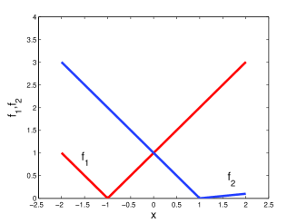
where α(0,1)𝛼01\alpha\in(0,1) (see also Figure 1). For simplicity we assume that ϵ=(ϵ¯,ϵ¯)+2italic-ϵ¯italic-ϵ¯italic-ϵsuperscriptsubscript2\epsilon=(\bar{\epsilon},\bar{\epsilon})\in\mathbbm{R}_{+}^{2}. It is PQ=[1,1]subscript𝑃𝑄11P_{Q}=[-1,1] with

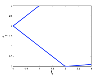
F(1)=(0,2),F(1)=(2,0)formulae-sequence𝐹102𝐹120F(-1)=(0,2),\qquad F(1)=(2,0) (20)

Further, it is

F(1ϵ¯)=(ϵ¯,2+ϵ¯),F(1+ϵ¯α)=(2+ϵ¯α,ϵ¯)formulae-sequence𝐹1¯italic-ϵ¯italic-ϵ2¯italic-ϵ𝐹1¯italic-ϵ𝛼2¯italic-ϵ𝛼¯italic-ϵF(-1-\bar{\epsilon})=(\bar{\epsilon},2+\bar{\epsilon}),\qquad F(1+\frac{\bar{\epsilon}}{\alpha})=(2+\frac{\bar{\epsilon}}{\alpha},\bar{\epsilon}) (21)

Using this and some monoticity arguments on f1subscript𝑓1f_{1} and f2subscript𝑓2f_{2} we see that

PQ,ϵ=(1ϵ¯,1+ϵ¯α]subscript𝑃𝑄italic-ϵ1¯italic-ϵ1¯italic-ϵ𝛼P_{Q,\epsilon}=\left(-1-\bar{\epsilon},1+\frac{\bar{\epsilon}}{\alpha}\right] (22)

Since F(1+ϵ¯+Δα)=(2+ϵ¯+Δα,ϵ¯+Δ)𝐹1¯italic-ϵΔ𝛼2¯italic-ϵΔ𝛼¯italic-ϵΔF(1+\frac{\bar{\epsilon}+\Delta}{\alpha})=(2+\frac{\bar{\epsilon}+\Delta}{\alpha},\bar{\epsilon}+\Delta) it follows that

dist(F(PQ,ϵ+1Δ),F(PQ,ϵ))=Δα,𝑑𝑖𝑠𝑡𝐹subscript𝑃𝑄italic-ϵ1Δ𝐹subscript𝑃𝑄italic-ϵΔ𝛼dist(F(P_{Q,\epsilon+1\Delta}),F(P_{Q,\epsilon}))=\frac{\Delta}{\alpha}, (23)

which can get large for small values of α𝛼\alpha.

Refer to caption
(a) Parameter space
Refer to caption
(b) Image space
Figure 1: Example of MOP (19) for α=0.1𝛼0.1\alpha=0.1.

4 Bounds on the Archive Sizes

Here we give an upper bound U𝑈U on the size of the limit archive obtained by the novel strategy, and discuss that the order of U𝑈U is already optimal.

Theorem 4.1

Let ϵ+kitalic-ϵsuperscriptsubscript𝑘\epsilon\in\mathbbm{R}_{+}^{k}, Δ,Δ+superscriptΔΔsubscript\Delta^{*},\Delta\in\mathbbm{R}_{+} with Δ<ΔsuperscriptΔΔ\Delta^{*}<\Delta be given. Further let mi=minxQfi(x)subscript𝑚𝑖subscript𝑥𝑄subscript𝑓𝑖𝑥m_{i}=\min_{x\in Q}f_{i}(x) and Mi=maxxQfi(x),subscript𝑀𝑖subscript𝑥𝑄subscript𝑓𝑖𝑥M_{i}=\max_{x\in Q}f_{i}(x), 1ik1𝑖𝑘1\leq i\leq k, and l0subscript𝑙0l_{0} as in Theorem 3.2. Then, when using 𝐴𝑟𝑐ℎ𝑖𝑣𝑒𝑈𝑝𝑑𝑎𝑡𝑒𝑃Q,ϵsubscript𝐴𝑟𝑐ℎ𝑖𝑣𝑒𝑈𝑝𝑑𝑎𝑡𝑒𝑃𝑄italic-ϵ\mathit{ArchiveUpdateP_{Q,\epsilon}}, the archive size maintained in Algorithm 1 for all ll0𝑙subscript𝑙0l\geq l_{0} is bounded as

|Al|(1Δ)ki=1k(ϵi+2Δ+Δ)j=1jik(Mjmj+Δ).subscript𝐴𝑙superscript1superscriptΔ𝑘superscriptsubscript𝑖1𝑘subscriptitalic-ϵ𝑖2ΔsuperscriptΔsuperscriptsubscriptproductFRACOP𝑗1𝑗𝑖𝑘subscript𝑀𝑗subscript𝑚𝑗superscriptΔ|A_{l}|\leq\left(\frac{1}{\Delta^{*}}\right)^{k}\sum\limits_{i=1}^{k}(\epsilon_{i}+2\Delta+\Delta^{*})\prod\limits_{j=1\atop j\neq i}^{k}(M_{j}-m_{j}+\Delta^{*}). (24)
Proof.

Let ll0𝑙subscript𝑙0l\geq l_{0} and the archive Alsubscript𝐴𝑙A_{l} be given. Since AlPQ,ϵ+2Δsubscript𝐴𝑙subscript𝑃𝑄italic-ϵ2ΔA_{l}\subset P_{Q,\epsilon+2\Delta} (see Theorem 3.2) we are interested in an upper bound on the volume of F(PQ,ϵ+2Δ)𝐹subscript𝑃𝑄italic-ϵ2ΔF(P_{Q,\epsilon+2\Delta}). For this, we consider first the (k1)𝑘1(k-1)-dimensional volume of the Pareto front F(PQ)𝐹subscript𝑃𝑄F(P_{Q}). Due to the nature of nondominance we can assume that F(PQ)𝐹subscript𝑃𝑄F(P_{Q}) is located in the graph of a map

Φf:KkΦf(u1,,uk1)=(u1,,uk1,f(u1,,uk1)),:subscriptΦ𝑓𝐾superscript𝑘subscriptΦ𝑓subscript𝑢1subscript𝑢𝑘1subscript𝑢1subscript𝑢𝑘1𝑓subscript𝑢1subscript𝑢𝑘1\begin{split}\Phi_{f}&:K\to\mathbbm{R}^{k}\\ \Phi_{f}(u_{1},\ldots,u_{k-1})&=(u_{1},\ldots,u_{k-1},f(u_{1},\ldots,u_{k-1})),\end{split} (25)

where K:=[m1,M1]××[mk1,Mk1]assign𝐾subscript𝑚1subscript𝑀1subscript𝑚𝑘1subscript𝑀𝑘1K:=[m_{1},M_{1}]\times\ldots\times[m_{k-1},M_{k-1}] and f:K[mk,Mk]:𝑓𝐾subscript𝑚𝑘subscript𝑀𝑘f:K\to[m_{k},M_{k}] which satisfies the monotonicity conditions

f(u1,,ui1,xi,ui+1,,uk1)f(u1,,ui1,yi,ui+1,,uk1)i=1,,k1,uj[mj,Mj],j=1,,i1,i+1,,k1,xi,yi[mi,Mi],xiyi.formulae-sequence𝑓subscript𝑢1subscript𝑢𝑖1subscript𝑥𝑖subscript𝑢𝑖1subscript𝑢𝑘1𝑓subscript𝑢1subscript𝑢𝑖1subscript𝑦𝑖subscript𝑢𝑖1subscript𝑢𝑘1for-all𝑖1𝑘1subscript𝑢𝑗subscript𝑚𝑗subscript𝑀𝑗formulae-sequence𝑗1𝑖1𝑖1𝑘1subscript𝑥𝑖formulae-sequencesubscript𝑦𝑖subscript𝑚𝑖subscript𝑀𝑖subscript𝑥𝑖subscript𝑦𝑖\begin{split}f(u_{1},\ldots,u_{i-1},x_{i},u_{i+1},\ldots,u_{k-1})\leq f(u_{1},\ldots,u_{i-1},y_{i},u_{i+1},\ldots,u_{k-1})\\ \forall i=1,\ldots,k-1,\\ u_{j}\in[m_{j},M_{j}],j=1,\ldots,i-1,i+1,\ldots,k-1,\\ x_{i},y_{i}\in[m_{i},M_{i}],x_{i}\leq y_{i}.\end{split} (26)

Further, we can assume that f𝑓f is sufficiently smooth. If not, we can replace f𝑓f by a smooth function f~~𝑓\tilde{f} such that the volume of Φf~subscriptΦ~𝑓\Phi_{\tilde{f}} is larger than the volume of ΦfsubscriptΦ𝑓\Phi_{f} as the following discussion shows:
if f(mi,,mk1)=mk𝑓subscript𝑚𝑖subscript𝑚𝑘1subscript𝑚𝑘f(m_{i},\ldots,m_{k-1})=m_{k}, the Pareto front consists of one point, F(PQ)={(m1,,mk)}𝐹subscript𝑃𝑄subscript𝑚1subscript𝑚𝑘F(P_{Q})=\left\{(m_{1},\ldots,m_{k})\right\}, and has minimal volume 00. Since we are interested in upper bounds on the volume we can omit this case. Doing so, a smooth function f~:K[mk,Mk]:~𝑓𝐾subscript𝑚𝑘subscript𝑀𝑘\tilde{f}:K\to[m_{k},M_{k}] exists with f~(x)f(x),xKformulae-sequence~𝑓𝑥𝑓𝑥for-all𝑥𝐾\tilde{f}(x)\leq f(x),\,\forall x\in K that fulfills the monotonicity conditions (26). The (k1)𝑘1(k-1)-dimensional volume of Φf~subscriptΦ~𝑓\Phi_{\tilde{f}} is obviously larger than the volume of ΦfsubscriptΦ𝑓\Phi_{f}. Under the smoothness assumption we can replace condition (26) by

fuiu0,uK,i=1,,k1.formulae-sequence𝑓subscript𝑢𝑖𝑢0formulae-sequencefor-all𝑢𝐾for-all𝑖1𝑘1\frac{\partial f}{\partial u_{i}}u\leq 0,\quad\forall u\in K,\;\forall i=1,\ldots,k-1. (27)

The (k1)𝑘1(k-1)-dimensional volume of ΦfsubscriptΦ𝑓\Phi_{f} with parameter range K𝐾K is given by (see [5]):

Volk1(Φf)=Kf2+1𝑑u,𝑉𝑜subscript𝑙𝑘1subscriptΦ𝑓subscript𝐾superscriptnorm𝑓21differential-d𝑢Vol_{k-1}(\Phi_{f})=\int_{K}\sqrt{||\nabla f||^{2}+1}du, (28)

where f𝑓\nabla f denotes the gradient of f𝑓f. Analogue to [14] (see also Appendix 1) the volume can be estimated by using partial integration and the monotonicity conditions (27) by:

Volk1(Φf)i=1kj=1jik(Mjmj).𝑉𝑜subscript𝑙𝑘1subscriptΦ𝑓superscriptsubscript𝑖1𝑘superscriptsubscriptproductFRACOP𝑗1𝑗𝑖𝑘subscript𝑀𝑗subscript𝑚𝑗Vol_{k-1}(\Phi_{f})\leq\sum\limits_{i=1}^{k}\prod\limits_{j=1\atop j\neq i}^{k}(M_{j}-m_{j}). (29)

Considering this and the nature of ϵitalic-ϵ-\epsilon-dominance we can bound the k𝑘k-dimensional volume of F(PQ,ϵ+2Δ)𝐹subscript𝑃𝑄italic-ϵ2ΔF(P_{Q,\epsilon+2\Delta}) by:

Volk(F(PQ,ϵ+2Δ))i=1k(ϵi+2Δ)j=1jik(Mjmj),𝑉𝑜subscript𝑙𝑘𝐹subscript𝑃𝑄italic-ϵ2Δsuperscriptsubscript𝑖1𝑘subscriptitalic-ϵ𝑖2ΔsuperscriptsubscriptproductFRACOP𝑗1𝑗𝑖𝑘subscript𝑀𝑗subscript𝑚𝑗Vol_{k}(F(P_{Q,\epsilon+2\Delta}))\leq\sum\limits_{i=1}^{k}(\epsilon_{i}+2\Delta)\prod\limits_{j=1\atop j\neq i}^{k}(M_{j}-m_{j}), (30)

Since F(a1)F(a2)Δnorm𝐹subscript𝑎1𝐹subscript𝑎2superscriptΔ\|F(a_{1})-F(a_{2})\|\geq\Delta^{*} for all a1,a2Alsubscript𝑎1subscript𝑎2subscript𝐴𝑙a_{1},a_{2}\in A_{l} it follows that the boxes

B12Δ(F(a)),aAl,superscriptsubscript𝐵12superscriptΔ𝐹𝑎𝑎subscript𝐴𝑙B_{\frac{1}{2}\Delta^{*}}^{\infty}(F(a)),\quad a\in A_{l}, (31)

are mutually nonoverlapping. Further, if F(a)F(PQ,ϵ+2Δ)𝐹𝑎𝐹subscript𝑃𝑄italic-ϵ2ΔF(a)\in F(P_{Q,\epsilon+2\Delta}), then B12Δ(F(a))superscriptsubscript𝐵12superscriptΔ𝐹𝑎B_{\frac{1}{2}\Delta^{*}}^{\infty}(F(a)) is included in a Δ/2superscriptΔ2\Delta^{*}/2-neighborhood F~~𝐹\tilde{F} of F(PQ,ϵ+2Δ)𝐹subscript𝑃𝑄italic-ϵ2ΔF(P_{Q,\epsilon+2\Delta}) with

Volk(F~)i=1k(ϵi+2Δ+Δ)j=1jik(Mjmj+Δ).𝑉𝑜subscript𝑙𝑘~𝐹superscriptsubscript𝑖1𝑘subscriptitalic-ϵ𝑖2ΔsuperscriptΔsuperscriptsubscriptproductFRACOP𝑗1𝑗𝑖𝑘subscript𝑀𝑗subscript𝑚𝑗superscriptΔVol_{k}(\tilde{F})\leq\sum\limits_{i=1}^{k}(\epsilon_{i}+2\Delta+\Delta^{*})\prod\limits_{j=1\atop j\neq i}^{k}(M_{j}-m_{j}+\Delta^{*}). (32)

The maximal number of entries in Alsubscript𝐴𝑙A_{l} can now be estimated by

|Al|Volk(F~)Volk(B12Δ(F(a))),subscript𝐴𝑙𝑉𝑜subscript𝑙𝑘~𝐹𝑉𝑜subscript𝑙𝑘superscriptsubscript𝐵12superscriptΔ𝐹𝑎|A_{l}|\leq\frac{Vol_{k}(\tilde{F})}{Vol_{k}(B_{\frac{1}{2}\Delta^{*}}^{\infty}(F(a)))}, (33)

and the claim follows since the volume of B12Δ(F(a))superscriptsubscript𝐵12superscriptΔ𝐹𝑎B_{\frac{1}{2}\Delta^{*}}^{\infty}(F(a)) is obviously given by (Δ)ksuperscriptsuperscriptΔ𝑘(\Delta^{*})^{k}. ∎

In particular interesting is certainly the growth of the magnitudes of the (limit) archives for vanishing discretization parameter ΔΔ\Delta. Since for every meaningful computation the value ΔΔ\Delta will be smaller than every entry of ϵitalic-ϵ\epsilon, we can assume ϵi=ciΔsubscriptitalic-ϵ𝑖subscript𝑐𝑖Δ\epsilon_{i}=c_{i}\Delta with ci>1subscript𝑐𝑖1c_{i}>1. Using (24) and for simlicity Δ=ΔΔsuperscriptΔ\Delta=\Delta^{*} we see that

|Al|(1Δ)k1i=1k(ci+3)j=1jik(Mjmj+Δ).subscript𝐴𝑙superscript1Δ𝑘1superscriptsubscript𝑖1𝑘subscript𝑐𝑖3superscriptsubscriptproductFRACOP𝑗1𝑗𝑖𝑘subscript𝑀𝑗subscript𝑚𝑗superscriptΔ|A_{l}|\leq\left(\frac{1}{\Delta}\right)^{k-1}\sum\limits_{i=1}^{k}(c_{i}+3)\prod\limits_{j=1\atop j\neq i}^{k}(M_{j}-m_{j}+\Delta^{*}). (34)

Thus, the growth of the magnitudes is of order 𝒪((1Δ)k1)𝒪superscript1Δ𝑘1\mathcal{O}\left(\left(\frac{1}{\Delta}\right)^{k-1}\right) for Δ0Δ0\Delta\to 0. Regarding the fact that PQsubscript𝑃𝑄P_{Q}, which is contained in PQ,ϵsubscript𝑃𝑄italic-ϵP_{Q,\epsilon} for all values of ϵ+kitalic-ϵsuperscriptsubscript𝑘\epsilon\in\mathbbm{R}_{+}^{k}, typically forms a (k1)𝑘1(k-1)-dimensional object, we see that the order of the magnitude of the archive with respect to ΔΔ\Delta is already optimal. This is due to the fact that the discretization (line 3 of Algorithm 2) is realized in image space. An analogue result for a discretization in parameter space, however, can not hold since PQ,ϵsubscript𝑃𝑄italic-ϵP_{Q,\epsilon} is n𝑛n-dimensional.

Remark 4.2

In case the algorithm is modified as described in Remark 3.3 (c), the upper bound for the magnitude of the archive is given by

|Alx|(1Δ+1)nj=1n(biai),superscriptsubscript𝐴𝑙𝑥superscript1superscriptΔ1𝑛superscriptsubscriptproduct𝑗1𝑛subscript𝑏𝑖subscript𝑎𝑖|A_{l}^{x}|\leq\left(\frac{1}{\Delta^{*}}+1\right)^{n}\prod_{j=1}^{n}(b_{i}-a_{i}), (35)

where Q[a1,b1]××[an,bn]𝑄subscript𝑎1subscript𝑏1subscript𝑎𝑛subscript𝑏𝑛Q\subset[a_{1},b_{1}]\times\ldots\times[a_{n},b_{n}] (PQ,ϵ+2Δsubscript𝑃𝑄italic-ϵ2ΔP_{Q,\epsilon+2\Delta} is certainly included in [a1,b1]××[an,bn]subscript𝑎1subscript𝑏1subscript𝑎𝑛subscript𝑏𝑛[a_{1},b_{1}]\times\ldots\times[a_{n},b_{n}], and maximal 1/Δ+11superscriptΔ11/\Delta^{*}+1 elements can be placed in each coordinate direction). To see that this bound is tight we consider the example

F:[0,1]nk,F(x)c0k,:𝐹formulae-sequencesuperscript01𝑛superscript𝑘𝐹𝑥subscript𝑐0superscript𝑘F:[0,1]^{n}\to\mathbbm{R}^{k},\quad F(x)\equiv c_{0}\in\mathbbm{R}^{k}, (36)

and let Δ=1/s,sformulae-sequenceΔ1𝑠𝑠\Delta=1/s,\;s\in\mathbbm{N}. Define xi1,,in=(i1Δ,,inΔ)subscript𝑥subscript𝑖1subscript𝑖𝑛subscript𝑖1Δsubscript𝑖𝑛Δx_{i_{1},\ldots,i_{n}}=(i_{1}\Delta,\ldots,i_{n}\Delta) and

𝒟:={xi1,,in|0i1,,ins}.assign𝒟conditional-setsubscript𝑥subscript𝑖1subscript𝑖𝑛formulae-sequence0subscript𝑖1subscript𝑖𝑛𝑠\mathcal{D}:=\left\{x_{i_{1},\ldots,i_{n}}|0\leq i_{1},\ldots,i_{n}\leq s\right\}. (37)

Since 𝒟[0,1]n𝒟superscript01𝑛\mathcal{D}\subset[0,1]^{n} and d(z1,z2)Δ>Δsubscript𝑑subscript𝑧1subscript𝑧2ΔsuperscriptΔd_{\infty}(z_{1},z_{2})\geq\Delta>\Delta^{*} for all z1,z2𝒟subscript𝑧1subscript𝑧2𝒟z_{1},z_{2}\in\mathcal{D}, z1z2subscript𝑧1subscript𝑧2z_{1}\neq z_{2}, all points in 𝒟𝒟\mathcal{D} will be accepted by the archiver (assuming that only points z𝒟𝑧𝒟z\in\mathcal{D} are inserted) leading to an archive A𝐴A with |A|=|𝒟|=(s+1)n𝐴𝒟superscript𝑠1𝑛|A|=|\mathcal{D}|=(s+1)^{n}.
Since PQ,ϵsubscript𝑃𝑄italic-ϵP_{Q,\epsilon} is n𝑛n-dimensional, the growth of the magnitudes of the archives is also beyond this constructed example of order 𝒪((1Δ)n)𝒪superscript1Δ𝑛\mathcal{O}\left(\left(\frac{1}{\Delta}\right)^{n}\right) for Δ0Δ0\Delta\to 0. This makes a huge difference to the other archiver since for general MOPs we have nkmuch-greater-than𝑛𝑘n\gg k.

5 Numerical Results

Here we demonstrate the practicability of the novel archiver on five examples. For this, we run and compare ArchiveUpdatePQ,ϵ𝐴𝑟𝑐𝑖𝑣𝑒𝑈𝑝𝑑𝑎𝑡𝑒subscript𝑃𝑄italic-ϵArchiveUpdateP_{Q,\epsilon} for different values of ΔΔ\Delta including Δ0=0subscriptΔ00\Delta_{0}=0, which is the archiver which accepts all test points which are not ϵitalic-ϵ-\epsilon dominated by any other test point (see Remark 4.3 (a)). To obtain a fair comparison we have decided to take a random search operator for the generation process (the same sequence of points for all settings). An implementation of the archiver including these examples can be found in [1].

5.1 Example 1

First we consider the MOP suggested by Tanaka ([16]):

F:22,F(x1,x2)=(x1,x2):𝐹formulae-sequencesuperscript2superscript2𝐹subscript𝑥1subscript𝑥2subscript𝑥1subscript𝑥2F:\mathbbm{R}^{2}\to\mathbbm{R}^{2},\quad F(x_{1},x_{2})=(x_{1},x_{2}) (38)

where

C1(x)=x12+x2210.1cos(16arctan(x1/x2))0C2(x)=(x10.5)2+(x20.5)20.5subscript𝐶1𝑥superscriptsubscript𝑥12superscriptsubscript𝑥2210.116subscript𝑥1subscript𝑥20subscript𝐶2𝑥superscriptsubscript𝑥10.52superscriptsubscript𝑥20.520.5\begin{split}C_{1}(x)&=x_{1}^{2}+x_{2}^{2}-1-0.1\cos(16\arctan(x_{1}/x_{2}))\geq 0\\ C_{2}(x)&=(x_{1}-0.5)^{2}+(x_{2}-0.5)^{2}\leq 0.5\end{split}

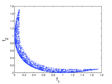
Figure 2 shows a numerical result for N=200,000𝑁200000N=200,000 randomly chosen points within Q=[0,π]2𝑄superscript0𝜋2Q=[0,\pi]^{2} and for three different values of the discretization parameter: Δ0=0subscriptΔ00\Delta_{0}=0, Δ1=0.01subscriptΔ10.01\Delta_{1}=0.01 and Δ2=0.05subscriptΔ20.05\Delta_{2}=0.05. As anticipated, the granularity of the resulting archive increases with the value of ΔΔ\Delta. Thus, the approximation quality decreases, but also the running time of the algorithm (see Table 1).

Refer to caption
(a) Δ0=0,|Afinal|=3824formulae-sequencesubscriptΔ00subscript𝐴𝑓𝑖𝑛𝑎𝑙3824\Delta_{0}=0,\quad|A_{final}|=3824
Refer to caption
(b) Delta1=0.01,|Afinal|=834formulae-sequence𝐷𝑒𝑙𝑡subscript𝑎10.01subscript𝐴𝑓𝑖𝑛𝑎𝑙834Delta_{1}=0.01,\quad|A_{final}|=834
Refer to caption
(c) Delta2=0.05,|Afinal|=73formulae-sequence𝐷𝑒𝑙𝑡subscript𝑎20.05subscript𝐴𝑓𝑖𝑛𝑎𝑙73Delta_{2}=0.05,\quad|A_{final}|=73
Figure 2: Results for MOP (38) for different values of ΔΔ\Delta leading to different granularities of the approximation.
Table 1: Comparison of the magnitudes of the final archive (|Afinal|subscript𝐴𝑓𝑖𝑛𝑎𝑙|A_{final}|, rounded) and the corresponding update times (T𝑇T, in seconds) for MOP (38) and for different values of ΔΔ\Delta. We have taken the average result of 100 test runs.
ΔΔ\Delta |Afinal|subscript𝐴𝑓𝑖𝑛𝑎𝑙|A_{final}| T𝑇T
00 3836 32.98
0.010.010.01 827 6.22
0.050.050.05 68 1.80

5.2 Example 2

Next, we consider the following MOP proposed in [10]:

F:22F(x1,x2)=((x1t1(c+2a)+a)2+(x2t2b)2(x1t1(c+2a)a)2+(x2t2b)2),:𝐹superscript2superscript2𝐹subscript𝑥1subscript𝑥2fragments(x1t1(c2a)a)2(x2t2b)2fragments(x1t1(c2a)a)2(x2t2b)2\begin{split}F&:\mathbbm{R}^{2}\to\mathbbm{R}^{2}\\ F(x_{1},x_{2})&=\left(\begin{tabular}[]{c}$(x_{1}-t_{1}(c+2a)+a)^{2}+(x_{2}-t_{2}b)^{2}$\\ $(x_{1}-t_{1}(c+2a)-a)^{2}+(x_{2}-t_{2}b)^{2}$\end{tabular}\right),\end{split} (39)

where

t1=sgn(x1)min(|x1|ac/22a+c,1),t2=sgn(x2)min(|x2|b/2b,1).formulae-sequencesubscript𝑡1sgnsubscript𝑥1subscript𝑥1𝑎𝑐22𝑎𝑐1subscript𝑡2sgnsubscript𝑥2subscript𝑥2𝑏2𝑏1t_{1}=\mbox{sgn}(x_{1})\min\left(\left\lceil\frac{|x_{1}|-a-c/2}{2a+c}\right\rceil,1\right),t_{2}=\mbox{sgn}(x_{2})\min\left(\left\lceil\frac{|x_{2}|-b/2}{b}\right\rceil,1\right).

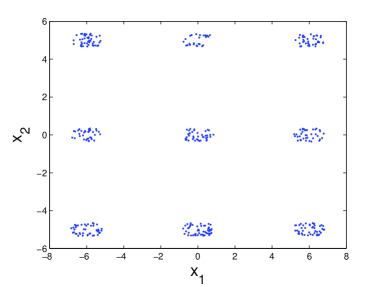
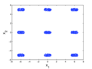
The Pareto set consists of nine connected components of length a𝑎a with identical images. We have chosen the values a=0.5𝑎0.5a=0.5, b=c=5𝑏𝑐5b=c=5, ϵ=(0.1,0.1)italic-ϵ0.10.1\epsilon=(0.1,0.1), and the domain as Q=[20,20]2𝑄superscript20202Q=[-20,20]^{2}. Figure 3 shows some numerical results for N=100,000𝑁100000N=100,000 randomly chosen points within Q𝑄Q and for the three variants of the archiver ArchiveUpdatePQ,ϵ𝐴𝑟𝑐𝑖𝑣𝑒𝑈𝑝𝑑𝑎𝑡𝑒subscript𝑃𝑄italic-ϵArchiveUpdateP_{Q,\epsilon}: (a) Δ=(0,0)Δ00\Delta=(0,0), i.e., the archiver which aims to store the entire set PQ,ϵsubscript𝑃𝑄italic-ϵP_{Q,\epsilon}, (b) a discretization (in image space) using Δ=(0.02,0.02)Δ0.020.02\Delta=(0.02,0.02), and (c) the variant which is described in Remark 3.3 (c) using Δx=(0.1,0.1)subscriptΔ𝑥0.10.1\Delta_{x}=(0.1,0.1) for a discretization of the parameter space. As anticipated, the solution in (b) is more uniform in image space compared to the solution in (c), which is, in turn, more uniform in parameter space. Note that the solution in (b), i.e., where the discretization has been done in image space, already ’detects’ all nine connected components in parameter space. This is certainly due to the fact that the search has been done by selecting random points wich are uniformly distributed within Q𝑄Q. One interesting point for future studies would be to investigate if this capability still holds when other search strategies are chosen (which include, e.g., local search strategies).
Refer to caption
Refer to caption
(a) Δ=(0,0)Δ00\Delta=(0,0), |Afinal|=2150subscript𝐴𝑓𝑖𝑛𝑎𝑙2150|A_{final}|=2150
Refer to caption
Refer to caption
(b) Δ=(0.02,0.02)Δ0.020.02\Delta=(0.02,0.02), |Afinal|=365subscript𝐴𝑓𝑖𝑛𝑎𝑙365|A_{final}|=365
Refer to caption
Refer to caption
(c) Δx=(0.1,0.1)subscriptΔ𝑥0.10.1\Delta_{x}=(0.1,0.1), |Afinal|=410subscript𝐴𝑓𝑖𝑛𝑎𝑙410|A_{final}|=410
Figure 3: Numerical results for MOP (39) for the three different variants of ArchiveUpdatePQ,ϵ𝐴𝑟𝑐𝑖𝑣𝑒𝑈𝑝𝑑𝑎𝑡𝑒subscript𝑃𝑄italic-ϵArchiveUpdateP_{Q,\epsilon}.

5.3 Example 3

Finally, we consider the production model proposed in [12]:

f1,f2:n:subscript𝑓1subscript𝑓2superscript𝑛f_{1},f_{2}:\mathbbm{R}^{n}\to\mathbbm{R},

f1(x)=j=1nxj,f2(x)=1j=1n(1wj(xj)),formulae-sequencesubscript𝑓1𝑥superscriptsubscript𝑗1𝑛subscript𝑥𝑗subscript𝑓2𝑥1superscriptsubscriptproduct𝑗1𝑛1subscript𝑤𝑗subscript𝑥𝑗\begin{split}f_{1}(x)&=\sum_{j=1}^{n}x_{j},\\ f_{2}(x)&=1-\prod_{j=1}^{n}(1-w_{j}(x_{j})),\end{split} (40)

where

wj(z)={0.01exp((z20)2.5)forj=1,20.01exp(z15)for3jnsubscript𝑤𝑗𝑧cases0.01superscript𝑧202.5formulae-sequencefor𝑗120.01𝑧15for3𝑗𝑛\displaystyle w_{j}(z)=\left\{\begin{array}[]{l@{\quad}l}0.01\cdot\exp(-(\frac{z}{20})^{2.5})&\quad\mbox{for}\quad j=1,2\\[5.69054pt] 0.01\cdot\exp(-\frac{z}{15})&\quad\mbox{for}\quad 3\leq j\leq n\end{array}\right.

The two objective functions have to be interpreted as follows. f1subscript𝑓1f_{1} represents the sum of the additional cost necessary for a more reliable production of n𝑛n items. These items are needed for the composition of a certain product. The function f2subscript𝑓2f_{2} describes the total failure rate for the production of this composed product.
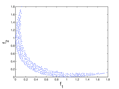
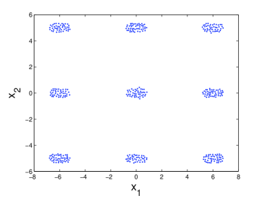
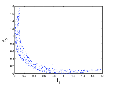
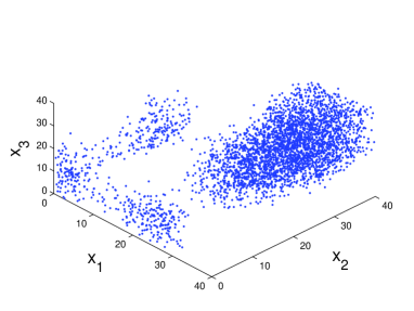
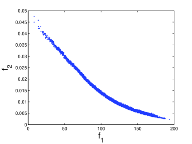
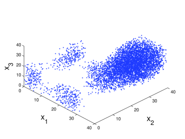
Here we have chosen n=5𝑛5n=5, Q=[0,40]n𝑄superscript040𝑛Q=[0,40]^{n}, and ϵ=(0.1,0.001)italic-ϵ0.10.001\epsilon=(0.1,0.001) which corresponds to 101010 percent of one cost unit for one item (ϵ1subscriptitalic-ϵ1\epsilon_{1}), and to 0.10.10.1 percent of the total failure rate (ϵ2subscriptitalic-ϵ2\epsilon_{2}). Figure 4 shows numerical results for (a) Δ=(0,0)Δ00\Delta=(0,0) and (b) for Δ=ϵ/3Δitalic-ϵ3\Delta=\epsilon/3. Note the symmetries in the model: it is e.g., F(x1,x2,)=F(x2,x1,)𝐹subscript𝑥1subscript𝑥2𝐹subscript𝑥2subscript𝑥1F(x_{1},x_{2},\ldots)=F(x_{2},x_{1},\ldots) by which is follows that the two connected components at x1=0subscript𝑥10x_{1}=0 and x2=0subscript𝑥20x_{2}=0 (see Figure 4 (a)) have the same image. Also in this case the archiver detects both components though the discretization has been done in image space (Figure 4 (b)).
Refer to caption
Refer to caption
(a) Δ=(0,0)Δ00\Delta=(0,0), |Afinal|=5939subscript𝐴𝑓𝑖𝑛𝑎𝑙5939|A_{final}|=5939
Refer to caption
Refer to caption
(b) Δ=(0.033,0.00033)Δ0.0330.00033\Delta=(0.033,0.00033), |Afinal|=3544subscript𝐴𝑓𝑖𝑛𝑎𝑙3544|A_{final}|=3544
Figure 4: Numerical result for MOP (40): projections to the coordinates x1,x2,x3subscript𝑥1subscript𝑥2subscript𝑥3x_{1},x_{2},x_{3} of the final archive (left) and their images (right).

5.4 Example 4

Next, we consider a real-life engineering problem, namely the design of a four-bar plane truss ([15]):

F:42f1(x)=L(2x1+2x2+2x3+x4)f2(x)=FLE(2x1+22x222x3+1x4):𝐹superscript4superscript2subscript𝑓1𝑥𝐿2subscript𝑥12subscript𝑥22subscript𝑥3subscript𝑥4subscript𝑓2𝑥𝐹𝐿𝐸2subscript𝑥122subscript𝑥222subscript𝑥31subscript𝑥4\begin{split}F&:\mathbbm{R}^{4}\to\mathbbm{R}^{2}\\ f_{1}(x)&=L(2x_{1}+\sqrt{2}x_{2}+\sqrt{2}x_{3}+x_{4})\\ f_{2}(x)&=\frac{FL}{E}\left(\frac{2}{x_{1}}+\frac{2\sqrt{2}}{x_{2}}-\frac{2\sqrt{2}}{x_{3}}+\frac{1}{x_{4}}\right)\end{split} (42)

f1subscript𝑓1f_{1} models the volume of the truss, and f2subscript𝑓2f_{2} the displacement of the joint. The model constants are the length L𝐿L of each bar (L=200𝐿200L=200 cm), the elasticity constants E𝐸E and σ𝜎\sigma of the materials involved (E=2×10⁵𝐸2superscript105E=2\times 10^{5} kN/cm3, σ=10𝜎10\sigma=10 kN/cm2), and the force F𝐹F which causes the stress of the truss (F=10𝐹10F=10 kN). The parameters xisubscript𝑥𝑖x_{i} represent the cross sectional areas of the four bars of the truss. The physical restrictions are given by

Q=[F/σ,3F/σ]×[2F/σ,3F/σ]2×[F/σ,3F/σ]𝑄𝐹𝜎3𝐹𝜎superscript2𝐹𝜎3𝐹𝜎2𝐹𝜎3𝐹𝜎Q=[F/\sigma,3F/\sigma]\times[\sqrt{2}F/\sigma,3F/\sigma]^{2}\times[F/\sigma,3F/\sigma] (43)

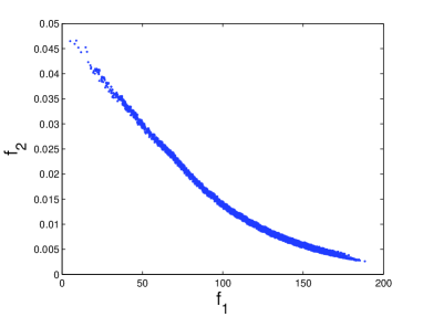
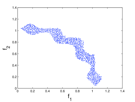
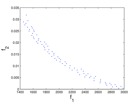
For the allowed tolerances we follow the suggestion made in [4] and set ϵ1=50subscriptitalic-ϵ150\epsilon_{1}=50 cm3 and ϵ2=0.0005subscriptitalic-ϵ20.0005\epsilon_{2}=0.0005 cm. Figure 5 shows a result for N=500,000𝑁500000N=500,000 randomly chosen points within Q𝑄Q and for Δ=(10,0.0001)Δ100.0001\Delta=(10,0.0001), i.e., Δi=ϵi/5subscriptΔ𝑖subscriptitalic-ϵ𝑖5\Delta_{i}=\epsilon_{i}/5 (see Remark 4.3 (b)). The final archive consists of 78 elements, and the computational time was 5.5 seconds. In contrast, a run of the same algorithm with the same setting but with Δ=0Δ0\Delta=0 took 4 minutes and 21 seconds leading to an archive with 8377 elements.
Refer to caption
Figure 5: Numerical result for MOP (42). Here, we have chosen ϵ=(50,0.0005)italic-ϵ500.0005\epsilon=(50,0.0005) and Δ=(10,0.0001)Δ100.0001\Delta=(10,0.0001).

5.5 Example 5

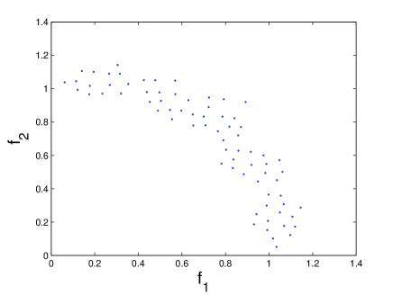
Finally, we consider a bi-objective {0,1}-knapsack problem which should demonstrate that the additional consideration of approximate solutions can be beneficial for the decision maker.

f1,f2:{0,1}n,f1(x)=j=1ncj1xj,f2(x)=j=1ncj2xj:subscript𝑓1subscript𝑓2formulae-sequencesuperscript01𝑛formulae-sequencesubscript𝑓1𝑥superscriptsubscript𝑗1𝑛superscriptsubscript𝑐𝑗1subscript𝑥𝑗subscript𝑓2𝑥superscriptsubscript𝑗1𝑛superscriptsubscript𝑐𝑗2subscript𝑥𝑗f_{1},f_{2}:\{0,1\}^{n}\to\mathbbm{R},\ f_{1}(x)=\sum\limits_{j=1}^{n}c_{j}^{1}x_{j},\ f_{2}(x)=\sum\limits_{j=1}^{n}c_{j}^{2}x_{j} (44)

s.t.

j=1nwjxjW,xj{0,1},j=1,,n,formulae-sequencesuperscriptsubscript𝑗1𝑛subscript𝑤𝑗subscript𝑥𝑗𝑊formulae-sequencesubscript𝑥𝑗01𝑗1𝑛\sum\limits_{j=1}^{n}w_{j}x_{j}\leq W,\ x_{j}\in\{0,1\},\;j=1,\ldots,n,

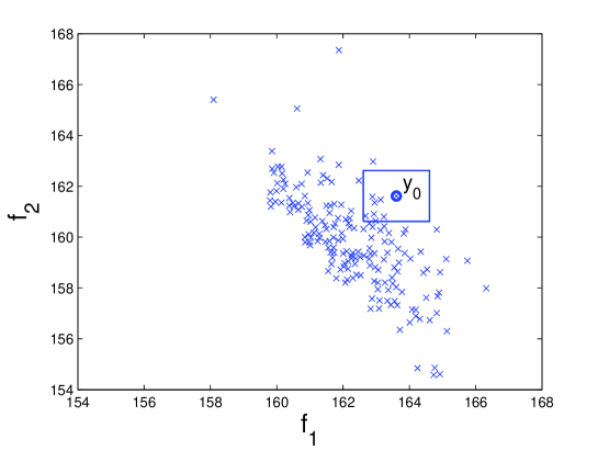
where cjisuperscriptsubscript𝑐𝑗𝑖c_{j}^{i} represents the value of item j𝑗j on criterion i,i=1,2formulae-sequence𝑖𝑖12i,i=1,2; xj=1subscript𝑥𝑗1x_{j}=1, j=1,,n𝑗1𝑛j=1,\ldots,n, if item j𝑗j is included in the knapsack, else xj=0subscript𝑥𝑗0x_{j}=0. wjsubscript𝑤𝑗w_{j} is the weight of item j𝑗j, and W𝑊W the overall knapsack capacity. Figure 6 shows one numerical result obtained by an evolutionary strategy222A modification of the algorithm presented in [17] which uses the novel archiver. for an instance with n=30𝑛30n=30 items and with randomly chosen values cji[8,12]superscriptsubscript𝑐𝑗𝑖812c_{j}^{i}\in[8,12], and capacity W=15𝑊15W=15 (note that we are faced with a maximization problem). For ϵ=(2,2)italic-ϵ22\epsilon=(2,2) and Δ=0.1Δ0.1\Delta=0.1 a total of 182 elements forms the final archive, and only six of them are nondominated. When taking, for instance, x0subscript𝑥0x_{0} as reference (assuming, e.g., that this point has been selected by the DM out of the nondominated points) and assuming a tolerance of 1 which represents a possible loss of 0.6%percent0.60.6\% compared to x0subscript𝑥0x_{0} for each objective value, the resulting region of interest includes seven approximate solutions (see Figure 6). These solutions, though similar in objective space, differ significantly in parameter space: two solutions differ compared to x0subscript𝑥0x_{0} in 8 items, one in 10, and 4 solutions differ even in 12 items. Thus, in this case it is obvious that by tolerating approximate solutions – where the loss of them can be determined a priori – a larger variety of possibilities is offered to the DM.
Refer to caption
Figure 6: Numerical result for MOP (42) with ϵ=(2,2)italic-ϵ22\epsilon=(2,2) and Δ=0.1Δ0.1\Delta=0.1. The rectangle defines one possible region of interest around y0=F(x0)subscript𝑦0𝐹subscript𝑥0y_{0}=F(x_{0}) including seven approximate solutions (see text).
Table 2: ..
c1superscript𝑐1c^{1} c2superscript𝑐2c^{2} x0subscript𝑥0x_{0} x1subscript𝑥1x_{1} x2subscript𝑥2x_{2} x3subscript𝑥3x_{3} x4subscript𝑥4x_{4} x5subscript𝑥5x_{5} x6subscript𝑥6x_{6} x7subscript𝑥7x_{7}
1 1 1 1 1 1 0 0
0 0 1 1 0 1 1 0
1 1 0 1 0 1 1 1
1 1 1 1 1 1 0 1
0 1 0 1 1 1 1 1
0 0 1 1 0 0 0 0
0 1 1 0 1 0 1 1
1 0 0 0 1 0 0 0
1 1 1 1 0 1 1 1
0 0 1 0 0 1 1 0
1 0 0 1 1 1 1 1
0 0 0 0 0 0 0 0
1 1 1 1 1 0 0 0
0 0 0 0 0 0 1 0
1 1 0 1 1 0 1 0
1 1 1 1 1 1 1 1
0 1 1 0 0 1 0 1
0 0 0 0 0 0 0 0
1 1 0 1 0 0 1 1
0 0 0 0 0 1 0 1
0 0 0 0 1 0 0 1
1 1 1 0 1 1 1 1
1 0 1 0 1 0 0 0
0 1 1 1 1 1 1 1
1 0 1 0 0 1 1 0
0 0 0 0 0 0 0 0
0 1 0 0 0 0 0 0
1 1 0 1 1 1 0 1
0 0 0 0 0 0 0 0
1 0 1 1 1 0 1 1

6 Conclusion and Future Work

We have proposed and investigated a novel archiving strategy for stochastic search algorithms which allows – under mild assumptions on the generation process – for a finite size approximation of the set PQ,ϵsubscript𝑃𝑄italic-ϵP_{Q,\epsilon} which contains all ϵitalic-ϵ\epsilon-efficient solutions of an MOP within a compact domain Q𝑄Q. We have proven convergence of the algorithm toward a finite size representation of the set of interest in the probabilistic sense, yielding bounds on the approximation quality and the cardinality of the archives. Finally, we have presented some numerical results indicating the usefulness of the approach.
The consideration of approximate solutions certainly leads to a larger variety of possible options to the DM, but, in turn, also to a higher demand on the related decision making process. Thus, the support for this problem could be one focus of future research. Further, it could be interesting to integrate the archiving strategy directly into the stoachastic search process (as e.g. done in [3] for an EMO algorithm) in order to obtain a fast and reliable search procedure.

Acknoledgements

The second author gratefully acknowledges support from CONACyT project no. 45683-Y.

References

  • [1] http://paradiseo.gforge.inria.fr.
  • [2] R. Blanquero and E. Carrizosa. A. d.c. biobjective location model. Journal of Global Optimization, 23(2):569–580, 2002.
  • [3] K. Deb, M. Mohan, and S. Mishra. Evaluating the ϵitalic-ϵ\epsilon-dominated based multi-objective evolutionary algorithm for a quick computation of Pareto-optimal solutions. Evolutionary Computation, 13(4):501–525, 2005.
  • [4] A. Engau and M. M. Wiecek. Generating epsilon-efficient solutions in multiobjective programming. European Journal of Operational Research, 177(3):1566–1579, 2007.
  • [5] O. Forster. Analysis 3. Vieweg, 1984.
  • [6] J. D. Knowles and D. W. Corne. Metaheuristics for Multiobjective Optimisation, volume 535 of Lecture Notes in Economics and Mathematical Systems, chapter Bounded Pareto Archiving: Theory and Practice, pages 39–64. Springer, 2004.
  • [7] M. Laumanns, L. Thiele, K. Deb, and E. Zitzler. Combining convergence and diversity in evolutionary multiobjective optimization. Evolutionary Computation, 10(3):263–282, 2002.
  • [8] P. Loridan. ϵitalic-ϵ\epsilon-solutions in vector minimization problems. Journal of Optimization, Theory and Application, 42:265–276, 1984.
  • [9] Günter Rudolph and Alexandru Agapie. Convergence Properties of Some Multi-Objective Evolutionary Algorithms. In Proceedings of the 2000 Conference on Evolutionary Computation, volume 2, pages 1010–1016, Piscataway, New Jersey, July 2000. IEEE Press.
  • [10] Günter Rudolph, Boris Naujoks, and Mike Preuss. Capabilities of emoa to detect and preserve equivalent pareto subsets. In EMO, pages 36–50, 2006.
  • [11] G. Ruhe and B. Fruhwirt. ϵitalic-ϵ\epsilon-optimality for bicriteria programs and its application to minimum cost flows. Computing, 44:21–34, 1990.
  • [12] S. Schaeffler, R. Schultz, and K. Weinzierl. Stochastic method for the solution of unconstrained vector optimization problems. Journal of Optimization Theory and Applications, 114(1):209–222, 2002.
  • [13] O. Schütze, C. A. Coello Coello, and E.-G. Talbi. Approximating the ϵitalic-ϵ\epsilon-efficient set of an MOP with stochastic search algorithms. In A. Gelbukh and A. F. Kuri Morales, editors, Mexican International Conference on Artificial Intelligence (MICAI-2007), pages 128–138. Springer-Verlag Berlin Heidelberg, 2007.
  • [14] O. Schütze, M. Laumanns, C. A. Coello Coello, M. Dellnitz, and E.-G. Talbi. Convergence of stochastic search algorithms to finite size Pareto set approximations. To appear in Journal of Global Optimization, 2007.
  • [15] W. Stadler and J. Dauer. Multicriteria optimization in engineering: A tutorial and survey. In M. P. Kamat, editor, Structural Optimization: Status and Future, pages 209–249. American Institute of Aeronautics and Astronautics, 1992.
  • [16] M. Tanaka. GA-based decision support system for multi-criteria optimization. In Proceedings of International Conference on Systems, Man and Cybernetics, pages 1556–1561, 1995.
  • [17] E. Tantar, O. Schütze, J. R. Figueira, Carlos A. Coello Coello, and E.-G. Talbi. Computing and selecting ϵitalic-ϵ\epsilon-efficient solutions of {0,1}01\{0,1\}-knapsack problems. To appear in Proceedings of the 19th International Conference on Multiple Criteria Decision Making (MCDM-2008), 2008.
  • [18] D. J. White. Epsilon efficiency. Journal of Optimization Theory and Applications, 49(2):319–337, 1986.
  • [19] D. J. White. Epsilon-dominating solutions in mean-variance portfolio analysis. European Journal of Operational Research, 105(3):457–466, 1998.

7 Appendix 1

Here we show the inequality in (29), which is taken from [14].
Define

K:=[m1,M1]××[mk1,Mk1],K(i):=[m1,M1]××[mi1,Mi1]×[mi+1,Mi+1]××[mk1,Mk1],u(i):=(u1,,ui1,ui+1,,uk1),i=1,,k1.formulae-sequenceassign𝐾subscript𝑚1subscript𝑀1subscript𝑚𝑘1subscript𝑀𝑘1formulae-sequenceassignsubscript𝐾𝑖subscript𝑚1subscript𝑀1subscript𝑚𝑖1subscript𝑀𝑖1subscript𝑚𝑖1subscript𝑀𝑖1subscript𝑚𝑘1subscript𝑀𝑘1formulae-sequenceassignsubscript𝑢𝑖subscript𝑢1subscript𝑢𝑖1subscript𝑢𝑖1subscript𝑢𝑘1𝑖1𝑘1\begin{split}K&:=[m_{1},M_{1}]\times\ldots\times[m_{k-1},M_{k-1}],\\ K_{(i)}&:=[m_{1},M_{1}]\times\ldots\times[m_{i-1},M_{i-1}]\times[m_{i+1},M_{i+1}]\times\ldots\times[m_{k-1},M_{k-1}],\\ u_{(i)}&:=(u_{1},\ldots,u_{i-1},u_{i+1},\ldots,u_{k-1}),\;i=1,\ldots,k-1.\end{split} (45)

Then, the (k1)𝑘1(k-1)-dimensional volume of ΦfsubscriptΦ𝑓\Phi_{f} with parameter range K𝐾K can be bounded as follows:

Volk1(Φf)=Kf2+1𝑑u=K(fu1)2++(fuk1)2+1𝑑uK|fu1|𝑑u++K|fuk1|𝑑u+K1𝑑u=i=1k1(K(i)(miMi|fui|𝑑ui)𝑑u(i))+K1𝑑u=i=1k1(K(i)(miMifui𝑑ui)𝑑u(i))+K1𝑑ui=1kj=1jik(Mjmj).𝑉𝑜subscript𝑙𝑘1subscriptΦ𝑓subscript𝐾superscriptnorm𝑓21differential-d𝑢subscript𝐾superscript𝑓subscript𝑢12superscript𝑓subscript𝑢𝑘121differential-d𝑢subscript𝐾𝑓subscript𝑢1differential-d𝑢subscript𝐾𝑓subscript𝑢𝑘1differential-d𝑢subscript𝐾1differential-d𝑢superscriptsubscript𝑖1𝑘1subscriptsubscript𝐾𝑖superscriptsubscriptsubscript𝑚𝑖subscript𝑀𝑖𝑓subscript𝑢𝑖differential-dsubscript𝑢𝑖differential-dsubscript𝑢𝑖subscript𝐾1differential-d𝑢superscriptsubscript𝑖1𝑘1subscriptsubscript𝐾𝑖superscriptsubscriptsubscript𝑚𝑖subscript𝑀𝑖𝑓subscript𝑢𝑖differential-dsubscript𝑢𝑖differential-dsubscript𝑢𝑖subscript𝐾1differential-d𝑢superscriptsubscript𝑖1𝑘superscriptsubscriptproductFRACOP𝑗1𝑗𝑖𝑘subscript𝑀𝑗subscript𝑚𝑗\displaystyle\begin{split}Vol_{k-1}(\Phi_{f})&=\int_{K}\sqrt{||\nabla f||^{2}+1}du=\int_{K}\sqrt{\left(\frac{\partial f}{\partial u_{1}}\right)^{2}+\ldots+\left(\frac{\partial f}{\partial u_{k-1}}\right)^{2}+1}du\\ &\leq\int_{K}\left|\frac{\partial f}{\partial u_{1}}\right|du+\ldots+\int_{K}\left|\frac{\partial f}{\partial u_{k-1}}\right|du+\int_{K}1du\\ &=\sum_{i=1}^{k-1}\left(\int_{K_{(i)}}\left(\int_{m_{i}}^{M_{i}}\left|\frac{\partial f}{\partial u_{i}}\right|du_{i}\right)du_{(i)}\right)+\int_{K}1du\\ &=\sum_{i=1}^{k-1}\left(\int_{K_{(i)}}\left(-\int_{m_{i}}^{M_{i}}\frac{\partial f}{\partial u_{i}}du_{i}\right)du_{(i)}\right)+\int_{K}1du\\ &\leq\sum\limits_{i=1}^{k}\prod\limits_{j=1\atop j\neq i}^{k}(M_{j}-m_{j}).\end{split} (46)