Distributed Consensus over Wireless Sensor Networks Affected by Multipath Fading

Abstract

The design of sensor networks capable of reaching a consensus on a globally optimal decision test, without the need for a fusion center, is a problem that has received considerable attention in the last years. Many consensus algorithms have been proposed, with convergence conditions depending on the graph describing the interaction among the nodes. In most works, the graph is undirected and there are no propagation delays. Only recently, the analysis has been extended to consensus algorithms incorporating propagation delays. In this work, we propose a consensus algorithm able to converge to a globally optimal decision statistic, using a wideband wireless network, governed by a fairly simple MAC mechanism, where each link is a multipath, frequency-selective, channel. The main contribution of the paper is to derive necessary and sufficient conditions on the network topology and sufficient conditions on the channel transfer functions guaranteeing the exponential convergence of the consensus algorithm to a globally optimal decision value, for any bounded delay condition.

1 Introduction

Distributed algorithms for achieving consensus in wireless sensor networks, without the need for a fusion center, have been the subject of many recent works. Two excellent tutorials on the subject are [1, 2] (see also references therein). The conditions for achieving a consensus over a globally optimal decision test ultimately depend on the properties of the graph modeling the interaction among the nodes. Most works consider undirected graphs and neglect propagation delays. There are only a few works that study the impact of delays in consensus-achieving algorithms, namely [3]$-$[6], focusing on time-continuous systems, and [7]$-$[9], dealing with discrete-time systems. Among these works, it is useful to distinguish between consensus algorithms, [1]$-$[3], where the states of all the sensors converge to a prescribed function (typically the average) of the sensors’ initial values, and agreement algorithms, [4]$-$[9], typically used for coordinating the motion of sets of vehicles, where the states of the nodes converge to a common value, but this value is not a specified function of the initial values. A recent work proposed a randomized gossip algorithm [10] to achieve distributed consensus, with a simple interaction mechanism, where each node interacts with one node at the time, in a randomized fashion.

In this work, we are interested in distributed consensus algorithms where the consensus coincides with a globally optimal decision statistic. Our goal is to derive the conditions on the channels between each pair of nodes, guaranteeing that each sensor will eventually converge to the globally optimal decision statistic, in a totally distributed manner, i.e. without requiring the presence of a fusion center. In [1, 3], the authors provided necessary and sufficient conditions for the convergence of a linear consensus protocol, in the case of a common time-invariant delay value for all the links, i.e., $\tau_{ij}=\tau$ $\forall i\neq j$, and assuming symmetric channels among the nodes (modeled as a undirected graph). Under these assumptions, the average consensus in [1, 3] is reached if and only if the common delay $\tau$ is smaller than a topology-dependent value. However, the assumptions of homogeneous delays and nonreciprocal channels are not appropriate for describing the propagation in a common network deploying scenario, where the delays depend on traveled distances and the communication channels may be asymmetric. In [11], we generalized the consensus algorithms to networks with inhomogeneous delays and asymmetric flat-fading channels. In this correspondence, we extend our previous work to the more general case where each link is modeled as a multipath channel. We assume baseband communications, motivated by the use of impulse radio technologies. The main contributions of this paper are the following: i) We provide necessary and sufficient conditions on the network topology and sufficient conditions on the transfer function of each channel ensuring global convergence to the optimal decision test, for any set of finite propagation delays; ii) We prove that the convergence is exponential, with convergence rate depending, in general, on the channel parameters and propagation delays; iii) We show how to reach a distributed consensus coinciding with the globally optimal decision statistics, achievable by a centralized system having error-free access to all the nodes measurements and observation parameters, without the need of estimating neither the channel coefficients nor the delays.

2 How to Achieve Consensus on a Globally Optimal Decision Test in a Decentralized Way

Let us consider a set of $N$ sensors, each measuring a scalar parameter $y_{i}$, $i=1,\ldots,N$. The goal of the network is to compute a sufficient statistic of the measured data expressible as

$$f(y_{1},y_{2},\ldots,y_{N})=h\left[\frac{\mathop{\displaystyle\sum}_{i=1}^{N}c_{i}g_{i}(y_{i})}{\mathop{\displaystyle\sum}_{i=1}^{N}c_{i}}\right],\vspace{-0.2cm}$$ (1)

where $\left\{c_{i}\right\}$ are positive coefficients and $\{g_{i}\}$ and $h$ are arbitrary (possibly nonlinear) real functions on $\mathbb{R}$, i.e., $g_{i},h:\mathbb{R}\mapsto\mathbb{R}$. Even though the class of functions expressible as in (1) is not the most general one, it does include many cases of practical interest, like, e.g., best linear unbiased estimation or ML estimation under linear signal models, multiple hypothesis testing, detection of Gaussian processes in Gaussian noise, computation of maximum, minimum, geometric mean or the histograms of the gathered data [11, 13]. In this paper, we consider only the scalar observation case, but the extension of (1) to the vector case is straightforward, along the same guidelines of [11, 12].

To compute functions in the form (1) in a distributed way, we consider a linear interaction model among the nodes, and we generalize the approach of [11, 12] to a network where the channel between each pair of nodes is a multipath channel, with, in general, asymmetric channel coefficients and geometry-dependent delays. In each node there is a dynamical system whose state $x_{i}(t;\mbox{\boldmath$y$})$ evolves according to the following linear differential equation

$$\begin{array}[]{l}\dot{{x}}_{i}(t;\mbox{\boldmath$y$})=g_{i}(y_{i})+\dfrac{K}{c_{i}}\mathop{\displaystyle\sum}\limits_{j\in\mathcal{N}_{i}}\mathop{\displaystyle\sum}\limits_{l=1}^{L}a_{ij}^{(l)}\,\left(x_{j}(t-\tau_{ij}^{(l)};\mbox{\boldmath$y$})-x_{i}(t;\mbox{\boldmath$y$})\right),\quad t>0,\\ x_{i}(\vartheta;\mbox{\boldmath$y$})=\widetilde{\phi}_{i}(\vartheta),\quad\vartheta\in[-\tau,\ 0],\end{array}\quad i=1,\ldots,N,$$ (2)

where $\mathbf{y}=\{y_{i}\}_{i=1}^{N}$ is the set of measurements; $g_{i}(y_{i})$ is a function of the local measurement, whose form depends on the specific decision test; $c_{i}$ is a positive coefficient that is chosen in order to achieve the desired consensus, as in (1); $K$ is a positive coefficient controlling the convergence rate; $a_{ij}^{(l)}$ and $\tau_{ij}^{(l)}$ are the amplitude and the delay associated to the $l$-th path of the channel between nodes $i$ and $j$; $\mathcal{N}_{i}=\{j=1,\ldots,N:\exists\,a_{ij}^{(l)}\neq 0,\,l=1,\ldots,L\}$ denotes the set of neighbors of node $i$, i.e., the nodes that send signals to node $i$. It is worth noticing that the state function of, let us say, node $i$ depends, directly, only on the measurement $y_{i}$ taken by the node itself and only indirectly on the measurements gathered by the other nodes. In other words, even though the state $x_{i}(t;\mbox{\boldmath$y$})$ gets to depend, eventually, on all the measurements, through the interaction with the other nodes, each node needs to know only its own measurement.

The channel through which node $r$ receives the signal from node $q$ is a multipath channel with transfer function $H_{rq}(j\omega)=\sum\nolimits_{l=1}^{L}a_{rq}^{(l)}e^{-j\omega\tau_{rq}^{(l)}},$ for all $r\neq q.$ We assume that the channel coefficients are sufficiently slowly varying to be considered constant for the time interval necessary for the network to converge, within a prescribed accuracy. In Section 3, we will show that the convergence of (2) is exponential and we will derive a bound for the convergence rate. Knowing this rate, our method is applicable for those channels whose coherence time is sufficiently greater than the convergence time. We are interested in baseband communications, motivated from a possible implementation of the radio interface allowing for the interaction described by (2) with an impulse radio using pulse-position modulation (IR-PPM), where the position of the pulse transmitted by node $i$ is proportional to the state of node $x_{i}(t)$. In general, we allow the channels to be asymmetric, i.e., $a_{rq}^{(l)}$ may be different from $a_{qr}^{(l)}$ (and thus $H_{rq}(j\omega)\neq H_{qr}(j\omega)$). We also assume, realistically, that the maximum delay is bounded, with maximum value $\tau=\max_{r,q,l}\tau_{rq}^{(l)}.$ Because of the delays, the state evolution (2) for, let us say, $t>0$, is uniquely defined provided that the initial state variables $x_{i}(t;\mbox{\boldmath$y$})$ are specified in the interval from $-\tau$ to $0,$ i.e., $x_{i}(\vartheta;\mbox{\boldmath$y$})=\widetilde{\phi}_{i}(\vartheta),$ for all $i=1,\ldots,N,$ and $\vartheta\in[-\tau,\ 0].$

Some important comments about the interaction mechanism (2) are appropriate. Distributed consensus algorithms have a clear advantage with respect to centralized systems, as they are less prone to congestion events or failures of some of the nodes. They are also inherently scalable. However, as opposed to centralized systems, they typically require an iterative mechanism to converge to the desired decision test. In most available works on distributed consensus, it is tacitly assumed that each node is able to receive the signals sent by its neighbors separately. This, of course, requires a proper medium access control (MAC) mechanism to avoid collisions. But, when combined with the iterative nature of distributed consensus algorithms, a collision avoidance MAC protocol may become rather complicated. Even the simple randomized gossip algorithm of [10] requires some form of MAC to avoid collisions. Unfortunately, enforcing a MAC control goes against the requirement of simplicity and scalability, which are some of the major motivations underlying the use of distributed consensus algorithms. Conversely, we are interested in distributed consensus mechanisms where all nodes transmit over a common shared physical channel and there are no collision avoidance or resolution mechanisms whatsoever, so that each node receives a linear combination of the signals transmitted by the other nodes, possibly through a multipath propagation channel. This motivates the interaction model expressed by (2), from which it turns out that each node does not need to resolve the received signals to be able to update its own state function. In this correspondence, we do not study the radio interface allowing for the node interaction given by (2). Nevertheless, some preliminary studies, see e.g., [13, 20, 21] suggest that impulse radios with pulse position modulation or distributed phase-lock circuits are possible candidates for implementing (2), where the state values are exchanged through pulse position modulation or phase modulation, respectively.

However, the advantages of distributed consensus based algorithms as described above come at the price of a penalty: the final consensus is reached through an iterative procedure that consumes time and energy. The overall energy necessary to achieve the final decision is the sum of the powers transmitted by each sensor multiplied by the convergence time (in the next section, we will give an upper bound of such a value). On one hand, to save energy, we would like to use the minimum transmit power that ensures network connectivity. But a small transmit power has an effect on the network topology, as it leads to a reduced number of links and, as a consequence, to a small algebraic connectivity. Hence, a small individual transmit power implies a long convergence time. Conversely, to reduce the convergence time, the network should have a high connectivity, but this requires a large transmit power. It is then intuitive to expect an optimal trade-off. This trade-off has been studied in [22], where we remand to the interested reader. The focus of this correspondence is on finding the conditions on the channel parameters that guarantee the convergence of (2) to the desired consensus value.

Consensus on the state derivative. Differently from most papers dealing with average consensus problems [1]$-$[3], [4]$-$[9], we adopt here the alternative definition of consensus already introduced in our previous works [11]$-$[13]: We define the consensus (or network synchronization) with respect to the state derivative, rather than to the state.

Definition 1

Given the dynamical system in (2), we say that a solution $\{{x}_{i}^{\star}(t;\mbox{\boldmath$y$})\}$ of (2) is a synchronized state of the system, if $\dot{{x}}_{i}^{\star}(t;\mbox{\boldmath$y$})={\alpha}^{\star}(\mbox{\boldmath$y$}),$ $\forall i=1,2,\ldots,N$. The system (2) is said to globally synchronize if there exists a synchronized state ${\alpha}^{\star}(\mbox{\boldmath$y$})$, and all the state derivatives asymptotically converge to this common value, for any given set of initial conditions $\{\widetilde{{\phi}}_{i}\},$ i.e., $\lim_{t\mapsto\infty}|\dot{{x}}_{i}(t;\mbox{\boldmath$y$})-{\alpha}^{\star}(\mbox{\boldmath$y$})|=0,$ $\forall i=1,2,\ldots,N$, where $\{{x}_{i}(t;\mbox{\boldmath$y$})\}$ is a solution to (2). The synchronized state is said to be globally asymptotically stable if the system globally synchronizes, in the sense specified above.

Observe that, according to Definition 1, if there exists a globally asymptotically stable synchronized state, then it must necessarily be unique (in the derivative). One of the reasons to introduce this definition of consensus, as opposed to the consensus on the state [1]$-$[3], [4]$-$[9], is that, as will be shown in the next section, the convergence on the state derivative is not affected by the presence of propagation delays. One more reason is that, in the presence of coupling noise, state-convergent algorithms give rise to a noise with diverging variance , whereas the algorithm converging on the state derivative exhibits a finite variance [12, 13].

3 Necessary and Sufficient Conditions for Achieving Consensus

To derive our main results, we rely on some basic notions of directed graph (digraph) theory, as briefly recalled next. More details are given in [11, Appendix A]. A digraph $\mathscr{G}$ is defined as ${\mathscr{G}=}\{{\mathscr{V},\mathscr{E}}\}$, where $\mathscr{V}$ is the set of vertices and $\mathscr{E}\subseteq\mathscr{V}\times\mathscr{V}$ is the set of edges, with the convention that $e_{ij}=(v_{i},v_{j})\in\mathscr{E}$ if there exists an edge from $v_{j}$ to $v_{i}$, i.e., the information flows from $v_{j}$ to $v_{i}$. A digraph is weighted if a positive weight, denoted by $a_{ij}$, is associated with each edge $e_{ij}$. The in-degree of a vertex is defined as the sum of the weights of all its incoming edges. The out-degree is similarly defined. The Laplacian matrix $\mathbf{L=L(}\mathscr{G}\mathbf{)}$ of the digraph associated to system (2) is $\mathbf{L}=\mathbf{D}-\mathbf{A}$, where $\mathbf{D}$ is the diagonal matrix of vertex in-degrees and $\mathbf{A}$ is the adjacency matrix. For reasons that will be clarified within the proof of next theorem, the above matrices are built as follows: $[\mathbf{D}]_{ii}=\sum\nolimits_{j\in\mathcal{N}_{i}}\sum\nolimits_{l=1}^{L}a_{ij}^{(l)}$ and $[\mathbf{A}]_{ij}=\sum\nolimits_{l=1}^{L}a_{ij}^{(l)}$. A digraph is a directed tree if it has $N$ vertices and $N-1$ edges and there exists a root vertex (i.e., a zero in-degree vertex) with directed paths to all other vertices. A directed tree is a spanning directed tree of a digraph $\mathscr{G}$ if it has the same vertices of $\mathscr{G}$. A digraph is Strongly Connected (SC) if, for every pair of nodes $v_{i}$ and $v_{j}$ , there exists a directed path from $v_{i}$ to $v_{j}$ and viceversa. A digraph is Quasi-Strongly Connected (QSC) if, for every pair of nodes $v_{i}$ and $v_{j}$ , there exists a node $r$ that can reach both $v_{i}$ and $v_{j}$ by a directed path. The fundamental result of this paper is stated in the following.

Theorem 1

Let $\mathbf{L}$ be the Laplacian matrix associated to the digraph ${\mathscr{G}=}\{{\mathscr{V},\mathscr{E}}\}$ of system (2), and let $\mathbf{\gamma}=[\gamma_{1},\ldots,\gamma_{N}]^{T}$ be the left eigenvector of $\,\mathbf{L}$ corresponding to the zero eigenvalue, i.e., $\mathbf{\gamma}^{T}\mathbf{L}=\mathbf{0}_{N}^{T}$. Given system (2), assume that the following conditions are satisfied:

a1) The coupling gain $K$ and the coefficients $\left\{c_{i}\right\}$ are positive;

a2) The propagation delays $\{\tau_{ij}^{(l)}\}$ are finite, the coefficients $\{a_{ij}^{(l)}\}$ are real and the channel transfer functions $\{H_{rq}(j\omega)\}$ are such that

$$H_{rq}(0)>0,\quad\forall q,r\neq q,\quad\text{and}\quad\frac{\mathop{\textstyle\sum}\nolimits_{q\in\mathcal{N}_{r}}\left|H_{rq}(j\omega)\right|}{\mathop{\textstyle\sum}\nolimits_{q\in\mathcal{N}_{r}}H_{rq}(0)}\leq 1,\quad\forall\omega\in\mathbb{R},\forall r\neq q;$$ (3)

a3) The initial conditions are taken in the set of continuously differentiable and bounded functions mapping the interval $[-\tau,\ 0]$ to $\mathbb{R}^{N}$.

Then, system (2) globally synchronizes, for any set of propagation delays, if and only if the digraph ${\mathscr{G}}$ is QSC. The synchronized state is

$$\alpha^{\star}(\mbox{\boldmath$y$})=\frac{\mathop{\displaystyle\sum}_{i=1}^{N}\gamma_{i}c_{i}g_{i}(y_{i})}{\mathop{\displaystyle\sum}_{i=1}^{N}\gamma_{i}c_{i}+K\mathop{\displaystyle\sum}_{i=1}^{N}\gamma_{i}\mathop{\displaystyle\sum}_{j\in\mathcal{N}_{i}}\mathop{\displaystyle\sum}_{l=1}^{L}a_{ij}^{(l)}\tau_{ij}^{(l)}},$$ (4)

where $\gamma_{i}>0$ if and only if node $i$ can reach all the other nodes of the digraph by a directed path, otherwise $\gamma_{i}=0$. The convergence is exponential, with asymptotic convergence rate arbitrarily close to $r\triangleq-\min_{i}\{\left|\mathop{\mathrm{R}e}\{s_{i}\}\right|:p(s_{i})=0\,\,\text{and}\,\,s_{i}\neq 0\}$, where $p(s)$ is the characteristic function associated to system (2) (see (12) in the Appendix).

Proof. See the Appendix.  

Remark 1 - Robustness against multipath channels: Theorem 1 shows that, differently from classical linear consensus protocols [1, 2], the proposed algorithm is robust against propagation delays, since its convergence condition is not affected by the delays. Moreover, the proposed approach is valid for frequency-selective and asymmetric channels. The only significant constraint is that the channel coefficients are real and that, according to a2), their summation, over each channel, has to be a positive quantity. This implies a sort of implicit coherent combination, conceptually similar to the type-based approach of [19], even though the work of [19] was aimed at studying the multiple access for sensor networks with a fusion center, whereas our scheme does not need a fusion center. The additional constraints on the channel transfer functions, i.e., ${\mathop{\textstyle\sum}\nolimits_{q\in\mathcal{N}_{r}}\left|H_{rq}(j\omega)\right|}\leq{\mathop{\textstyle\sum}\nolimits_{q\in\mathcal{N}_{r}}H_{rq}(0)}$, for all $\omega\in\mathbb{R}$, is certainly valid if the channels are low-pass filters with maximum gain in $\omega=0$. But this is only a sufficient condition and we will later report some numerical results showing that if this condition is not satisfied, the method can still converge. Finally, given the convergence rate $r$, we know for which class of channels the method is applicable: the channels whose coherence time is sufficiently greater than $1/r$.

Remark 2 - Effect of network topology: According to Theorem 1, a global consensus is possible if and only if there exists at least one node (the root node of the spanning directed tree of the digraph) that can reach all the other nodes by a directed path. If no such a node exists, the information gathered by each sensor has no way to propagate through the whole network and thus a global consensus cannot be reached. Moreover, the only nodes contributing to the final consensus value are the ones having a directed path linking them to all the other nodes [see (4)]. As a consequence, the final decision depends on the measurements gathered by all the nodes if and only if the network is strongly connected. When the digraph is not QSC, system (2) may still converge, but it forms separated clusters of consensus, as proved in [11, 13].

Remark 3 - Unbiased decisions without estimating the channel parameters: The closed form expression of the synchronized state given in (4) shows a dependence of the final consensus on the network topology and propagation parameters. This implies that the final consensus value (4), in general, does not coincide with the desired decision statistics as given in (1), except for the trivial case of flat-fading channels with zero delays and balanced (and thus strongly connected) digraph. Nevertheless, in the following we provide a method to get an unbiased estimate, without having to get any preliminary estimation of the channel parameters, i.e. $a_{i,j}^{(l)},\tau_{i,j}^{(l)}$, incorporating, only in the case of unbalanced networks, a decentralized estimation of the topology dependent coefficients $\gamma_{i}$.

The bias due to the propagation delays and path amplitudes can be removed using the following two-step algorithm. We let system (2) to evolve twice: The first time, the system evolves according to (2) and we denote by $\alpha^{\star}(\mbox{\boldmath$y$})$ the synchronized state, as in (4); the second time, we set $g_{i}(y_{i})=1$ in (2), for all $i$, and the system is let to evolve again, denoting the new synchronized state by $\alpha^{\star}(\mbox{\boldmath$1$})$. Taking the ratio $\alpha^{\star}(\mbox{\boldmath$y$})/\alpha^{\star}(\mbox{\boldmath$1$})=(\sum_{i=1}^{N}\gamma_{i}c_{i}g_{i}(y_{i}))/(\sum_{i=1}^{N}\gamma_{i}c_{i}),$ we obtain the same consensus value that would have been achieved in the absence of multipath propagation.

If the network is strongly connected and balanced, $\gamma_{i}=1,\forall i$ and then the compensated consensus coincides with the desired value (1). If the network is unbalanced, the compensated consensus $\alpha^{\star}(\mbox{\boldmath$y$})/\alpha^{\star}(\mbox{\boldmath$1$})$ does not depend on the multipath coefficients, but it is still biased, with a bias dependent on $\mathbf{\gamma}$, i.e., on the network topology. This residual dependence can be eliminated in a decentralized way if each node is able to estimate its own $\gamma_{i}$. In fact, in such a case, $\alpha^{\star}(\mbox{\boldmath$y$})/\alpha^{\star}(\mbox{\boldmath$1$})$ can be made to coincide with the desired expression in (1) by simply replacing each $c_{i}$ in (2) with $c_{i}/\gamma_{i}$, for all $i$ such that $\gamma_{i}\neq 0$ (suppose that there are $N_{r}$ of such nodes, w.l.o.g.). Interestingly, the estimate of each $\gamma_{i}$ can also be obtained in a decentralized way, using the following procedure. At the beginning, every node sets $g_{i}(y_{i})=1$ and the network is let to evolve. The final consensus value will be, in this case $\alpha^{\star}(\mbox{\boldmath$1$})$. Then, the network is let to evolve $N_{r}$ times, according to the following protocol. At step $i$, with $i=1,\ldots N_{r},$ node $i$ sets $g_{i}(y_{i})=1$, while all the other nodes set $g_{k}(y_{k})=0$ for all $k\neq i$; all nodes are then let to evolve according to (2); let us denote by $\alpha^{\star}(\mbox{\boldmath$e$}_{i})$ the final consensus value, where $\mbox{\boldmath$e$}_{i}$ is the canonical vector having all zeros, except the $i$-th component, equal to one. Each node is now able to take the ratio $\alpha^{\star}(\mbox{\boldmath$e$}_{i})/\alpha^{\star}(\mbox{\boldmath$1$})$, which coincides with the ratio $\tilde{\gamma}_{i}:=\gamma_{i}/\sum_{k}\gamma_{k}$. Thus, after $N_{r}+1$ steps, every node knows its own (normalized) $\tilde{\gamma}_{i}$ and it may then use it in the subsequent run of the consensus algorithm, setting $c_{i}=c_{/}\tilde{\gamma}_{i}$, to achieve a topology independent estimate. Observe that, since the eigenvector $\mathbf{\gamma}$ does not depend on the observations $\{y_{i}\}$, the proposed algorithm to estimate $\mathbf{\gamma}$ is required to be performed only once every channel coherence period. In summary, the effects of both delays and channel coefficients can be eliminated from the final consensus value, even if at the price of a slight increase of complexity and the need for some coordination among the nodes.

4 Numerical Results and Conclusion

As a numerical example, in the top row of Fig. 1, we report two examples of topologies: the left graph is SC, whereas the right graph is QSC. For the QSC digraph in the figure, we sketch its decomposition in Strongly Connected Components (SCC), whose root is denoted by RSCC. The behavior of the state derivatives versus the iteration index, in the two cases, is illustrated on the bottom row of the figure. The edges shown in both graphs show the active link. Each link is modeled as an FIR filter, modeling the multipath fading. Each filter has maximum length $L=5$ and the coefficients have been generated as $a_{ij}^{(l)}=(A+w(i,j,l))\,e^{-lT/\tau_{0}}$, $l=0,\ldots,L-1$, where the constant $A=1$ represents a deterministic component, whereas $w(i,j,l)$ are i.i.d. random Gaussian variables with zero mean and standard deviation $\sigma_{n}=0.5$, modeling the fading. Observe that, using this setting, some channel coefficients are also negative. The exponential models the attenuation as a function of distance and $\tau_{0}$ represents the delay spread; $T$ is the sampling time. The delays $\tau_{ij}^{(l)}$ on each link have been modeled as $\tau_{ij}^{(l)}=d_{ij}/c+(l-1)T$, where $d_{ij}$ is the distance between nodes $i$ and $j$ and $c$ is the speed of light. The dimension of the network has been computed in order to make the maximum delay $\tau_{max}=d_{max}/c$ much larger than the sampling time $T$. In particular, we chose the parameters so that $\tau_{max}=30\,T$, in order to test the algorithm under a severe propagation delay. The constant lines with arrows reported in the bottom row of Fig. 1 represent the theoretical value, as given by (4). We can verify that the simulation curves tend to approach the theoretical values for both SC and QSC topologies, as predicted by the theory. It is worth mentioning that, in both cases, we used channels that respect the condition $H_{rq}(0)>0,\forall r,q$, but do not necessarily respect the condition ${\mathop{\textstyle\sum}\nolimits_{q\in\mathcal{N}_{r}}\left|H_{rq}(j\omega)\right|}\leq{\mathop{\textstyle\sum}\nolimits_{q\in\mathcal{N}_{r}}H_{rq}(0)}$. Nonetheless, the simulation results are still in good agreement with our theoretical findings. There is no contrast with the theory because the condition ${\mathop{\textstyle\sum}\nolimits_{q\in\mathcal{N}_{r}}\left|H_{rq}(j\omega)\right|}\leq{\mathop{\textstyle\sum}\nolimits_{q\in\mathcal{N}_{r}}H_{rq}(0)}$, $\forall r\neq q,$ is only a sufficient condition.

Figure 1: Example of global consensus in a SC and QSC network.

The estimates reported in Fig. 1 show a good agreement between theory and simulation, but the final result does not coincide with the theoretical optimal value, because of the bias induced by the multipath coefficients and delays. However, as suggested at the end of the previous section, it is possible to remove the bias, without having to estimate neither the channel amplitudes $a_{i,j}^{(k)}$ nor the delays $\tau_{i,j}^{(k)}$. As an example of this compensation technique, in Fig. 2, we report the running state derivative $\dot{{x}}_{i}(t;\mbox{\boldmath$y$})$ (solid lines) and the compensated estimate $\dot{{x}}_{i}(t;\mbox{\boldmath$y$})/\dot{{x}}_{i}(t;\mbox{\boldmath$1$})$ (dotted line), together with the theoretical limits (constant lines) achievable without compensation (triangle marks) and with compensation (circle marks). The last value coincides with the globally optimal estimate. The results shown in Fig. 2 have been achieved with multipath fading channels of length $L=11$, under the same fading model used in the previous example. Fig. 2 shows that, as predicted by the theory, the consensus algorithm with compensation is able to reach the globally optimal estimate, without the need of estimating the channel coefficients.

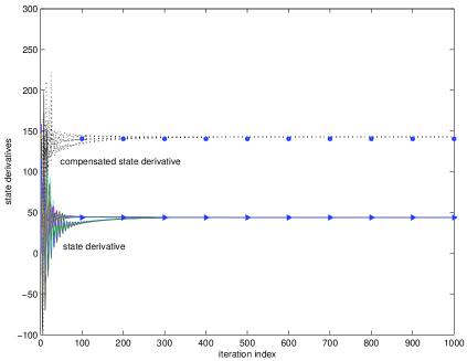
Figure 2: Uncompensated running estimate (solid lines), i.e. $\dot{{x}}_{i}(t;\mbox{\boldmath$y$})$ and compensated running estimate (dotted lines), i.e. $\dot{{x}}_{i}(t;\mbox{\boldmath$y$})/\dot{{x}}_{i}(t;\mbox{\boldmath$1$})$.

In summary, in this work we have derived the conditions allowing a distributed consensus mechanism to reach globally optimal decision statistics, in the presence of multipath propagation in the link between each pair of nodes. The method is valid for real (baseband) channels and it requires that the summation of the channel coefficients over each link is strictly positive. Thanks to the closed form expression derived in this paper, we have also shown how to get unbiased, globally optimal estimates, without the need to resolve the signals received from different nodes (thus allowing for a very simple MAC mechanism), nor to estimate the channel coefficients. A crucial investigation, motivated from this work, is the design of the most appropriate radio interface allowing for the internode interaction enabling the distributed consensus.

5 Appendix

Part of the proof of the theorem is based on the same approach we followed in [11, Appendix C]. Thus, in the following we make use of the general results of [11, Appendix C] and we focus only on the specific aspects of the model used in this paper. We start studying the existence of a synchronized state in the form (4). Then, we prove that such a state is also globally asymptotically stable (cf. Definition 1). Throughout the proof, we assume that conditions a1)-a4) are satisfied and that the digraph ${\mathscr{G}}$ associated to (2) is QSC. In the following, for the sake of notation simplicity, we drop the dependence of the state function from the observation, as this dependence does not play any role in our proof.

Existence of a synchronized state: The set of delayed differential equations (2) admits a solution in the form

$$x_{i}^{\star}(t)={\alpha}t+x_{i,0}^{\star},\,\quad i=1,\ldots,N,\vspace{-0.1cm}$$ (5)

where ${\alpha\in\mathbb{R}}$ and $\{x_{i,0}^{\star}\}$ are a set of coefficients that depend in general on the system parameters and on the initial conditions, if and only if $\{x_{i}^{\star}(t)\}$ satisfies (2), i.e., if and only if there exist $\alpha$ and $\{x_{i,0}^{\star}\}$ such that the following system of linear equations is feasible:

$$\frac{c_{i}\Delta_{i}(\alpha)}{K}+\sum\nolimits_{j\in\mathcal{N}_{i}}\left(\sum\nolimits_{l=1}^{L}a_{ij}^{(l)}\right)\left(x_{j,0}^{\star}-x_{i,0}^{\star}\right)=0,\vspace{-0.2cm}$$ (6)

$\forall i=1,\ldots,N,$ where

$$\Delta_{i}(\alpha)\triangleq g_{i}(y_{i})-\alpha\left(1+\frac{K}{c_{i}}\sum\nolimits_{j\in\mathcal{N}_{i}}\sum\nolimits_{l=1}^{L}a_{ij}^{(l)}\,\tau_{ij}^{(l)}\right).$$ (7)

Introducing the weighted Laplacian $\mathbf{L}=\mathbf{L}({\mathscr{G}})$ associated to ${\mathscr{G}}$, system (6) can be equivalently rewritten in vector form as

$$K\mathbf{Lx}_{0}^{\star}=\mathbf{D}_{\mathbf{c}}\boldsymbol{\Delta}\,(\alpha),\vspace{-0.1cm}$$ (8)

where $\mathbf{x}_{0}^{\star}\triangleq[x_{1,0}^{\star},\ldots,x_{N,0}^{\star}]^{T},$ $\mathbf{D}_{\mathbf{c}}\triangleq\mathop{\mathrm{d}iag}(c_{1},\ldots,c_{N}),$ and $\boldsymbol{\Delta}\,(\alpha)$ $\triangleq[\Delta_{1}(\alpha),\ldots,\Delta_{N}(\alpha)]^{T},$ with $\Delta_{i}(\alpha)$ defined in (7). Observe that, because of a2) and the quasi-strong connectivity of ${\mathscr{G}}$, the graph Laplacian $\mathbf{L}$ has the following properties: i) $\mathrm{rank}(\mathbf{L})=N-1;$ ii) $\mathcal{N}(\mathbf{L})=\mathcal{R}\left(\mathbf{1}_{N}\right);$ and iii) $\mathcal{N}(\mathbf{L}^{T})=\mathcal{R}\left(\mathbf{\gamma}\right),$ where $\mathcal{N}(\cdot)$ and $\mathcal{R}(\cdot)$ denote the (right) null-space and the range space operators, respectively, and $\mathbf{\gamma}$ is a left eigenvector of $\mathbf{L}$ corresponding to the (simple) zero eigenvalue of $\mathbf{L}$, i.e., $\mathbf{\gamma}^{T}\mathbf{L}=\mathbf{0}^{T}$. It follows from i)-iii) that, for any given $\alpha,$ (8) admits a solution if and only if $\ \mathbf{D}_{\mathbf{c}}\boldsymbol{\Delta}\,(\alpha)\in\mathcal{R}\left(\mathbf{L}\right)$. Using again properties i)-iii), we have: $\mathbf{D}_{\mathbf{c}}\boldsymbol{\Delta}(\alpha)\in\mathcal{R}\left(\mathbf{L}\right)\Leftrightarrow\mathbf{\gamma}^{T}\mathbf{D}_{\mathbf{c}}\boldsymbol{\Delta}(\alpha)=0.$ It is easy to check that the value of $\alpha$ that satisfies the latter condition is $\alpha=\alpha^{\star},$ with $\alpha^{\star}$ defined in (4). Hence, if $\alpha=\alpha^{\star},$ the synchronized state in the desired form (5) is a solution to (2), for any given set of $\{\tau_{ij}^{(l)}\},$ $\{g_{i}\},$ $\{c_{i}\}$, $\{a_{ij}^{(l)}\}$ and $K>0$.

The structure of the left eigenvector $\mathbf{\gamma}$ associated to the zero eigenvalue of $\mathbf{L}$ as given in the theorem follows from  [11, Lemma 4].

Setting $\alpha=\alpha^{\star}$, system (8) admits $\infty^{1}$ solutions, given by $\mathbf{x}_{0}^{\star}=\frac{1}{K}\mathbf{\mathbf{L}^{\sharp}D}_{\mathbf{c}}\boldsymbol{\Delta}(\alpha^{\star})+\mathcal{R}\left(\mathbf{1}_{N}\right)\triangleq\overline{\mathbf{x}}_{0}+\mathcal{R}\left(\mathbf{1}_{N}\right),$ where

$$\overline{\mathbf{x}}_{0}\triangleq\mathbf{\mathbf{L}^{\sharp}D}_{\mathbf{c}}\boldsymbol{\Delta}(\alpha^{\star})/K,\vspace{-0.1cm}$$ (9)

$\Delta_{i}(\alpha^{\star})$ is obtained by (7) setting $\alpha=\alpha^{\star}$ and $\mathbf{\mathbf{L}}^{\sharp}$ is the generalized inverse of the Laplacian $\mathbf{\mathbf{L}}$.

Global asymptotic stability: We prove now that the synchronized state of system (2) is globally asymptotically stable. To this end, we use the following intermediate results.

Let $\mathbf{\mathbb{C}}_{+}=\{s\in\mathbf{\mathbb{C}}:\mathop{\mathrm{R}e}\{s\}>0\},$ $\mathbf{\mathbb{C}}_{-}=\{s\in\mathbf{\mathbb{C}}:\mathop{\mathrm{R}e}\{s\}<0\},$ and $\overline{\mathbf{\mathbb{C}}}_{+}$ be the closure of $\mathbf{\mathbb{C}}_{+}$, i.e., $\overline{\mathbf{\mathbb{C}}}_{+}=\{s\in\mathbf{\mathbb{C}}:\mathop{\mathrm{R}e}\{s\}\geq 0\}.$ Denoting by $\mathcal{H}^{n\times m}$ the set of $n\times m$ matrices whose entries are analytic and bounded functions in $\mathbf{\mathbb{C}}_{+},$ let us introduce the degree matrix $\boldsymbol{\Delta}\geq\mathbf{0}$ (where “$\geq$”has to be intended component-wise) and the complex matrix $\mathbf{H}(s)\in\mathbf{\mathbb{C}}^{N\times N}\mathbf{,}$ defined respectively as

$$\boldsymbol{\Delta}\triangleq\mathop{\mathrm{d}iag}\left(k_{1}\deg\nolimits_{\text{in}}(v_{1}),...,k_{N}\deg\nolimits_{\text{in}}(v_{N})\right),\qquad\left[\mathbf{H}(s)\right]_{ij}\triangleq\left\{\begin{array}[]{ll}0,&\text{if }i=j,\\ k_{i}\sum\nolimits_{l=1}^{L}a_{ij}^{(l)}e^{-s\tau_{ij}^{(l)}},&\text{if }i\neq j,\end{array}\right.\vspace{-0.2cm}$$ (10)

where $\deg\nolimits_{\text{in}}(v_{i})=$ $\sum_{j\in\mathcal{N}_{i}}\sum\nolimits_{l=1}^{L}a_{ij}^{(l)}\geq 0$ is the in-degree of node $v_{i}$ and $k_{i}\triangleq K/c_{i}>0.$ Observe that $\mathbf{H}(s)\in\mathcal{H}^{N\times N}\mathbf{.}$

Lemma 1

Consider the following linear functional differential equation:

$$\begin{array}[]{l}\dot{{x}}_{i}(t)=k_{i}\mathop{\displaystyle\sum}\nolimits_{j\in\mathcal{N}_{i}}\mathop{\displaystyle\sum}\nolimits_{l=1}^{L}a_{ij}^{(l)}\left(x_{j}(t-\tau_{ij}^{(l)})-x_{i}(t)\right),\quad\,\,t>0,\\ x_{i}(\vartheta)=\phi_{i}(\vartheta),\quad\vartheta\in[-\tau,\ 0].\end{array}\quad\begin{array}[]{l}i=1,\ldots,N,\end{array}$$ (11)

and assume that the following conditions are satisfied:

1. The initial value functions $\mathbf{\phi}$ are taken in the set $\ \mathcal{C}^{1}$ of continuously differentiable functions that are bounded in the norm $\left|\mathbf{\phi}\right|_{s}=\sup_{-\tau\leq\vartheta\leq 0}\left\|\mathbf{\phi}(\vartheta)\right\|_{\infty},\$and the solutions $\mathbf{x}(t)$ with initial functions $\mathbf{\phi}$ are bounded;

2. The characteristic equation associated to (11)

   $$p(s)\triangleq\det\left(s\mathbf{I}+\boldsymbol{\Delta}-\mathbf{H}(s)\right)=0,$$ (12)

   with $\boldsymbol{\Delta}$ and $\mathbf{H}(s)$ defined in (10), has all roots $\{s_{r}\}_{r}\in$ $\mathbf{\mathbb{C}}_{-},$ with  at most one simple root at $s=0.$

Then, system (11) is marginally stable, i.e., $\forall\mathbf{\phi}\in\mathcal{C}^{1}$ and  $\mathop{\mathrm{R}e}\{s_{1}\}<c<0,$ there exist $t_{1}$ and $\alpha,$ with $t_{0}<t_{1}<+\infty$ and $0<\alpha<+\infty,$ independent of $\mathbf{\phi,}$ and a vector $\mathbf{x}^{\infty},$ with $\left\|\mathbf{x}^{\infty}\right\|<+\infty,$ such that

$$\left\|\mathbf{x}(t)-\mathbf{x}^{\infty}\right\|\leq\alpha\left|\mathbf{\phi}\right|_{s}e^{ct},\qquad\forall t>t_{1}.$$ (13)

Proof. Because of space limitation, we omit the proof that can be obtained following the same steps of the proof in [11, Lemma 5], after observing that system (11) can be rewritten in the canonical form of [16, Ch. 6, Eq. (6.3.2)], [17, Ch. 3, Eq. (3.1)].  

Lemma 2 ([15, Theorem 2.2])

Let $\mathbf{H}(s)\in\mathcal{H}^{N\times N}$ and $\rho\left(\mathbf{H}(s)\right)$ denote the spectral radius of $\mathbf{H(}s\mathbf{).}$ Then, $\rho\left(\mathbf{H}(s)\right)$ is a subharmonic bounded (above) function on $\overline{\mathbf{\mathbb{C}}}_{+}$. $\square$

We are ready to prove the global asymptotic stability of the synchronized state of (2). Applying the following change of variables: $\Psi_{i}(t)\triangleq x_{i}(t)-\left(\alpha^{\star}t+\overline{x}_{i,0}\right)$, for all $i=1,\ldots,N,$ where $\alpha^{\star}$ and $\{\overline{x}_{i,0}\}$ are defined in (4) and (9), respectively, and using (9), the original system (2) can be equivalently rewritten in terms of $\{\Psi_{i}(t)\}_{i}$ as

$$\dot{\Psi}_{i}(t)=k_{i}\mathop{\displaystyle\sum}\nolimits_{j\in\mathcal{N}_{i}}\mathop{\displaystyle\sum}\nolimits_{l=1}^{L}a_{ij}^{(l)}\left(\Psi_{j}(t-\tau_{ij}^{(l)})-\Psi_{i}(t)\right),\text{ \ \ }t\geq 0,$$ (14)

with $\Psi_{i}(\vartheta)=\phi_{i}(\vartheta)\triangleq\widetilde{\phi}_{i}(\vartheta)-\alpha^{\star}\vartheta-\overline{x}_{i,0}$ for $\vartheta\in[-\tau,\ 0],$ where $\{\widetilde{\phi_{i}}\}$ are the initial value functions of the original system (2).

It follows from (14) that the synchronized state of system (2), as given in (5) (with $\alpha=\alpha^{\star}$), is globally asymptotically stable (according to Definition 1) if system (14) is marginally stable. According to Lemma 1, the marginal stability of system (14) is guaranteed if: b1) the trajectories $\{\Psi_{i}(t)\}$ are bounded for all $t>0,$ given $\mathbf{\phi}\in\mathcal{C}^{1};$ b2) the characteristic equation (12) associated to (14), has all roots in $\mathbf{\mathbb{C}}_{-},$ with  at most one simple root at $s=0.$

Following the same steps as in [11, Appendix C], one can prove that, under a1)-a3), all the solutions $\{\Psi_{i}(t)\}$ to (14), with initial conditions in $\mathcal{C}^{1},$ are uniformly bounded, as required by assumption b1) in Lemma 1. Because of space limitation we omit the details. We study instead the characteristic equation (12), and prove that, under a1)-a3) and the quasi-strong connectivity of the digraph, assumption b2) of Lemma 1 is satisfied.

First of all, observe that, since $\boldsymbol{\Delta}-\mathbf{H}(0)=K\mathbf{D}_{c}\mathbf{L}$, we have

$$p(0)=\det\left(\boldsymbol{\Delta}-\mathbf{H}(0)\right)=\det\left(K\mathbf{D}_{c}\right)\det\left(\mathbf{L}\right)=0,$$ (15)

where the last equality in (15) is due to $\mathrm{rank}(\mathbf{L})=N-1$. It follows from (15) that $p(s)$ has a root in $s=0,$ corresponding to the zero eigenvalue of the Laplacian $\mathbf{L}$ (recall that $\det\left(K\mathbf{D}_{c}\right)\neq 0$). Since the digraph is assumed to be QSC, according to [11, Corollary 2], such a root is simple. Thus, to complete the proof, we need to show that $p(s)$ does not have any solution in $\overline{\mathbf{\mathbb{C}}}_{+}\backslash\{0\},$ i.e.,

$$\det\left(s\mathbf{I+}\boldsymbol{\Delta}-\mathbf{H}(s)\right)\neq 0,\quad\forall s\in\overline{\mathbf{\mathbb{C}}}_{+}\backslash\{0\}.$$ (16)

Since $s\mathbf{I+}\boldsymbol{\Delta}$ is nonsingular in $\overline{\mathbf{\mathbb{C}}}_{+}\backslash\{0\}$ [recall that, under a1)-a2), $\boldsymbol{\Delta}\geq\mathbf{0}$, with at least one positive diagonal entry], (16) is equivalent to

$$\det\left(\mathbf{I-}\left(s\mathbf{I+}\boldsymbol{\Delta}\right)^{-1}\mathbf{H}(s)\right)\neq 0,\quad\forall s\in\overline{\mathbf{\mathbb{C}}}_{+}\backslash\{0\},$$ (17)

which leads to the following sufficient condition for (16):

$$\rho\left(s\right)\triangleq\rho\left(\left(s\mathbf{I+}\boldsymbol{\Delta}\right)^{-1}\mathbf{H}(s)\right)<1,\quad\forall s\in\overline{\mathbf{\mathbb{C}}}_{+}\backslash\{0\}.$$ (18)

Since $\left(s\mathbf{I+}\boldsymbol{\Delta}\right)^{-1}\in\mathcal{H}^{N\times N}$ and $\mathbf{H}(s)\in\mathcal{H}^{N\times N}$, it follows from Lemma 2 that the spectral radius $\rho\left(s\right)$ in (18) is a subharmonic function on $\overline{\mathbf{\mathbb{C}}}_{+}.$ As a direct consequence, we have, among all, that $\rho\left(s\right)$ is a continuous bounded function on $\overline{\mathbf{\mathbb{C}}}_{+}$ and satisfies the maximum modulus principle (see, e.g., [15] and references therein): $\rho\left(s\right)$ achieves its global maximum only on the boundary of $\overline{\mathbf{\mathbb{C}}}_{+}.$ Since $\rho\left(s\right)$ is strictly proper in $\overline{\mathbf{\mathbb{C}}}_{+},$ i.e., $\rho\left(s\right)\rightarrow 0$ as $\left|s\right|\rightarrow+\infty$ while keeping $s\in\overline{\mathbf{\mathbb{C}}}_{+}$, it follows that $\sup_{s\in\mathbf{\mathbb{C}}_{+}}\rho\left(s\right)<\sup_{\omega\in\mathbb{R}}\rho\left(j\omega\right).$ According to the latter inequality, condition (18) is satisfied if

$$\rho\left(j\omega\right)=\rho\left(\left(j\omega\mathbf{I+}\boldsymbol{\Delta}\right)^{-1}\mathbf{H}(j\omega)\right)<1,\quad\forall\omega\in\mathbb{R}\backslash\{0\}.$$ (19)

Denoting by $\left\|\mathbf{A}\right\|_{\infty}\triangleq\max_{r}\sum\nolimits_{q}|\left[\mathbf{A}\right]_{rq}|$ the maximum row sum matrix norm and using $\rho\left(\mathbf{A}\right)\leq\left\|\mathbf{A}\right\|_{\infty}$ $\forall\mathbf{A\in\mathbb{C}}^{N\times M}$ [18], we have

$$\rho\left(j\omega\right) \leq \left\|\left(j\omega\mathbf{I+}\boldsymbol{\Delta}\right)^{-1}\mathbf{H}(j\omega)\right\|_{\infty}\!\!=\!\max_{r}\frac{\mathop{\textstyle\sum}\nolimits_{q\in\mathcal{N}_{r}}\left|k_{r}H_{rq}(j\omega)\right|}{\left|j\omega+k_{r}\mathop{\textstyle\sum}\nolimits_{q\in\mathcal{N}_{r}}H_{rq}(0)\right|}\leq\max_{r}\frac{\mathop{\textstyle\sum}\nolimits_{q\in\mathcal{N}_{r}}\left|H_{rq}(j\omega)\right|}{\mathop{\textstyle\sum}\nolimits_{q\in\mathcal{N}_{r}}H_{rq}(0)}\leq 1,$$

where in the last inequality we used (3) [see assumption a2)]. Since in the second inequality, the equality is reached if and only if $\omega=0,$ we have $\rho\left(j\omega\right)<1$ for all $\omega\neq 0,$ which guarantees that condition (18) is satisfied. Hence, according to Lemma 1, given any set of initial conditions $\{\phi_{i}\}$ satisfying a4), the trajectories $\mathbf{\Psi}(t)\rightarrow\mathbf{\Psi}^{\infty}$ as $t\rightarrow+\infty,$ with exponential rate arbitrarily close to $r\triangleq-\{\min_{i}|\mathop{\mathrm{R}e}\{s_{i}\}|:p(s_{i})=0\,\,\text{and}\,\,s_{i}\neq 0\}$, where $p(s)$ is defined in (12) and $\mathbf{\Psi}^{\infty}\in\mathcal{R}(\mathbf{1}_{N})$ (because of $\mathbf{L\Psi}^{\infty}=\mathbf{0}$ and $\mathrm{rank}(\mathbf{L})=N-1$). In other words, system (14) exponentially reaches the consensus on the state.

Necessity: The necessity of quasi-strong connectivity of the digraph for the network to reach a global consensus can be proved as in [11, Appendix C.2] by showing that, if the digraph associated to (2) is not QSC, different clusters of nodes synchronize on different values [11, Corollary 1]. This local synchronization is in contrast with the definition of (global) synchronization, as given in Definition 1. Hence, if the overall network has to synchronize, the digraph associated to the system must be QSC.

References

- [1] R. Olfati-Saber, J. A. Fax, R. M. Murray, “Consensus and Cooperation in Networked Multi-agent Systems,” in Proc. of the IEEE, vol. 95, no. 1, pp. 215-233, Jan. 2007.
- [2] W. Ren, R. W. Beard, and E. M. Atkins, “Information Consensus in Multivehicle Cooperative Control: Collective Group Behavior Through Local Interaction,” IEEE Control Systems Mag., vol. 27, no. 2, pp. 71-82, April 2007.
- [3] R. Olfati-Saber and R.M. Murray, “Consensus Problems in Networks of Agents with Switching Topology and Time-Delays,” IEEE Trans. on Automatic Control, vol. 49, pp. 1520-1533, Sep., 2004.
- [4] M.G. Earl, and S.H. Strogatz, “Synchronization in Oscillator Networks with Delayed Coupling: A Stability Criterion,”Physical Rev. E, Vol. 67, pp. 1-4, 2003.
- [5] A. Papachristodoulou and A. Jadbabaie, “Synchronization in Oscillator Networks: Switching Topologies and Presence of Nonhomogeneous delays,”in Proc of the IEEE ECC-CDC ’05, Dec. 2005.
- [6] D.J. Lee and M.W. Spong, “Agreement With Non-uniform Information Delays,” in Proc. of the ACC ’06, June 2006.
- [7] J. N. Tsitsiklis, D. P. Bertsekas, M. Athans, “Distributed Asynchronous Deterministic and Stochastic Gradient Optimization Algorithms,” IEEE Trans. on Automatic Control, pp. 803–812, Sep. 1986.
- [8] D. P Bertsekas and J.N. Tsitsiklis, Parallel and Distributed Computation: Numerical Methods, Athena Scientific, 1989.
- [9] V. D. Blondel, J. M. Hendrickx, A. Olshevsky, and J. N. Tsitsiklis, “Convergence in Multiagent Coordination, Consensus, and Flocking,” in Proc. of the IEEE CDC-ECC’05, Dec. 2005.
- [10] S. Boyd, A. Ghosh, B. Prabhakar, D. Shah, “Randomized gossip algorithms,”in IEEE Trans. on Information Theory, Vol. 52, pp. 2508–2530, June 2006.
- [11] G. Scutari, S. Barbarossa, and L. Pescosolido, “Distributed Decision Through Self-Synchronizing Sensor Networks in the Presence of Propagation Delays and Asymmetric Channels,” in IEEE Trans. on Sign. Proc., vol. 56, no. 4, pp.1667–1684, April 2008.
- [12] S. Barbarossa, and G. Scutari, “Decentralized Maximum Likelihood Estimation for Sensor Networks Composed of Self-synchronizing Locally Coupled Oscillators,”, IEEE Trans. on Sign. Proc., vol. 55, no. 7, pp. 3456–3470, July 2007.
- [13] S. Barbarossa and G. Scutari, “Bio-inspired Sensor Network Design: Distributed Decision Through Self-synchronization,” IEEE Sign. Proc. Magazine, vol. 24, no. 3, pp. 26–35, May 2007.
- [14] W. Rudin, Real and Complex Analysis, McGraw-Hill, International Student Ed., 1970.
- [15] S. Boyd and S. A. Desoer, “Subharmonic Functions and Performance Bounds on Linear Time-Invariant Feedback Systems,”in IMA Jour. of Math. Control Inf., Vol. 2, pp. 153-170, 1985.
- [16] R. Bellman and K.L. Cooke, Differential-Difference Equations, New York Academic Press, 1963.
- [17] K. Gu, V.L. Kharitonov, J. Chen, Stability of Tyme-Delay Systems, Control Engineering Series, Birkhauser, 2002.
- [18] R. A. Horn and C. R. Johnson, Matrix Analysis, Cambridge Univ. Press, 1985.
- [19] G. Mergen, L. Tong, “Type-based Estimation over Multiaccess Channels,”in IEEE Trans. on Signal Proc., Vol. 54, pp. 613–626, Febr. 2006.
- [20] L. Pescosolido and S. Barbarossa “Distributed Decision in Sensor Networks based on Local Coupling through Pulse Position Modulated Signals,”in Proc. of IEEE ICASSP 2008, March 30 - April 4, 2008, Las Vegas, NV, (USA).
- [21] L. Pescosolido, S. Barbarossa, and G. Scutari, “Radar Sensor Networks with Distributed Detection Capabilities,”in Proc. of IEEE Radar Conference 2008, Sheraton Golf Parco dei Medici, May 26-30, 2008, Rome, Italy.
- [22] S. Barbarossa, G. Scutari, A. Swami, “Achieving Consensus in Self-Organizing Wireless Sensor Networks: The Impact of Network Topology on Energy Consumption,” in Proc. of IEEE ICASSP 2007, April 15-20, Honolulu, Hawaii (USA).