Bohmian approach to spin-dependent time of arrival for particles in a uniform field and for particles passing through a barrier
Abstract
It is known that Lorentz covariance fixes uniquely the current and the associated guidance law in the trajectory interpretation of quantum mechanics for spin- particles. In the nonrelativistic domain this implies a guidance law for electrons which differs by an additional spin-dependent term from the one originally proposed by de Broglie and Bohm. Although the additional term in the guidance equation may not be detectable in the quantum measurements derived solely from the probability density , it plays a role in the case of arrival-time measurements. In this paper we compute the arrival time distribution and the mean arrival time at a given location, with and without the spin contribution, for two problems: 1) a symmetrical Gaussian packet in a uniform field and 2) a symmetrical Gaussian packet passing through a 1D barrier. Using the Runge-Kutta method for integration of the guidance law, Bohmian paths of these problems are also computed.
pacs:
03.65.Ta, 03.75.-bKeywords: Spin, Nonrelativistic limit, Modified guidance law, Bohmian mechanics, Arrival time
I introduction
In classical mechanics, each particle follows a definite trajectory, and so it is clear what is meant by the time at which a particle arrives at a given place. In quantum mechanics, as opposed to classical physics, the meaning of the arrival time of a particle at a given location is not evident when the finite extent of the wave function and its spreading becomes relevant. Moreover, in the quantum case one expects an arrival time distribution, and there are different proposals for this (see e.g. the review article in MuLe-PhysRep-2000 , and the book MuSaEg-book-2002 .) As pointed out by Hannstein et al HaHeMu-JPB-2005 , these arrival time distributions have been controversial, since they are derived from purely theoretical arguments without specifying a measurement procedure. The lack of a self-adjoint arrival-time operator conjugate to the free Hamiltonian lies at the core of the difficulties in the formulation of quantum arrival times HeSeMu-PRA-2003 . In Bohm’s interpretation of nonrelativistic quantum mechanics BoI-PR-1952 ; BoII-PR-1952 ; HiBo-book-1993 ; Ho-book-1993 ; DuGoZa-1992-JSP ; DuGoZa-1996-book ; Tu-2004-AJP , an electron is a particle that has a well defined trajectory and so the definition of arrival-time distributions is unambiguous. In Bohm’s trajectory approach to the calculation of various characteristic times, it is only the particle component of the particle that is being clocked. If the arrival-time detector is not included in the Hamiltonian, then one has an expression for the ideal or intrinsic arrival-time distribution MuSaEg-Le-book-2002 . The arrival-time problem is unambiguously solved in the Bohmian mechanics, where for an arbitrary scattering potential , one finds Le-PhyslettA-1993 ; MuSaEg-Le-book-2002 ; Le-book-1996 ; Le-PRA-1998 for those particles that actually reach ; the arrival-time distribution being given by the modulus of the probability current density, i.e., . In nonrelativistic quantum mechanics, the form of the current density is not uniquely determined by the continuity equation, a point which has been mentioned by a number of authors DeGh-Found.phys-1998 ; Ho-Found.phys-1998 ; Fi-PRA-1999 . It is determined only up to a divergenceless vector. For instance, one can construct a new current by adding the divergenceless current to the current . The newly defined current also satisfies the continuity equation, with the same probability density. Although the additional contribution in the guidance equation may not be detectable in quantum measurements derived solely from the probability density , it plays a role in the case of arrival-time measurements. In the case of spin- particles, Holland Ho-PRA-1999 showed that the particle current in the relativistic spin- Dirac theory is unique. Demanding that the non-relativistic spin- particle current be obtained from the nonrelativistic limit of the Dirac current, this nonrelativistic current is also unique. Struyve et al StBaNeWe-PLA-2004 have considered the uniqueness of paths for spin- and spin- particles. The spin-dependent Bohm trajectories have been investigated for hydrogen eigenstates CoVr-PLA-2002 and an electronic transition in hydrogen CoVr-JPA-2003 .
It was argued that for free spin eigenstates, spin contributions would in principle be experimentally distinguishable for arrival-time distributions of spinless and spin- particles AlMaDiSh-PRA-2003 . Holland et al HoPh-PRA-2003 have explored some of the implications of the modified guidance law in the case of the two-slit quantum interference. In this case, the trajectories cross each other and they also cross the symmetry axis.
The aim of the present paper is to explore some of the implications of the revised nonrelativistic guidance equation. Sec. II contains a very brief review of relevant parts of Bohm’s interpretation of quantum mechanics. In Sec. III, by using the nonrelativistic limit of the Dirac current density, numerical computations of the effect of the spin-dependent term on arrival time at a given location, are presented for both a Gaussian wave in a uniform field and a Gaussian wave passing through a barrier.
II Bohm’s trajectory interpretation of quantum mechanics and the arrival time distributions
In nonrelativistic Bohmian mechanics the world is described by point-like particles which follow trajectories determined by a law of motion. The evolution of the positions of these particles are guided by a wave function which itself evolves according to the Schrödinger equation. Bohmian mechanics makes the same predictions as the ordinary nonrelativistic quantum mechanics for the results of any experiment, provided we assume a random distribution for configuration of the system and the apparatus at the beginning of the experiment, given by . If the probability density for the configuration satisfies at some initial time , then the density to which this is carried by the continuity equation at any time is also given by Bo-PR-1953 . As most of the quantum measurements boil down to position measurements, Bohm’s theory and the standard quantum mechanics generally yield the same detection probabilities. The situation is different, however, if one considers, for example, measurements involving time-related quantities, such as arrival times, tunnelling times, etc. Bohm’s theory makes unambiguous predictions for such measurements, but there is no consensus about what these quantities should be in the conventional quantum mechanics St-quant-2005 . Given the initial position of a particle with the initial wave function , its subsequent trajectory is uniquely determined by the simultaneous integration of the time dependent Schrödinger equation, and the guidance equation , in which . For spinless particles, the Schrödinger equation yields:
| (1) |
But, for systems with more than one spatial dimension the probability current density, and hence the particle equation of motion, is not uniquely defined within nonrelativistic quantum mechanics. But, Holland Ho-PRA-1999 has shown that the probability current density deduced from the continuity equation is uniquely defined for Dirac electrons, when Lorentz covariance is imposed. Taking the nonrelativistic limit for a spin eigenstate in the absence of a magnetic field, one gets
| (2) | |||||
where
| (3) |
is the spin vector associated with the spin eigenstate , which is a two-component spinor normalized to unity (). The nonrelativistic particle is, in effect, guided by the two-component wave function , and the original expression for the nonrelativistic velocity field should then be replaced by
| (4) |
A striking property of the spin-dependent term is that the components of the particle motion in orthogonal directions are generally mutually dependent, even when the wave function factorizes in these direction. For a 3D system with a wave function which is in the factorized form at , we have
at , and for , Eq. (4) becomes
| (5) |
where we have used the notation and so on. For a nonrelativistic guiding wave of the form , with being a solution of the Schrödinger equation and being a fixed spinor, Bohm’s trajectory result for the distribution of particle arrival times , at a given location , is given by MuSaEg-Le-book-2002
| (6) |
The mean arrival time of the particles reaching a detector located at is given by
| (7) |
in the presence of the spin-dependent contribution and
| (8) |
in the absence of the spin-dependent contribution. It must be mentioned that the definition of the mean arrival time used in Eq. (8) is not a uniquely derivable result within standard quantum mechanics. We compute the arrival time distribution and the mean arrival time at a given location for two problems: 1) a symmetrical Gaussian packet in a uniform field and 2) a symmetrical Gaussian packet passing through a 1D barrier with and without the spin contribution. Using the Runge-Kutta method for the integration of the guidance law, Bohmian paths of these problems, have been also computed.
II.1 Symmetric Gaussian packet in a uniform field
For the potential , the wave function and the probability density at time , calculated from Ho-book-1993 , are given by:
| (9) |
provided that this symmetrical Gaussian wave function is centred around the origin at . In the Eq. (II.1), , and is the group velocity. The Eq. (II.1) is in the factorized form in three coordinate directions. We choose the uniform field and the group velocity to be in the direction i.e., and and the spin vector in the direction. The speed of the wave packet’s centre in the and directions has been set equal to zero and therefore this function will spread but will not propagate in these directions. Using the Eq. (II), one gets for this factorized wave
| (10) |
from which one can compute Bohmian trajectories. In the direction, one gets , in which is the -component of the initial position of the particle.
II.2 Symmetric Gaussian packet passing through a barrier in the x-direction
suppose for and zero otherwise. The wave function at time is given by
| (11) |
in which
| (12) |
where is the group velocity and
| (13) |
is the transmission probability with . Again, the speed of the wave packet’s centre in and directions has been set equal to zero and therefore this function will spread but not propagate in these directions. For the motion in the direction, one gets
| (14) |
in which is the -component of the initial position of the particle.
III Numerical Results
Numerical calculations are presented for a case of symmetric Gaussian packet in a uniform field and a case of symmetric Gaussian packet passing through a barrier in the x-direction. We compute the mean arrival time and the arrival time distribution with and without the spin-dependent term. Using the Runge-Kutta method for the integration of guidance equation, we compute some Bohmian paths for each case.
III.1 Symmetric Gaussian packet in a uniform field
The initial wave packet is peaked at , with Å. The detector position is chosen at Å.
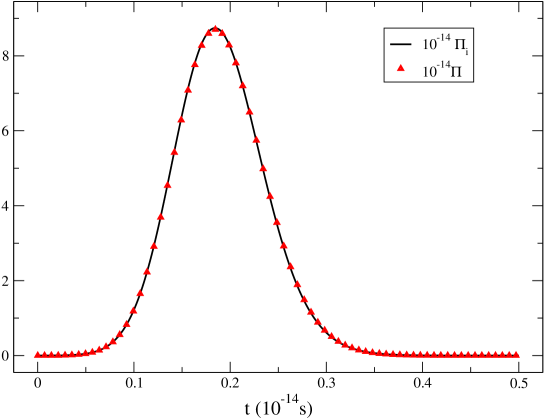
Fig. 1 shows the arrival time distribution of electrons for , corresponding to particles in a gravity field, with ev and .
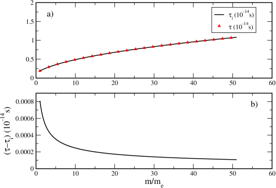
Fig. 2 shows the mean arrival time versus the mass of the arriving particle for a fixed value of (ev). From this figure, it follows that the spin-dependent term increases the mean arrival time () and has very small effect on the mean arrival time at the given location, and the quantity is decreased with mass.
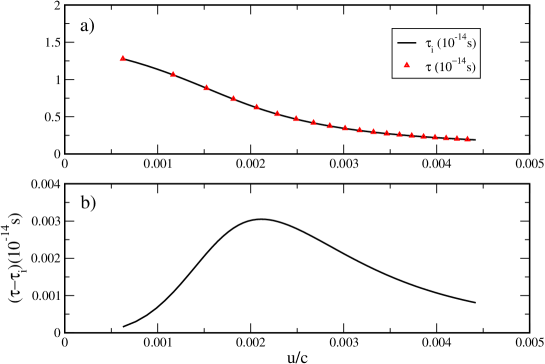
Fig. 3 shows the mean arrival time of electrons versus the ratio of the group velocity to the light velocity (Note that we have fixed the mass). It follows from this figure that the spin-dependent term increases the arrival time () and has very small effect on the mean arrival time at the given location and that the quantity is increased with the initial group velocity at first and then is decreased with it.
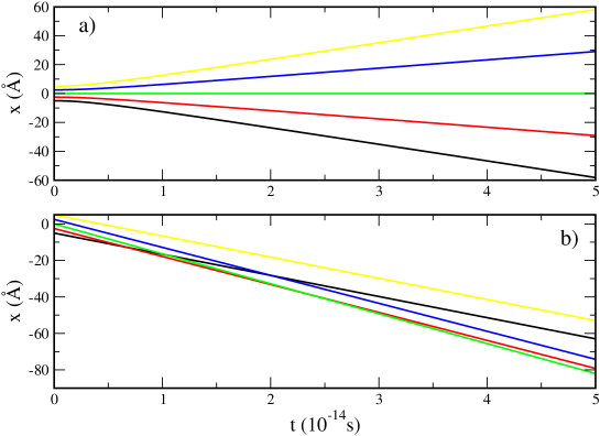
Fig. 4 shows some Bohmian paths for electrons. One can see that some trajectories cross each other when one considers the spin-dependent term. It should be noted that trajectories cross each other for different values of the coordinate. Consequently there is no problem with the single-valuedness of the wave function. The spin-dependent term can also change the fate of the individual trajectories. There are some trajectories that don’t reach the detector location, with the spin-dependent term, but reach the detector location without this term.
III.2 Symmetric Gaussian packet passing through a barrier in the x-direction
The initial wave packet is peaked at with Å. The detector location is chosen at Å.
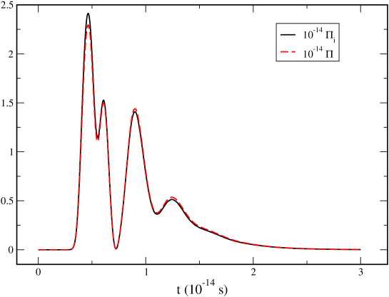
Fig. 5 shows the arrival time distribution of electrons, for ev, ev and Å.
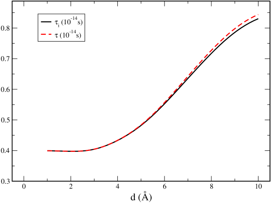
Fig. 6 shows the mean arrival time of electrons at the given location, versus width of the barrier. From this figure, it follows that the spin-dependent term increases the mean arrival time () and the quantity is increased with the width of the barrier.
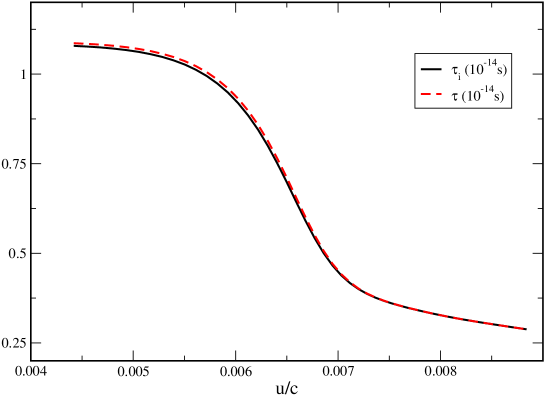
Fig. 7 shows the mean arrival time of electrons versus the ratio of the group velocity to the light velocity for Å. It follows from this figure that the spin-dependent term increases the arrival time () and has very small effect on the mean arrival time at the specified location, and that the quantity is decreased with the initial group velocity. Note that we could not decrease the initial energy (or the initial group velocity) as we want,as in the Fig. 3, because if , then the transmission probability would be very small and no particle can cross the barrier to reach the detector position.
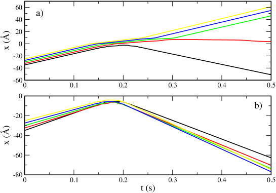
Fig. 8 shows some Bohmian paths for electrons. One can see that trajectories cross each other (Fig. 8), when one considers the spin-dependent term. As the Fig. 4 they cross each other for different values of the coordinate. The spin-dependent term can also change the fate of the individual trajectories. There are some trajectories that don’t reach the barrier, with the spin-dependent term, but they cross the barrier without this term. However, ensemble averaging yields the same transmission and reflection probabilities. The spin-dependent term plays a role only in time related measurements.
IV Summary and discussion
Spin has a very small effect on the mean arrival time at a given location in the nonrelativistic domain, but it has a significant effect on the fate of individual Bohmian paths. Bohmian paths can cross each other, when one considers the spin-dependent term. The quantity changes with the mass of the arriving particle, with the group velocity of the wave packet and also with the width of the barrier, but, the difference is very small.
V Acknowledgment
We are very indebted to H. Nikolic for helpful discussions and corrections and valuable suggestions. S. V. M. is grateful to J. G. Muga and A. del Campo for providnig useful information.
References
- (1) J. G. Muga and C. R. Leavens, Phys. Rep 338 (2000) 353
- (2) J. G. Muga, R. Sala and I. L. Egusquiza(eds), Time in Quantum Mechanics (Berlin: Springer (2002))
- (3) V. Hannstein, G. C. Hegerfeldt and J. G. Muga, J .Phys. B: Mol. Opt. Phys. 38 (2005) 409
- (4) G. C. Hegerfeldt, D. Seidel and J. G. Muga, Phys. Rev. A 68 (2003) 022111
- (5) D. Bohm, Phys. Rev 85 (1952) 166
- (6) D. Bohm, Phys. Rev 85 (1952) 180
- (7) D. Bohm and B. J. Hiley, The undivided universe : An ontological interpretation of quantum theory (Routledge, London, 1993)
- (8) P. R. Holland, The Quantum Theory of Motion (Cambridge University Press,Cambridge, 1993)
- (9) D. Dürr, S. Goldstein and N. Zanghi, J. Stat. Phys 67 (1992) 843
- (10) D. Dürr, S. Goldstein and N. Zanghi, Bohmian Mechanics as the Foundation of Quantum Mechanics in Bohmian Mechanics and Quantum Theory: An Appraisal, J. Cushing, A. Fine, and S. Goldstein (eds.) (Kluwer Academic Publishers, Dordrecht, 1996) 21
- (11) R. Tumulka, Am. J. Phys 72(9) (2004) 1220
- (12) C. R. Leavens Bohm Trajectory Approach to Timing Electrons, in Time in Quantum Mechanics, J. G. Muga, R.Sala and I. L. Egusquiza (eds.) (Berlin: Springer 2002)
- (13) C. R. Leavens, Phys. Lett .A 178 (1993) 27
- (14) C. R. Leavens The ’Tunneling-Time Problem’ for Electrons, in Bohmian Mechanics and Quantum Theory: An Appraisal, J. Cushing, A. Fine, and S. Goldstein (eds.) (Kluwer Academic Publishers, Dordrecht, 1996) 111
- (15) C. R. Leavens, Phys. Rev .A 58 (1998) 840
- (16) E. Detto and G. C. Ghirardi, Found. Phys 28 (1998) 1
- (17) P. Holland, Found. Phys 28 (1998) 881
- (18) J. Finkelstein, Phys. Rev. A 59 (1999) 3218
- (19) P. R. Holland, Phys. Rev. A 60 (1999) 4326
- (20) W. Struyve, W. De Baere, J. De Neve and S. De Weird, Phys. Lett. A 322 (2004) 24
- (21) C. Colijn and E. R. Vrscay, Phys. Lett. A 300 (2002) 334
- (22) C. Colijn and E. R. Vrscay, J. Phys. A 36 (2003) 4689
- (23) M. M. Ali, A. S. Majumdar, D. Home and Sh. Sengupta, Phys. Rev. A 68 (2003) 042105
- (24) P. Holland and C. Philippidis, Phys. Rev. A 67 (2003) 062105
- (25) D. Bohm, Phys. Rev 89 (1953) 458
- (26) W. Struyve quant-ph/0506243 (2005) Figure captions Figure 1: The arrival time distribution of electrons versus time, without the spin-dependent term (solid curve) and with the spin-dependent term (shown by triangles), for a symmetric Gaussian packet in a uniform field. Figure 2: a) The mean arrival time versus the ratio of the mass of the arriving particles to the mass of electron, without the spin-dependent term (solid curve) and with the spin-dependent term (shown by triangles) and b) the difference between and versus for a symmetric Gaussian packet in a uniform field. Figure 3: a) The mean arrival time of electrons versus the ratio of the group velocity to the light velocity, without the spin-dependent term (solid curve) and with the spin-dependent term (shown by triangles) and b) the difference between and versus for a symmetric Gaussian packet in a uniform field. Figure 4: Some Bohmian trajectories of electrons in x-t plane with the initial position a) in the absence of the spin-dependent term and b) in the presence of the spin-dependent term, for a symmetric Gaussian packet in a uniform field. Figure 5: The arrival time distribution of electrons versus time, without the spin-dependent term (solid curve) and with the spin-dependent term (dashed curve), for a symmetric Gaussian packet passing through a barrier in the x-direction. Figure 6: The mean arrival time of electrons versus the width of the barrier, without the spin-dependent term (solid curve) and with the spin-dependent term (dashed curve), for a symmetric Gaussian packet passing through a barrier in the x-direction. Figure 7: The mean arrival time of electrons versus the ratio of the group velocity to the light velocity without the spin-dependent term (solid curve) and with the spin-dependent term (dashed curve), for a symmetric Gaussian packet passing through a barrier in the x-direction. Figure 8: Some Bohmian trajectories of electrons in x-t plane with the initial position a) in the absence of the spin-dependent term and b) in the presence of the spin-dependent term, for a symmetric Gaussian packet passing through a barrier in the x-direction.