LISA parameter estimation of supermassive black holes

Abstract

We study parameter estimation of supermassive black holes in the range $10^{5}-10^{8}M_{\odot}$ by LISA using the inspiral full post-Newtonian gravitational waveforms, and we compare the results with those arising from the commonly used restricted post-Newtonian approximation. The analysis shows that for observations of the last year before merger, the inclusion of the higher harmonics clearly improves the parameter estimation. We pay special attention to the source location errors and we study the improvement on the percentage of sources for which we could potentially identify electromagnetic counterparts. We also show how the additional harmonics can help to mitigate the impact of losing laser links during the mission.

,

1 Introduction

LISA will be an astronomical observatory of unprecedented versatility and range [1, 2]. Among the wide range of different LISA sources, the observation of supermassive black holes, in the range $10^{5}-10^{8}M_{\odot}$, merging in galaxies at all distances will address many of LISA’s science objectives. In particular, they will provide valuable information about the mechanism of their formation [3, 4] and they will also serve as laboratories for fundamental tests of gravitational theory [5, 6, 7, 8, 9, 10]. In addition, since many of these supermassive black hole mergers are likely to have electromagnetic counterparts, it will be possible to constrain the values of cosmological parameters by combining the gravitational wave and electromagnetic observations [3, 11, 12, 13]. Moreover, using the distance-redshift relation from many supermassive black holes, LISA will be able to put interesting constraints on the equation of state of dark energy [14]. The real impact of these observations will depend on how accurately the source parameters can be estimated.

Supermassive black hole binaries are long lived sources in the LISA band. The whole coalescence of the compact binary system is usually divided into three phases: the adiabatic inspiral, the merger and the ringdown. Most of the signal-to-noise ratio (SNR) accumulates during the last days of the coalescence, but one critically relies on long integration times to disentangle the source parameters, in particular to resolve the source position in the sky and measure its luminosity distance [15].

In this paper we study parameter estimation of supermassive black hole binary systems in the final stage of inspiral (ignoring the merger phase and the ringdown) using the full post-Newtonian gravitational waveforms and we compare the results with those arising from the commonly used restricted post-Newtonian approximation, complementing the results presented in [16, 17, 18]

The rest of the paper is organized as follows. In section 2 we describe the waveform model we employ and spell out the assumptions on which our analysis is based. In section 3 we present the results exploring the vast parameter space, paying special attention to the source location errors, and we also compare the results in the hypothetical case in which LISA could lose two laser links and would operate as a single interferometer. Section 4 concludes with a summary and pointers to future work.

2 Observation of supermassive black hole inspiral systems by LISA

The coalescence of binary black holes is commonly divided into three successive epochs in the time domain: inspiral, merger and ringdown. During the inspiral the distance between the black holes diminishes and the orbital frequency sweeps up. The waveforms are well modeled using the post-Newtonian approximation to general relativity (see [19] and references therein). Eventually the post-Newtonian description of the orbit breaks down, and the black holes cannot be treated as point particles any more. What is more, it is expected that they will reach the innermost stable circular orbit (ISCO), at which the gradual inspiral ends and the black holes begin to plunge together to form a single black hole. This is referred as the merger phase. At the end, the final black hole will gradually settle down into a Kerr black hole.

The inspiral post-Newtonian (PN) waveforms in the two polarizations $h_{+}$ and $h_{\times}$, take the general form

$$h_{+,\times} = {2M\eta\over D_{L}}(M\omega)^{2/3}\left\{H_{+,\times}^{(0)}+v^{1/2}H_{+,\times}^{(1/2)}+vH_{+,\times}^{(1)}\right.$$ (1)

$$\left.+v^{3/2}H_{+,\times}^{(3/2)}+v^{2}H_{+,\times}^{(2)}+v^{5/2}H_{+,\times}^{(5/2)}+\ldots\right\}\textrm{\textordmasculine},$$

where we have set $G=c=1$, $v\equiv(M\omega)^{2/3}$ is the PN expansion factor, $\omega$ is the orbital frequency, $D_{L}$ is the luminosity distance to the source, and $M$ and $\eta$ are the observed total mass and the symmetric mass ratio respectively. The explicit expressions for $H_{+,\times}^{(m/2)}$ can be found in [20, 21] and they include contributions from several harmonics of the binary’s orbital motion. Equation (1) corresponds to the so-called full waveform (FWF). If one neglects all amplitude terms except the leading Newtonian quadrupole one, but keeping the phase to some specific PN order, i.e., keeping only $H_{+,\times}^{(0)}$ and throwing out the rest $H_{+,\times}^{(m/2)}$ for $m>0$, it becomes the restricted waveform (RWF).

For the supermassive black hole binary inspirals most of the SNR accumulates at frequencies $f<10$ mHz, so it is adequate to use the low-frequency approximation to the LISA response function derived by Cutler [15]. In this approximation, LISA can be regarded as two independent Michelson interferometers, and the strain $h(t)$ produced by a gravitational wave signal becomes

$$h^{(i)}(t)={\sqrt{3}\over 2}\left[F_{+}^{(i)}(t)h_{+}(t)+F_{\times}^{(i)}(t)h_{\times}(t)\right]\,,$$ (2)

where $F_{+}^{(i)}$ and $F_{\times}^{(i)}$ are the time-dependent antenna pattern functions and the $i=$I,II labels the two independent Michelson outputs.

The total noise that affects any LISA observation is given by the superposition of instrumental sources, $S_{n}^{\textrm{\mbox{\tiny{inst}}}}(f)$, and astrophysical foregrounds of unresolved radiation, $S_{n}^{\textrm{\mbox{\tiny{conf}}}}(f)$. In this paper we use the same analytical expressions given in [22]

$$S_{n}^{\textrm{\mbox{\tiny{inst}}}}(f) = 6.12\times 10^{-51}~{}f^{-4}+1.06\times 10^{-40}$$ (3)

$$+6.12\times 10^{-37}~{}f^{2}~{}\mathrm{Hz}^{-1}\,.$$

For the confusion noise we consider only noise from short-period galactic and extragalactic binaries (due to white dwarfs binaries), assuming they are all unresolvable, and we ignore the effects of captures of compact objects.

In this paper we employ the Fisher matrix approach to study the problem of parameter estimation for supermassive black hole inspirals, paying especial attention to the improvement in errors estimation using the FWF in comparison to the RWF. The analysis performed is based on the following assumptions:

• We consider the last year of the inspiral phase of the coalescence. We terminate the signal when the binary members are separated by a distance 6$M$ and we also impose a low-frequency cut-off to the instrument at $5\times 10^{-5}$ Hz.

• For the waveform model, we restrict ourselves to circular orbits and we take care of spins contributions only in the waveform phase, ignoring spin-induced precession of the orbital plane. Moreover, we focus our attention to the cases in which spins are negligible.

• We approximate the waveform at the 2PN order, both in amplitude and phase, considering up to six harmonics in the case of FWF. These waveforms depend on eleven independent parameters:

  $${\bm{\lambda}}=\{\cos\theta_{N},\phi_{N},\cos\theta_{L},\phi_{L},\ln D_{L},t_{c},\phi_{c},\beta,\sigma,\ln{\cal M},\ln\mu\}\,,$$ (4)

  four angles defining the source position and orientation, the luminosity distance, $t_{c}$ and $\phi_{c}$ are the time and phase at coalescence, $\beta$ and $\sigma$ are the spin-orbit and spin-spin parameters, and two mass parameters.

• We consider sources at redshift $z=1$ in a flat Universe described by the cosmological parameters $H_{0}=71~{}\mathrm{km}~{}\mathrm{s}^{-1}~{}\mathrm{Mpc}^{-1}$, $\Omega_{m}=0.27$ and $\Omega_{\Lambda}=0.73$.

3 Results

The results we present here complement and extend those presented in [16, 17, 18]. These papers studied the effects of adding higher post-Newtonian order corrections to the amplitude, analyzing how the SNR and the measurement errors evolve with the total mass of the system for different values of the mass ratio. Their conclusions were the following:

• For the SNR, the contribution of the second harmonic dominates for systems with $M<4\times 10^{7}M_{\odot}$, but for higher mass systems the second harmonic is no longer visible and then the contribution of the higher harmonics becomes relevant, increasing LISA’s mass reach for supermassive black holes.

• For the measurement errors, the use of higher harmonic terms improves the parameter estimation, not only for the most massive systems, but for any binary with total mass higher than $10^{5}M_{\odot}$. The angular resolution has gain factors from $2-3$ up to one order of magnitude when they go to higher masses, and the estimation of masses has even better improvements, with gain factors of at least one order of magnitude.

Table 1: $10\%$, $50\%$ and $90\%$ levels of the cumulative probability distributions of SNR and measurement errors for different pair of masses using FWF and RWF, together with the gain factors computed as $\langle SNR_{50\%}\rangle_{\textrm{\mbox{\tiny{FWF}}}}/\langle SNR_{50\%}\rangle_{\textrm{\mbox{\tiny{RWF}}}}$ and $10^{(\langle x_{50\%}\rangle_{\textrm{\mbox{\tiny{RWF}}}}-\langle x_{50\%}\rangle_{\textrm{\mbox{\tiny{FWF}}}})}$, for the SNR and measurement errors, respectively. The probability distributions are obtained by considering LISA as a combination of two independent Michelson interferometers.

	RWF			FWF			Gain
$x$	$x_{10\%}$	$x_{50\%}$	$x_{90\%}\quad$	$\quad x_{10\%}$	$x_{50\%}$	$x_{90\%}$	factor
	(a) $m_{1}=10^{7}M_{\odot}$ ; $m_{2}=10^{7}M_{\odot}$
SNR	$174$	$333$	$636$	$152$	$287$	$558$	$0.86$
$\log_{10}\Delta\Omega_{N}/$srad	$-1.48$	$-0.20$	$0.55$	$-4.16$	$-1.78$	$0.48$	$38$
$\log_{10}\Delta\Omega_{L}/$srad	$-0.70$	$0.17$	$1.65$	$-2.14$	$-1.44$	$-0.07$	$40$
$\log_{10}\Delta D_{L}/D_{L}$	$0.66$	$0.95$	$1.22$	$-1.29$	$-0.93$	$-0.27$	$76$
$\log_{10}\Delta t_{c}/$s	$4.98$	$5.27$	$5.54$	$3.18$	$3.42$	$3.65$	$71$
$\log_{10}\Delta\mathcal{M}/\mathcal{M}$	$0.72$	$1.01$	$1.28$	$-1.67$	$-1.47$	$-1.25$	$300$
$\log_{10}\Delta\mu/\mu$	$2.55$	$2.84$	$3.11$	$-1.67$	$-1.47$	$-1.25$	$20000$
	(b) $m_{1}=10^{7}M_{\odot}$ ; $m_{2}=10^{6}M_{\odot}$
SNR	$121$	$231$	$445$	$116$	$212$	$403$	$0.92$
$\log_{10}\Delta\Omega_{N}/$srad	$-2.74$	$-1.47$	$-0.73$	$-4.03$	$-2.46$	$-1.14$	$9.7$
$\log_{10}\Delta\Omega_{L}/$srad	$-1.93$	$-1.14$	$0.43$	$-2.88$	$-2.39$	$-1.55$	$18$
$\log_{10}\Delta D_{L}/D_{L}$	$-0.88$	$-0.60$	$-0.27$	$-1.74$	$-1.41$	$-1.02$	$6.4$
$\log_{10}\Delta t_{c}/$s	$3.81$	$4.10$	$4.37$	$2.66$	$2.84$	$2.98$	$18$
$\log_{10}\Delta\mathcal{M}/\mathcal{M}$	$-1.00$	$-0.71$	$-0.44$	$-2.79$	$-2.66$	$-2.50$	$88$
$\log_{10}\Delta\mu/\mu$	$0.71$	$1.00$	$1.28$	$-2.17$	$-1.79$	$-1.40$	$610$
	(c) $m_{1}=10^{6}M_{\odot}$ ; $m_{2}=10^{6}M_{\odot}$
SNR	$194$	$362$	$698$	$171$	$328$	$632$	$0.90$
$\log_{10}\Delta\Omega_{N}/$srad	$-3.57$	$-2.42$	$-1.84$	$-4.35$	$-2.72$	$-1.85$	$2.0$
$\log_{10}\Delta\Omega_{L}/$srad	$-2.86$	$-2.15$	$-0.54$	$-2.90$	$-2.38$	$-2.05$	$1.7$
$\log_{10}\Delta D_{L}/D_{L}$	$-1.78$	$-1.37$	$-0.89$	$-1.93$	$-1.58$	$-1.30$	$1.6$
$\log_{10}\Delta t_{c}/$s	$1.59$	$1.82$	$2.07$	$1.13$	$1.38$	$1.62$	$2.8$
$\log_{10}\Delta\mathcal{M}/\mathcal{M}$	$-2.92$	$-2.66$	$-2.42$	$-3.85$	$-3.63$	$-3.39$	$9.3$
$\log_{10}\Delta\mu/\mu$	$-0.73$	$-0.48$	$-0.23$	$-3.85$	$-3.63$	$-3.39$	$1400$
	(d) $m_{1}=10^{6}M_{\odot}$ ; $m_{2}=10^{5}M_{\odot}$
SNR	$163$	$311$	$597$	$187$	$322$	$578$	$1.0$
$\log_{10}\Delta\Omega_{N}/$srad	$-3.57$	$-2.51$	$-1.99$	$-4.40$	$-3.00$	$-2.02$	$3.0$
$\log_{10}\Delta\Omega_{L}/$srad	$-2.91$	$-2.23$	$-0.42$	$-3.52$	$-2.99$	$-2.45$	$5.9$
$\log_{10}\Delta D_{L}/D_{L}$	$-1.81$	$-1.41$	$-0.87$	$-2.13$	$-1.79$	$-1.38$	$2.4$
$\log_{10}\Delta t_{c}/$s	$1.32$	$1.56$	$1.80$	$0.90$	$1.10$	$1.32$	$2.9$
$\log_{10}\Delta\mathcal{M}/\mathcal{M}$	$-3.49$	$-3.27$	$-3.05$	$-4.26$	$-4.05$	$-3.86$	$6.0$
$\log_{10}\Delta\mu/\mu$	$-1.46$	$-1.24$	$-1.01$	$-2.51$	$-2.25$	$-1.91$	$10$

In this paper we analyze in more detail the effects of the higher harmonics corrections in the distributions of the parameter estimation errors, interpreting the results in a complete new way that provides more useful information about the impact of using the higher harmonics in modeling supermassive black holes. In particular we pay special attention to the source location errors and we study the improvement on the percentage of sources for which we could potentially identify electromagnetic counterparts. We also study how the additional harmonics in the FWF can help to mitigate the impact of losing laser links during the mission, therefore extending the previous results.

For this analysis, we perform extensive Monte-Carlo simulations in order to extract general conclusions of which is the real impact of using these higher harmonics corrections, since the results can vary significantly from source to source. As we did in a previous paper [18], for different pair of masses, we consider an ensemble of $1000$ fiducial sources all at redshift $z=1$ (which, according to our Universe model, sets the luminosity distance to $D_{L}=6.64~{}\mathrm{Gpc}$), with zero spins $\beta=\sigma=0$, and we select randomly the four geometrical angles ($\theta_{N}$, $\phi_{N}$, $\theta_{L}$ and $\phi_{L}$) from an uniform distribution in $\cos\theta_{N}$, $\phi_{N}$, $\cos\theta_{L}$ and $\phi_{L}$.

The probability distributions of SNR and measurements errors for observations of the final year of supermassive black hole binaries, by considering LISA as a two independent Michelson interferometers, can be found in figure 11 of [18]. Since LISA’s measurement errors span several orders of magnitude with just changing the sky location and orientation of the source (see e.g. figures 7–10 of [18]), it is very important to characterize these distributions properly. For this reason, we provide in table 1 the $10~{}\%$, $50~{}\%$ and $90~{}\%$ levels of cumulative probability distributions, for the SNR and the measurement errors, for four particular pair of masses using the RWF and the FWF, together with the gain factors. The results presented in table 1 correspond again to the most interesting case in which LISA has all its six laser links working. Notice that for all the parameters, the median values in the case of the FWF distributions show an improvement with respect to the RWF ones, which for some of them is more than one order of magnitude. The difference between the $10~{}\%$ and $90~{}\%$ levels of cumulative probability distributions provide the error intervals for $80~{}\%$ of the source population.

From table 1, the reader can see the remarkable improvements for the $10^{7}M_{\odot}-10^{7}M_{\odot}$, and $10^{7}M_{\odot}-10^{6}M_{\odot}$ cases in angular resolution and distance measurement: the angular resolution improves the median value by factors of $38$ and $9.7$, respectively; and the luminosity distance by $76$ and $6.4$, respectively. One should also notice that, in these two cases, those parameters were poorly determined using only the RWF. For the other sets of masses the averaged improvement in angular resolution and luminosity distance is more moderate, between $2-3$ for $\Delta\Omega_{N}$, and $1.6-2.4$ for $\Delta D_{L}/D_{L}$. In all cases the masses are determined much more accurate, even by several orders of magnitude in the case of $\mu$, using the FWF. For the equal mass cases, the errors in ${\cal M}$ and $\mu$ are of the same order using the FWF.

Table 2: Percentage of sources from Monte Carlo simulations of table 1 with a measurement error less than the given values.

$m_{1},m_{2}(M_{\odot})$:	$10^{7}-10^{7}$		$10^{7}-10^{6}$		$10^{6}-10^{6}$		$10^{6}-10^{5}$
	rwf	fwf	rwf	fwf	rwf	fwf	rwf	fwf
$\Delta\Omega_{N}<(2.5\textrm{\textordmasculine}\times 2.5\textrm{\textordmasculine})$	$2.4$	$34.2~{}$	$10$	$43~{}$	$35$	$50~{}$	$35$	$57$
$\Delta\Omega_{N}<(1\textrm{\textordmasculine}\times 1\textrm{\textordmasculine})$	$0.8$	$19.3~{}$	$3.1$	$24.1~{}$	$11$	$28~{}$	$10$	$35$
$\Delta\Omega_{N}<(0.5\textrm{\textordmasculine}\times 0.5\textrm{\textordmasculine})$	$0.4$	$10.7~{}$	$1.0$	$7.4~{}$	$3.9$	$14.0~{}$	$3.5$	$18.5$
$\Delta D_{L}/D_{L}<10\%$	$0$	$42~{}$	$2$	$92~{}$	$86$	$100~{}$	$85$	$100$
$\Delta\mathcal{M}/\mathcal{M}<10\%$	$0$	$99~{}$	$10$	$100~{}$	$100$	$100~{}$	$100$	$100$
$\Delta\mu/\mu<10\%$	$0$	$99~{}$	$0$	$99~{}$	$0$	$100~{}$	$91$	$100$

Another interesting way of looking at these probability distributions, is computing the percentage of fiducial sources that would have an error less than a certain number, and compare how these populations change when we use one or other waveform model. In table 2 we summarize these quantities for some of the most interesting parameters. In our analysis we pay special attention to the improvement of LISA angular resolution due to the inclusion of the higher harmonics in the waveform. One of LISA’s objectives is to detect the signal during the inspiral phase alone and estimate its sky location accurately enough in order to issue warnings to the astronomical community of possible simultaneous observation of merger (and ringdown) with X-ray and optical observatories. The aim would be to identify the electromagnetic counterpart (host galaxy or galaxy cluster) and be able to disentangle the redshift parameter, since exiting science can be done by studying the luminosity distance redshift relation [11, 12, 13, 14, 17].

Taking into account real field of view values of some of the existing or planned wide field electromagnetic instruments (see table 1 of [23]), we have studied the number of sources that could be observed by LISA with an angular resolution better than $(2.5\textrm{\textordmasculine}\times 2.5\textrm{\textordmasculine})$, $(1\textrm{\textordmasculine}\times 1\textrm{\textordmasculine})$ and $(0.5\textrm{\textordmasculine}\times 0.5\textrm{\textordmasculine})$ corresponding to $1.9\times 10^{-3}$, $3.0\times 10^{-4}$ and $7.6\times 10^{-5}$ srad, respectively. For the mass cases considered in table 2, we have that using the FWF at least $20~{}\%$ of the binary systems, located at $z=1$ observed by LISA during the last year of coalescence, will have an angular resolution better than ($1\textrm{\textordmasculine}\times 1\textrm{\textordmasculine}$). This represents $15~{}\%$ more of sources than if we were using the RWF. Moreover, except for the very high mass systems $M>10^{7}~{}M_{\odot}$, we would have at least $14~{}\%$ of sources resolved with an angular resolution better than $0.5\textrm{\textordmasculine}\times 0.5\textrm{\textordmasculine}$ if we worked with FWF, while these numbers drop to less than $4~{}\%$ for the RWF case. Therefore, we can conclude that the inclusion of the higher harmonics in the waveform is crucial in terms of being able or not to make observations of their electromagnetic counterpart. Concerning the other parameters in table 2, luminosity distance and masses, the errors are less than $10~{}\%$ in almost all the cases using the FWF, while this is not the case with the RWF model. Notice that results depend a lot on the masses of the binary.

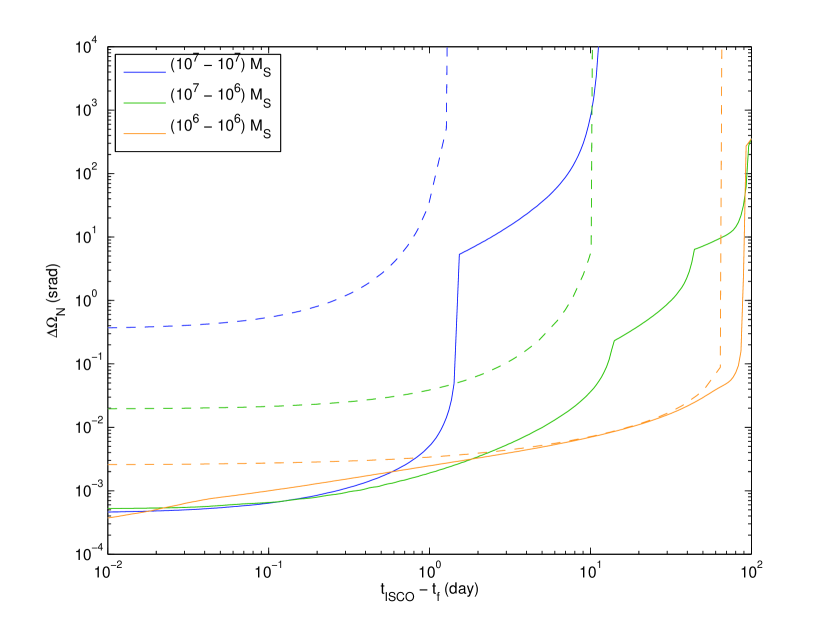
Figure 1: Time evolution of LISA’s angular resolution when we observe different supermassive black hole binary systems from one year before the merger up to $t_{f}$. Lookback time is represented the axis of abscissas, so time evolves from right to left. Fiducial sources are located at redshift $z=1$, with a common orientation defined by $\cos\theta_{L}=0.2$ and $\phi_{L}=3$ and a sky location of $\cos\theta_{N}=-0.383$ ; $\phi_{N}=2.82$. Solid lines correspond to FWF, and the dashed ones to RWF.

In order to issue warnings and search for electromagnetic counterparts, we need LISA to have enough angular resolution some time before the merger occurs. For this reason, we are not only interested in LISA’s angular resolution when we observe a source during the last year before merger, but also how the angular resolution evolves when we stop our observation some time before, and measure the importance of the FWF versus RWF. In figure 1 we study how the angular resolution is accumulated as a function of the lookback time, $t_{ISCO}-t_{f}$, for different sources located at $\cos\theta_{N}=-0.383$, $\phi_{N}=2.82$. Different sky locations have also been analyzed, see e.g. figure 14 in [18] for $\cos\theta_{N}=-0.6$, $\phi_{N}=1$. In this latter figure, we have that an angular resolution twice the final one is reached, respectively, $20$ days, $20$ hours and $8$ hours before merger, for binary systems of masses $(10^{6}-10^{6})~{}M_{\odot}$, $(10^{7}-10^{6})~{}M_{\odot}$ and $(10^{7}-10^{7})~{}M_{\odot}$. For the sky location considered here (figure 1), LISA’s angular resolution decreases more during the last days (hours) before merger, but we still are reaching almost the best angular resolution $12$ hours before merger. The jumps in the evolution of LISA’s angular resolution correspond to those times in which a new harmonic enters into the LISA band and it is related to the the low-frequency cut-off we have assumed for the instrument at $5\times 10^{-5}$ Hz. For equal masses, only the even multipoles of the orbital frequency contribute to the FWF, while for the unequal masses there is contribution from all the harmonics. For example, in the $10^{7}M_{\odot}-10^{7}M_{\odot}$ case the contribution of the 4th harmonic becomes relevant around 10 days before coalescence (independently of the sky location considered) while the 2nd harmonic rapidly increases the angular resolution 2 days before coalescence. For the unequal mass case $10^{7}M_{\odot}-10^{6}M_{\odot}$ we clearly see the contributions of the 2nd, 3rd and 4th harmonics.

Table 3: Comparison between median values of the probability distributions when we see LISA as a single Michelson interferometer or as a combination of two independent ones. Gain factors are computed in the same way as in table 1 and by loss we mean the factor that the errors get multiplied by (and the SNR divided by) when we lose one of the LISA’s arms.

	Detector $I$			Detector $I+II$			Loss
	$x_{50\%}$			$\quad x_{50\%}$
$x$	rwf	fwf	Gain	rwf	fwf	Gain	rwf	fwf
	(a) $m_{1}=10^{7}M_{\odot}$ ; $m_{2}=10^{6}M_{\odot}$
SNR	$161$	$152$	$0.94$	$231$	$212$	$0.92$	$1.4$	$1.4$
$\log_{10}\Delta\Omega_{N}/$srad	$3.40$	$-0.69$	$12000$	$-1.47$	$-2.46$	$9.7$	$74000$	$59$
$\log_{10}\Delta\Omega_{L}/$srad	$3.95$	$-0.89$	$69000$	$-1.14$	$-2.39$	$18$	$120000$	$32$
$\log_{10}\Delta D_{L}/D_{L}$	$1.84$	$-0.69$	$330$	$-0.60$	$-1.41$	$6.4$	$276$	$5.2$
$\log_{10}\Delta t_{c}/$s	$4.68$	$3.02$	$46$	$4.10$	$2.84$	$18$	$3.9$	$1.5$
$\log_{10}\Delta\mathcal{M}/\mathcal{M}$	$0.05$	$-2.46$	$320$	$-0.71$	$-2.66$	$88$	$5.8$	$1.6$
$\log_{10}\Delta\mu/\mu$	$1.70$	$-1.52$	$1700$	$1.00$	$-1.79$	$610$	$5.0$	$1.8$
	(b) $m_{1}=10^{6}M_{\odot}$ ; $m_{2}=10^{6}M_{\odot}$
SNR	$257$	$229$	$0.89$	$362$	$328$	$0.90$	$1.4$	$1.4$
$\log_{10}\Delta\Omega_{N}/$srad	$-0.96$	$-1.56$	$4.0$	$-2.42$	$-2.72$	$2.0$	$29$	$14$
$\log_{10}\Delta\Omega_{L}/$srad	$-0.19$	$-1.47$	$19$	$-2.15$	$-2.38$	$1.7$	$92$	$8.0$
$\log_{10}\Delta D_{L}/D_{L}$	$-0.39$	$-1.05$	$4.6$	$-1.37$	$-1.58$	$1.6$	$9.6$	$3.4$
$\log_{10}\Delta t_{c}/$s	$2.16$	$1.70$	$2.9$	$1.82$	$1.38$	$2.8$	$2.2$	$2.1$
$\log_{10}\Delta\mathcal{M}/\mathcal{M}$	$-2.30$	$-3.36$	$12$	$-2.66$	$-3.63$	$9.3$	$2.3$	$1.9$
$\log_{10}\Delta\mu/\mu$	$-0.14$	$-3.36$	$1700$	$-0.48$	$-3.63$	$1400$	$2.2$	$1.9$
	(c) $m_{1}=10^{6}M_{\odot}$ ; $m_{2}=10^{5}M_{\odot}$
SNR	$219$	$235$	$1.1$	$311$	$322$	$1.0$	$1.4$	$1.4$
$\log_{10}\Delta\Omega_{N}/$srad	$-1.75$	$-1.97$	$1.7$	$-2.51$	$-3.00$	$3.0$	$5.8$	$11$
$\log_{10}\Delta\Omega_{L}/$srad	$-0.96$	$-2.08$	$13$	$-2.23$	$-2.99$	$5.9$	$18$	$8.2$
$\log_{10}\Delta D_{L}/D_{L}$	$-0.79$	$-1.36$	$3.7$	$-1.41$	$-1.79$	$2.4$	$4.2$	$2.7$
$\log_{10}\Delta t_{c}/$s	$1.76$	$1.38$	$2.4$	$1.56$	$1.10$	$2.9$	$1.6$	$1.9$
$\log_{10}\Delta\mathcal{M}/\mathcal{M}$	$-3.06$	$-3.86$	$6.3$	$-3.27$	$-4.05$	$6.0$	$1.6$	$1.6$
$\log_{10}\Delta\mu/\mu$	$-1.03$	$-2.02$	$10$	$-1.24$	$-2.25$	$10$	$1.6$	$1.7$

Up to this point, we have considered LISA as two independent Michelson interferometers, using the long wavelength approximation, and we have provided the measurement errors for this two-detector case. But it is also interesting to study which is the impact on parameter estimation for a single interferometer. This is relevant in the hypothetical case that LISA would lose one of its arm links, in which case it would be interesting to know how LISA’s parameter estimation gets reduced and whether the effect is the same when we use the RWF model or the FWF one.

In table 3, we give the $50~{}\%$ levels of the cumulative probability distributions working with both RWF and FWF, for the single detector and the two-detector case. As one would expect, each of the independent interferometers measures, in average, similar values of SNR, and since $\rho^{tot}=\sqrt{(\rho^{I})^{2}+(\rho^{II})^{2}}$, losing one of LISA’s link means that the SNR gets reduced by a factor $\sqrt{2}$ in all cases. For the measurement errors, we see that in most of the cases (especially for high mass systems) the loss factor (i.e. the factor that errors have to be multiplied by when LISA loses one of its links) is higher for the RWF case, which means that working with the FWF not only improves LISA’s parameter estimation as we have seen before, but also reduces the impact of losing one arm link. In any case, even working with the FWF model, we see that losing one arm, means reducing the angular resolution by more than one order of magnitude, thus we will lose any possibility of observing the potential electromagnetic counterpart of the merger. Losses in the other parameters are not so serious: errors in the distance get multiplied by a factor $2-5$ and in masses by less than $2$.

4 Summary and outlook

This work clearly shows that modeling the inspiral with the full post-Newtonian waveform, as compared to the restricted-PN one, improves in general the parameter estimation of supermassive black hole systems, due to the much greater richness of the waveform. One should notice that the results presented here are influenced by a number of assumptions associated to these observations, in particular, the instrumental and confusion noise models we have adopted, the post-Newtonian waveform model and how this is terminated, and the lower-frequency cut-off we have imposed. The parameter estimation code we use has been validated by the LISA science performance evaluation taskforce [24]. This new taskforce, created at the September’07 LISA International Science Team meeting, is currently extending these results to include spin-induced precession into the full waveform and compare LISA’s science reach for different mission configurations, based also on astrophysically motivated source distributions [25]. It will be very interesting to extend these analyses using different post-Newtonian models and also to study parameter estimation for all three stages of the signal, including the merger and the ringdown, and use currently available phenomenological and numerical waveforms for that.

References

References

- [1] K. Danzmann et al., ”LISA Laser Interferometer Space Antenna, Pre-Phase A Report,” Max-Planck-Institut für Quantenoptic, Report No. MPQ 233, 1998 (unpublished).
- [2] K. Danzmann and A. Rüdiger, Class. Quant. Grav. 20, S1 (2003)
- [3] S. A. Hughes, Mon.ºNot.ºRoy.ºAstron.ºSoc.º 331, 805 (2002)
- [4] K. Menou, Z. Haiman and V. K. Narayanan, Astrophys.ºJ.º 558, 535 (2001)
- [5] O. Dreyer, B. Kelly, B. Krishnan, L. S. Finn, D. Garrison and R. Lopez-Aleman, Class.ºQuant.ºGrav.º 21, 787 (2004)
- [6] M. C. Miller, Astrophys.ºJ.º 618, 426 (2004)
- [7] S. A. Hughes and K. Menou, Astrophys.ºJ.º 623, 689 (2005)
- [8] E. Berti, A. Buonanno and C. M. Will, Phys.ºRev.º D 71, 084025 (2005)
- [9] K. G. Arun, B. R. Iyer, M. S. S. Qusailah and B. S. Sathyaprakash, Class.ºQuant.ºGrav.º 23, L37 (2006)
- [10] K. G. Arun, B. R. Iyer, M. S. S. Qusailah and B. S. Sathyaprakash, Phys.ºRev.º D 74, 024006 (2006)
- [11] B. F. Schutz, Nature 323, 310 (1986).
- [12] B. Kocsis, Z. Frei, Z. Haiman and K. Menou, Astrophys.ºJ.º 637, 27 (2006)
- [13] B. Kocsis, Z. Haiman, K. Menou and Z. Frei, Phys.ºRev.º D 76, 022003 (2007).
- [14] D. E. Holz and S. A. Hughes, Astrophys.ºJ.º 629, 15 (2005)
- [15] C. Cutler, Phys.ºRev.º D 57, 7089 (1998)
- [16] K. G. Arun, B. R. Iyer, B. S. Sathyaprakash and S. Sinha, Phys.ºRev.º D 75, 124002 (2007)
- [17] K. G. Arun, B. R. Iyer, B. S. Sathyaprakash, S. Sinha and C. V. D. Broeck, Phys.ºRev.º D 76, 104016 (2007) [Erratum-ibid.º D 76, 129903 (2007)]
- [18] M. Trias and A. M. Sintes, Phys.ºRev.º D 77, 024030 (2008)
- [19] L. Blanchet, Living Rev.ºRel.º 9, 4 (2006), available from http://www.livingreviews.org/lrr-2006-4
- [20] L. Blanchet, B. R. Iyer, C. M. Will and A. G. Wiseman, Class.ºQuant.ºGrav.º 13, 575 (1996)
- [21] K. G. Arun, L. Blanchet, B. R. Iyer and M. S. S. Qusailah, Class.ºQuant.ºGrav.º 21 (2004) 3771 [Erratum-ibid.º 22 (2005) 3115]
- [22] L. Barack and C. Cutler, Phys.ºRev.º D 70, 122002 (2004)
- [23] B. Kocsis, Z. Haiman and K. Menou, arXiv:0712.1144v1 [astro-ph]
- [24] http://www.tapir.caltech.edu/dokuwiki/lisape:home
- [25] E. Berti and M. Volonteri, arXiv:0802.0025 [astro-ph].