An introduction to Lévy processes
with applications in Finance

Abstract.

These lectures notes aim at introducing Lévy processes in an informal and intuitive way, accessible to non-specialists in the field. In the first part, we focus on the theory of Lévy processes. We analyze a ‘toy’ example of a Lévy process, viz. a Lévy jump-diffusion, which yet offers significant insight into the distributional and path structure of a Lévy process. Then, we present several important results about Lévy processes, such as infinite divisibility and the Lévy-Khintchine formula, the Lévy-Itô decomposition, the Itô formula for Lévy processes and Girsanov’s transformation. Some (sketches of) proofs are presented, still the majority of proofs is omitted and the reader is referred to textbooks instead. In the second part, we turn our attention to the applications of Lévy processes in financial modeling and option pricing. We discuss how the price process of an asset can be modeled using Lévy processes and give a brief account of market incompleteness. Popular models in the literature are presented and revisited from the point of view of Lévy processes, and we also discuss three methods for pricing financial derivatives. Finally, some indicative evidence from applications to market data is presented.

Part I Theory

1. Introduction

Lévy processes play a central role in several fields of science, such as physics, in the study of turbulence, laser cooling and in quantum field theory; in engineering, for the study of networks, queues and dams; in economics, for continuous time-series models; in the actuarial science, for the calculation of insurance and re-insurance risk; and, of course, in mathematical finance. A comprehensive overview of several applications of Lévy processes can be found in Prabhu98, in Barndorff-NielsenMikoschResnick01, in KyprianouSchoutensWilmott05 and in Kyprianou06.

In mathematical finance, Lévy processes are becoming extremely fashionable because they can describe the observed reality of financial markets in a more accurate way than models based on Brownian motion. In the ‘real’ world, we observe that asset price processes have jumps or spikes, and risk managers have to take them into consideration; in Figure 1.1 we can observe some big price changes (jumps) even on the very liquid USD/JPY exchange rate. Moreover, the empirical distribution of asset returns exhibits fat tails and skewness, behavior that deviates from normality; see Figure 1.2 for a characteristic picture. Hence, models that accurately fit return distributions are essential for the estimation of profit and loss (P&L) distributions. Similarly, in the ‘risk-neutral’ world, we observe that implied volatilities are constant neither across strike nor across maturities as stipulated by the BlackScholes73 (actually, Samuelson65) model; Figure 1.3 depicts a typical volatility surface. Therefore, traders need models that can capture the behavior of the implied volatility smiles more accurately, in order to handle the risk of trades. Lévy processes provide us with the appropriate tools to adequately and consistently describe all these observations, both in the ‘real’ and in the ‘risk-neutral’ world.

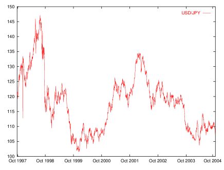
Figure 1.1. USD/JPY exchange rate, Oct. 1997–Oct. 2004.

The main aim of these lecture notes is to provide an accessible overview of the field of Lévy processes and their applications in mathematical finance to the non-specialist reader. To serve that purpose, we have avoided most of the proofs and only sketch a number of proofs, especially when they offer some important insight to the reader. Moreover, we have put emphasis on the intuitive understanding of the material, through several pictures and simulations.

We begin with the definition of a Lévy process and some known examples. Using these as the reference point, we construct and study a Lévy jump-diffusion; despite its simple nature, it offers significant insights and an intuitive understanding of general Lévy processes. We then discuss infinitely divisible distributions and present the celebrated Lévy–Khintchine formula, which links processes to distributions. The opposite way, from distributions to processes, is the subject of the Lévy-Itô decomposition of a Lévy process. The Lévy measure, which is responsible for the richness of the class of Lévy processes, is studied in some detail and we use it to draw some conclusions about the path and moment properties of a Lévy process. In the next section, we look into several subclasses that have attracted special attention and then present some important results from semimartingale theory. A study of martingale properties of Lévy processes and the Itô formula for Lévy processes follows. The change of probability measure and Girsanov’s theorem are studied is some detail and we also give a complete proof in the case of the Esscher transform. Next, we outline three ways for constructing new Lévy processes and the first part closes with an account on simulation methods for some Lévy processes.

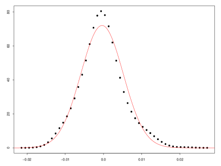
Figure 1.2. Empirical distribution of daily log-returns for the GBP/USD exchange rate and fitted Normal distribution.

The second part of the notes is devoted to the applications of Lévy processes in mathematical finance. We describe the possible approaches in modeling the price process of a financial asset using Lévy processes under the ‘real’ and the ‘risk-neutral’ world, and give a brief account of market incompleteness which links the two worlds. Then, we present a primer of popular Lévy models in the mathematical finance literature, listing some of their key properties, such as the characteristic function, moments and densities (if known). In the next section, we give an overview of three methods for pricing options in Lévy-driven models, viz. transform, partial integro-differential equation (PIDE) and Monte Carlo methods. Finally, we present some empirical results from the application of Lévy processes to real market financial data. The appendices collect some results about Poisson random variables and processes, explain some notation and provide information and links regarding the data sets used.

Naturally, there is a number of sources that the interested reader should consult in order to deepen his knowledge and understanding of Lévy processes. We mention here the books of Bertoin96, Sato99, Applebaum Applebaum04, Kyprianou06 on various aspects of Lévy processes. Cont and Tankov ContTankov03 and Schoutens03 focus on the applications of Lévy processes in finance. The books of JacodShiryaev03 and Protter Protter04 are essential readings for semimartingale theory, while Shiryaev99 blends semimartingale theory and applications to finance in an impressive manner. Other interesting and inspiring sources are the papers by Eberlein01a, Cont01, Barndorff-NielsenPrause01, Carr et al. Carretal02, Eberlein and ÖzkanEberleinOezkan03 and Eberlein07.

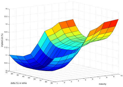
Figure 1.3. Implied volatilities of vanilla options on the EUR/USD exchange rate on November 5, 2001.

2. Definition

Let ($\Omega,\mathcal{F},\mathbf{F},P$) be a filtered probability space, where $\mathcal{F}=\mathcal{F}_{T}$ and the filtration $\mathbf{F}=(\mathcal{F}_{t})_{t\in[0,T]}$ satisfies the usual conditions. Let $T\in[0,\infty]$ denote the time horizon which, in general, can be infinite.

Definition 2.1.

A càdlàg, adapted, real valued stochastic process $L=(L_{t})_{0\leq t\leq T}$ with $L_{0}=0$ a.s. is called a Lévy process if the following conditions are satisfied:

(L1):

$L$ has independent increments, i.e. $L_{t}-L_{s}$ is independent of $\mathcal{F}_{s}$ for any $0\leq s<t\leq T$.

(L2):

$L$ has stationary increments, i.e. for any $0\leq s,t\leq T$ the distribution of $L_{t+s}-L_{t}$ does not depend on $t$.

(L3):

$L$ is stochastically continuous, i.e. for every ${0\leq t\leq T}$ and $\epsilon>0$: $\lim_{s\rightarrow t}P(|L_{t}-L_{s}|>\epsilon)=0$.

The simplest Lévy process is the linear drift, a deterministic process. Brownian motion is the only (non-deterministic) Lévy process with continuous sample paths.

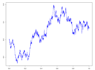
Figure 2.4. Examples of Lévy processes: linear drift (left) and Brownian motion.

Other examples of Lévy processes are the Poisson and compound Poisson processes. Notice that the sum of a linear drift, a Brownian motion and a compound Poisson process is again a Lévy process; it is often called a “jump-diffusion” process. We shall call it a “Lévy jump-diffusion” process, since there exist jump-diffusion processes which are not Lévy processes.

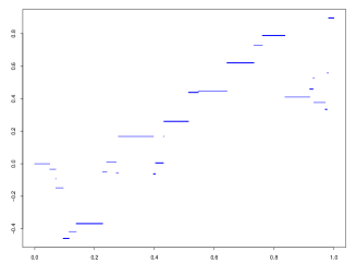
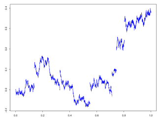
Figure 2.5. Examples of Lévy processes: compound Poisson process (left) and Lévy jump-diffusion.

3. ‘Toy’ example: a Lévy jump-diffusion

Assume that the process $L=(L_{t})_{0\leq t\leq T}$ is a Lévy jump-diffusion, i.e. a Brownian motion plus a compensated compound Poisson process. The paths of this process can be described by

(3.1) $$L_{t}=bt+\sigma W_{t}+\Big{(}\sum_{k=1}^{N_{t}}J_{k}-t\lambda\kappa\Big{)}$$

where $b\in\mathbb{R}$, $\sigma\in\mathbb{R}_{\geqslant 0}$, $W=(W_{t})_{0\leq t\leq T}$ is a standard Brownian motion, $N=(N_{t})_{0\leq t\leq T}$ is a Poisson process with parameter $\lambda$ (i.e. $\mathrm{I\kern-1.99997ptE}[N_{t}]=\lambda t$) and $J=(J_{k})_{k\geq 1}$ is an i.i.d. sequence of random variables with probability distribution $F$ and $\mathrm{I\kern-1.99997ptE}[J]=\kappa<\infty$. Hence, $F$ describes the distribution of the jumps, which arrive according to the Poisson process. All sources of randomness are mutually independent.

It is well known that Brownian motion is a martingale; moreover, the compensated compound Poisson process is a martingale. Therefore, $L=(L_{t})_{0\leq t\leq T}$ is a martingale if and only if $b=0$.

The characteristic function of $L_{t}$ is

$$\mathrm{I\kern-1.99997ptE}\big{[}\mathrm{e}^{iuL_{t}}\big{]} =\mathrm{I\kern-1.99997ptE}\Big{[}\exp\big{(}iu\big{(}bt+\sigma W_{t}+\sum_{k=1}^{N_{t}}J_{k}-t\lambda\kappa\big{)}\big{)}\Big{]}$$

$$=\exp\big{[}iubt\big{]}\mathrm{I\kern-1.99997ptE}\Big{[}\exp\big{(}iu\sigma W_{t}\big{)}\exp\big{(}iu\big{(}\sum_{k=1}^{N_{t}}J_{k}-t\lambda\kappa\big{)}\big{)}\Big{]};$$

since all the sources of randomness are independent, we get

$$=\exp\big{[}iubt\big{]}\mathrm{I\kern-1.99997ptE}\Big{[}\exp\big{(}iu\sigma W_{t}\big{)}\Big{]}\mathrm{I\kern-1.99997ptE}\Big{[}\exp\big{(}iu\sum_{k=1}^{N_{t}}J_{k}-iut\lambda\kappa\big{)}\Big{]};$$

$$=\exp\big{[}iubt\big{]}\exp\Big{[}-\frac{1}{2}u^{2}\sigma^{2}t\Big{]}\exp\Big{[}\lambda t\big{(}\mathrm{I\kern-1.99997ptE}[\mathrm{e}^{iuJ}-1]-iu\mathrm{I\kern-1.99997ptE}[J]\big{)}\Big{]}$$

$$=\exp\big{[}iubt\big{]}\exp\Big{[}-\frac{1}{2}u^{2}\sigma^{2}t\Big{]}\exp\Big{[}\lambda t\big{(}\mathrm{I\kern-1.99997ptE}[\mathrm{e}^{iuJ}-1-iuJ]\big{)}\Big{]};$$

and because the distribution of $$J F$$ is we have

$$=\exp\big{[}iubt\big{]}\exp\Big{[}-\frac{1}{2}u^{2}\sigma^{2}t\Big{]}\exp\Big{[}\lambda t\int_{\mathbb{R}}\big{(}\mathrm{e}^{iux}-1-iux\big{)}F(\mathrm{d}x)\Big{]}.$$

Now, since $t$ is a common factor, we re-write the above equation as

(3.2) $$\mathrm{I\kern-1.99997ptE}\big{[}\mathrm{e}^{iuL_{t}}\big{]}=\exp\bigg{[}t\Big{(}iub-\frac{u^{2}\sigma^{2}}{2}+\int_{\mathbb{R}}(\mathrm{e}^{iux}-1-iux)\lambda F(\mathrm{d}x)\Big{)}\bigg{]}.$$

Since the characteristic function of a random variable determines its distribution, we have a “characterization” of the distribution of the random variables underlying the Lévy jump-diffusion. We will soon see that this distribution belongs to the class of infinitely divisible distributions and that equation (3.2) is a special case of the celebrated Lévy-Khintchine formula.

Remark 3.1.

Note that time factorizes out, and the drift, diffusion and jumps parts are separated; moreover, the jump part factorizes to expected number of jumps ($\lambda$) and distribution of jump size ($F$). It is only natural to ask if these features are preserved for all Lévy processes. The answer is yes for the first two questions, but jumps cannot be always separated into a product of the form $\lambda\times F$.

4. Infinitely divisible distributions and the Lévy-Khintchine formula

There is a strong interplay between Lévy processes and infinitely divisible distributions. We first define infinitely divisible distributions and give some examples, and then describe their relationship to Lévy processes.

Let $X$ be a real valued random variable, denote its characteristic function by $\varphi_{X}$ and its law by $P_{X}$, hence $\varphi_{X}(u)=\int_{\mathbb{R}}\mathrm{e}^{iux}P_{X}(\mathrm{d}x)$. Let $\mu*\nu$ denote the convolution of the measures $\mu$ and $\nu$, i.e. $(\mu*\nu)(A)=\int_{\mathbb{R}}\nu(A-x)\mu(\mathrm{d}x)$.

Definition 4.1.

The law $P_{X}$ of a random variable $X$ is infinitely divisible, if for all $n\in\mathbb{N}$ there exist i.i.d. random variables $X^{(1/n)}_{1},\ldots,X^{(1/n)}_{n}$ such that

(4.1) $$X\stackrel{{\scriptstyle\mathrm{d}}}{{=}}X^{(1/n)}_{1}+\ldots+X^{(1/n)}_{n}.$$

Equivalently, the law $P_{X}$ of a random variable $X$ is infinitely divisible if for all $n\in\mathbb{N}$ there exists another law $P_{X^{(1/n)}}$ of a random variable $X^{(1/n)}$ such that

(4.2) $$P_{X}=\underbrace{P_{X^{(1/n)}}*\ldots*P_{X^{(1/n)}}}_{n\;\text{times}}.$$

Alternatively, we can characterize an infinitely divisible random variable using its characteristic function.

Characterization 4.2.

The law of a random variable $X$ is infinitely divisible, if for all $n\in\mathbb{N}$, there exists a random variable $X^{(1/n)}$, such that

(4.3) $$\varphi_{X}(u)=\Big{(}\varphi_{X^{(1/n)}}(u)\Big{)}^{n}.$$

Example 4.3 (Normal distribution).

Using the characterization above, we can easily deduce that the Normal distribution is infinitely divisible. Let $X\sim\text{Normal}(\mu,\sigma^{2})$, then we have

$$\varphi_{X}(u) =\exp\Big{[}iu\mu-\frac{1}{2}u^{2}\sigma^{2}\Big{]}=\exp\Big{[}n(iu\frac{\mu}{n}-\frac{1}{2}u^{2}\frac{\sigma^{2}}{n})\Big{]}$$

$$=\Bigg{(}\exp\Big{[}iu\frac{\mu}{n}-\frac{1}{2}u^{2}\frac{\sigma^{2}}{n}\Big{]}\Bigg{)}^{n}$$

$$=\Big{(}\varphi_{X^{(1/n)}}(u)\Big{)}^{n},$$

where $X^{(1/n)}\sim\text{Normal}(\frac{\mu}{n},\frac{\sigma^{2}}{n})$.

Example 4.4 (Poisson distribution).

Following the same procedure, we can easily conclude that the Poisson distribution is also infinitely divisible. Let $X\sim\text{Poisson}(\lambda)$, then we have

$$\varphi_{X}(u) =\exp\Big{[}\lambda(\mathrm{e}^{iu}-1)\Big{]}=\Bigg{(}\exp\Big{[}\frac{\lambda}{n}(\mathrm{e}^{iu}-1)\Big{]}\Bigg{)}^{n}$$

$$=\Big{(}\varphi_{X^{(1/n)}}(u)\Big{)}^{n},$$

where $X^{(1/n)}\sim\text{Poisson}(\frac{\lambda}{n})$.

Remark 4.5.

Other examples of infinitely divisible distributions are the compound Poisson distribution, the exponential, the $\Gamma$-distribution, the geometric, the negative binomial, the Cauchy distribution and the strictly stable distribution. Counter-examples are the uniform and binomial distributions.

The next theorem provides a complete characterization of random variables with infinitely divisible distributions via their characteristic functions; this is the celebrated Lévy-Khintchine formula. We will use the following preparatory result (cf. [Lemma 7.8]Sato99).

Lemma 4.6.

If $(P_{k})_{k\geq 0}$ is a sequence of infinitely divisible laws and $P_{k}\rightarrow P$, then $P$ is also infinitely divisible.

Theorem 4.7.

The law $P_{X}$ of a random variable $X$ is infinitely divisible if and only if there exists a triplet $(b,c,\nu)$, with $b\in\mathbb{R}$, $c\in\mathbb{R}_{\geqslant 0}$ and a measure satisfying $\nu(\{0\})=0$ and $\int_{\mathbb{R}}(1\wedge|x|^{2})\nu(\mathrm{d}x)<\infty$, such that

(4.4) $$\mathrm{I\kern-1.99997ptE}[\mathrm{e}^{iuX}]=\exp\Big{[}ibu-\frac{u^{2}c}{2}+\int_{\mathbb{R}}(\mathrm{e}^{iux}-1-iux1_{\{|x|<1\}})\nu(\mathrm{d}x)\Big{]}.$$

Sketch of Proof.

Here we describe the proof of the “if” part, for the full proof see Theorem 8.1 in Sato99. Let $(\varepsilon_{n})_{n\in\mathbb{N}}$ be a sequence in $\mathbb{R}$, monotonic and decreasing to zero. Define for all $u\in\mathbb{R}$ and $n\in\mathbb{N}$

$$\varphi_{X_{n}}(u)=\exp\Big{[}iu\Big{(}b-\!\!\int_{\varepsilon_{n}<|x|\leq 1}\!\!x\nu(\mathrm{d}x)\Big{)}-\frac{u^{2}c}{2}+\int_{|x|>\varepsilon_{n}}(\mathrm{e}^{iux}-1)\nu(\mathrm{d}x)\Big{]}.$$

Each $\varphi_{X_{n}}$ is the convolution of a normal and a compound Poisson distribution, hence $\varphi_{X_{n}}$ is the characteristic function of an infinitely divisible probability measure $P_{X_{n}}$. We clearly have that

$$\lim_{n\rightarrow\infty}\varphi_{X_{n}}(u)=\varphi_{X}(u);$$

then, by Lévy’s continuity theorem and Lemma 4.6, $\varphi_{X}$ is the characteristic function of an infinitely divisible law, provided that $\varphi_{X}$ is continuous at $0$.

Now, continuity of $\varphi_{X}$ at $0$ boils down to the continuity of the integral term, i.e.

$$\psi_{\nu}(u) =\int_{\mathbb{R}}(\mathrm{e}^{iux}-1-iux1_{\{|x|<1\}})\nu(\mathrm{d}x)$$

$$=\int_{\{|x|\leq 1\}}(\mathrm{e}^{iux}-1-iux)\nu(\mathrm{d}x)+\int_{\{|x|>1\}}(\mathrm{e}^{iux}-1)\nu(\mathrm{d}x).$$

Using Taylor’s expansion, the Cauchy–Schwarz inequality, the definition of the Lévy measure and dominated convergence, we get

$$|\psi_{\nu}(u)| \leq\frac{1}{2}\int_{\{|x|\leq 1\}}|u^{2}x^{2}|\nu(\mathrm{d}x)+\int_{\{|x|>1\}}|\mathrm{e}^{iux}-1|\nu(\mathrm{d}x)$$

$$\leq\frac{|u|^{2}}{2}\int_{\{|x|\leq 1\}}|x^{2}|\nu(\mathrm{d}x)+\int_{\{|x|>1\}}|\mathrm{e}^{iux}-1|\nu(\mathrm{d}x)$$

$$\longrightarrow 0\quad\text{as}\quad u\rightarrow 0.\qed$$

The triplet ($b,c,\nu$) is called the Lévy or characteristic triplet and the exponent in (4.4)

(4.5) $$\psi(u)=iub-\frac{u^{2}c}{2}+\int_{\mathbb{R}}(\mathrm{e}^{iux}-1-iux1_{\{|x|<1\}})\nu(\mathrm{d}x)$$

is called the Lévy or characteristic exponent. Moreover, $b\in\mathbb{R}$ is called the drift term, $c\in\mathbb{R}_{\geqslant 0}$ the Gaussian or diffusion coefficient and $\nu$ the Lévy measure.

Remark 4.8.

Comparing equations (3.2) and (4.4), we can immediately deduce that the random variable $L_{t}$ of the Lévy jump-diffusion is infinitely divisible with Lévy triplet $b=b\cdot t,c=\sigma^{2}\cdot t$ and $\nu=(\lambda F)\cdot t$.

Now, consider a Lévy process $L=(L_{t})_{0\leq t\leq T}$; for any $n\in\mathbb{N}$ and any $0<t\leq T$ we trivially have that

(4.6) $$L_{t}=L_{\frac{t}{n}}+(L_{\frac{2t}{n}}-L_{\frac{t}{n}})+\ldots+(L_{t}-L_{\frac{(n-1)t}{n}}).$$

The stationarity and independence of the increments yield that $(L_{\frac{tk}{n}}-L_{\frac{t(k-1)}{n}})_{k\geq 1}$ is an i.i.d. sequence of random variables, hence we can conclude that the random variable $L_{t}$ is infinitely divisible.

Theorem 4.9.

For every Lévy process $L=(L_{t})_{0\leq t\leq T}$, we have that

(4.7) $$\mathrm{I\kern-1.99997ptE}[\mathrm{e}^{iuL_{t}}] =\mathrm{e}^{t\psi(u)}$$

$$=\exp\Big{[}t\big{(}ibu-\frac{u^{2}c}{2}+\int_{\mathbb{R}}(\mathrm{e}^{iux}-1-iux1_{\{|x|<1\}})\nu(\mathrm{d}x)\big{)}\Big{]}$$

where $\psi(u)$ is the characteristic exponent of $L_{1}$, a random variable with an infinitely divisible distribution.

Sketch of Proof.

Define the function $\phi_{u}(t)=\varphi_{L_{t}}(u)$, then we have

(4.8) $$\phi_{u}(t+s) =\mathrm{I\kern-1.99997ptE}[\mathrm{e}^{iuL_{t+s}}]=\mathrm{I\kern-1.99997ptE}[\mathrm{e}^{iu(L_{t+s}-L_{s})}\mathrm{e}^{iuL_{s}}]$$

$$=\mathrm{I\kern-1.99997ptE}[\mathrm{e}^{iu(L_{t+s}-L_{s})}]\mathrm{I\kern-1.99997ptE}[\mathrm{e}^{iuL_{s}}]=\phi_{u}(t)\phi_{u}(s).$$

Now, $\phi_{u}(0)=1$ and the map $t\mapsto\phi_{u}(t)$ is continuous (by stochastic continuity). However, the unique continuous solution of the Cauchy functional equation (4.8) is

(4.9) $$\phi_{u}(t)=\mathrm{e}^{t\vartheta(u)},\qquad{\mathrm{where}}\qquad\vartheta:\mathbb{R}\rightarrow\mathbb{C}.$$

Since $L_{1}$ is an infinitely divisible random variable, the statement follows. ∎

We have seen so far, that every Lévy process can be associated with the law of an infinitely divisible distribution. The opposite, i.e. that given any random variable $X$, whose law is infinitely divisible, we can construct a Lévy process $L=(L_{t})_{0\leq t\leq T}$ such that $\mathcal{L}(L_{1}):=\mathcal{L}(X)$, is also true. This will be the subject of the Lévy-Itô decomposition. We prepare this result with an analysis of the jumps of a Lévy process and the introduction of Poisson random measures.

5. Analysis of jumps and Poisson random measures

The jump process $\Delta L=(\Delta L_{t})_{0\leq t\leq T}$ associated to the Lévy process $L$ is defined, for each ${0\leq t\leq T}$, via

$$\Delta L_{t}=L_{t}-L_{t-},$$

where $L_{t-}=\lim_{s\uparrow t}L_{s}$. The condition of stochastic continuity of a Lévy process yields immediately that for any Lévy process $L$ and any fixed $t>0$, then $\Delta L_{t}=0$ a.s.; hence, a Lévy process has no fixed times of discontinuity.

In general, the sum of the jumps of a Lévy process does not converge, in other words it is possible that

$$\sum_{s\leq t}|\Delta L_{s}|=\infty\quad\text{a.s.}$$

but we always have that

$$\sum_{s\leq t}|\Delta L_{s}|^{2}<\infty\quad\text{a.s.}$$

which allows us to handle Lévy processes by martingale techniques.

A convenient tool for analyzing the jumps of a Lévy process is the random measure of jumps of the process. Consider a set $A\in\mathcal{B}(\mathbb{R}\backslash\{0\})$ such that $0\notin\overline{A}$ and let $0\leq t\leq T$; define the random measure of the jumps of the process $L$ by

(5.1) $$\mu^{L}(\omega;t,A) =\#\{0\leq s\leq t;\Delta L_{s}(\omega)\in A\}$$

$$=\sum_{s\leq t}1_{A}(\Delta L_{s}(\omega));$$

hence, the measure $\mu^{L}(\omega;t,A)$ counts the jumps of the process $L$ of size in $A$ up to time $t$. Now, we can check that $\mu^{L}$ has the following properties:

$$\mu^{L}(t,A)-\mu^{L}(s,A)\in\sigma(\{L_{u}-L_{v};s\leq v<u\leq t\})$$

hence $\mu^{L}(t,A)-\mu^{L}(s,A)$ is independent of $\mathcal{F}_{s}$, i.e. $\mu^{L}(\cdot,A)$ has independent increments. Moreover, $\mu^{L}(t,A)-\mu^{L}(s,A)$ equals the number of jumps of $L_{s+u}-L_{s}$ in $A$ for $0\leq u\leq t-s$; hence, by the stationarity of the increments of $L$, we conclude:

$$\mathcal{L}(\mu^{L}(t,A)-\mu^{L}(s,A))=\mathcal{L}(\mu^{L}(t-s,A))$$

i.e. $\mu^{L}(\cdot,A)$ has stationary increments.

Hence, $\mu^{L}(\cdot,A)$ is a Poisson process and $\mu^{L}$ is a Poisson random measure. The intensity of this Poisson process is $\nu(A)=\mathrm{I\kern-1.99997ptE}[\mu^{L}(1,A)]$.

Theorem 5.1.

The set function $A\mapsto\mu^{L}(\omega;t,A)$ defines a $\sigma$-finite measure on $\mathbb{R}\backslash\{0\}$ for each $(\omega,t)$. The set function $\nu(A)=\mathrm{I\kern-1.99997ptE}[\mu^{L}(1,A)]$ defines a $\sigma$-finite measure on $\mathbb{R}\backslash\{0\}$.

Proof.

The set function $A\mapsto\mu^{L}(\omega;t,A)$ is simply a counting measure on $\mathcal{B}(\mathbb{R}\backslash\{0\})$; hence,

$$\mathrm{I\kern-1.99997ptE}[\mu^{L}(t,A)]=\int\mu^{L}(\omega;t,A)\mathrm{d}P(\omega)$$

is a Borel measure on $\mathcal{B}(\mathbb{R}\backslash\{0\})$. ∎

Definition 5.2.

The measure $\nu$ defined by

$$\nu(A)=\mathrm{I\kern-1.99997ptE}[\mu^{L}(1,A)]=\mathrm{I\kern-1.99997ptE}\big{[}\sum_{s\leq 1}1_{A}(\Delta L_{s}(\omega))\big{]}$$

is the Lévy measure of the Lévy process $L$.

Now, using that $\mu^{L}(t,A)$ is a counting measure we can define an integral with respect to the Poisson random measure $\mu^{L}$. Consider a set $A\in\mathcal{B}(\mathbb{R}\backslash\{0\})$ such that $0\notin\overline{A}$ and a function $f:\mathbb{R}\rightarrow\mathbb{R}$, Borel measurable and finite on $A$. Then, the integral with respect to a Poisson random measure is defined as follows:

(5.2) $$\int_{A}f(x)\mu^{L}(\omega;t,\mathrm{d}x)=\sum_{s\leq t}f(\Delta L_{s})1_{A}(\Delta L_{s}(\omega)).$$

Note that each $\int_{A}f(x)\mu^{L}(t,\mathrm{d}x)$ is a real-valued random variable and generates a càdlàg stochastic process. We will denote the stochastic process by $\int_{0}^{\cdot}\int_{A}f(x)\mu^{L}(\mathrm{d}s,\mathrm{d}x)=(\int_{0}^{t}\int_{A}f(x)\mu^{L}(\mathrm{d}s,\mathrm{d}x))_{0\leq t\leq T}$.

Theorem 5.3.

Consider a set $A\in\mathcal{B}(\mathbb{R}\backslash\{0\})$ with $0\notin\overline{A}$ and a function $f:\mathbb{R}\rightarrow\mathbb{R}$, Borel measurable and finite on $A$.

1. The process $(\int_{0}^{t}\int_{A}f(x)\mu^{L}(\mathrm{d}s,\mathrm{d}x))_{{0\leq t\leq T}}$ is a compound Poisson process with characteristic function

   (5.3) $$\mathrm{I\kern-1.99997ptE}\Big{[}\exp\Big{(}iu\int\nolimits_{0}^{t}\!\int\nolimits_{A}f(x)\mu^{L}(\mathrm{d}s,\mathrm{d}x)\Big{)}\Big{]}=\exp\Big{(}t\int\nolimits_{A}(\mathrm{e}^{iuf(x)}-1)\nu(\mathrm{d}x)\Big{)}.\vspace{-.5em}$$

1. If $f\in L^{1}(A)$, then

   (5.4) $$\mathrm{I\kern-1.99997ptE}\Big{[}\int\nolimits_{0}^{t}\!\int\nolimits_{A}f(x)\mu^{L}(\mathrm{d}s,\mathrm{d}x)\Big{]}=t\int\nolimits_{A}f(x)\nu(\mathrm{d}x).$$

1. If $f\in L^{2}(A)$, then

   (5.5) $$\mathrm{Var}\Big{(}\Big{|}\int\nolimits_{0}^{t}\!\int\nolimits_{A}f(x)\mu^{L}(\mathrm{d}s,\mathrm{d}x)\Big{|}\Big{)}=t\int\nolimits_{A}|f(x)|^{2}\nu(\mathrm{d}x).$$

Sketch of Proof.

The structure of the proof is to start with simple functions and pass to positive measurable functions, then take limits and use dominated convergence; cf. Theorem 2.3.8 in Applebaum04. ∎

6. The Lévy-Itô decomposition

Theorem 6.1.

Consider a triplet $(b,c,\nu)$ where $b\in\mathbb{R}$, $c\in\mathbb{R}_{\geqslant 0}$ and $\nu$ is a measure satisfying $\nu(\{0\})=0$ and $\int_{\mathbb{R}}(1\wedge|x|^{2})\nu(\mathrm{d}x)<\infty$. Then, there exists a probability space $(\Omega,\mathcal{F},P)$ on which four independent Lévy processes exist, $L^{(1)}$, $L^{(2)}$, $L^{(3)}$ and $L^{(4)}$, where $L^{(1)}$ is a constant drift, $L^{(2)}$ is a Brownian motion, $L^{(3)}$ is a compound Poisson process and $L^{(4)}$ is a square integrable (pure jump) martingale with an a.s. countable number of jumps of magnitude less than $1$ on each finite time interval. Taking $L=L^{(1)}+L^{(2)}+L^{(3)}+L^{(4)}$, we have that there exists a probability space on which a Lévy process $L=(L_{t})_{0\leq t\leq T}$ with characteristic exponent

(6.1) $$\psi(u)=iub-\frac{u^{2}c}{2}+\int_{\mathbb{R}}(\mathrm{e}^{iux}-1-iux1_{\{|x|<1\}})\nu(\mathrm{d}x)$$

for all $u\in\mathbb{R}$, is defined.

Proof.

See chapter 4 in Sato99 or chapter 2 in Kyprianou06. ∎

The Lévy-Itô decomposition is a hard mathematical result to prove; here, we go through some steps of the proof because it reveals much about the structure of the paths of a Lévy process. We split the Lévy exponent (6.1) into four parts

$$\psi=\psi^{(1)}+\psi^{(2)}+\psi^{(3)}+\psi^{(4)}$$

where

$$\psi^{(1)}(u) =iub,\qquad\psi^{(2)}(u)=\frac{u^{2}c}{2},$$

$$\psi^{(3)}(u) =\int_{|x|\geq 1}(\mathrm{e}^{iux}-1)\nu(\mathrm{d}x),$$

$$\psi^{(4)}(u) =\int_{|x|<1}(\mathrm{e}^{iux}-1-iux)\nu(\mathrm{d}x).$$

The first part corresponds to a deterministic linear process (drift) with parameter $b$, the second one to a Brownian motion with coefficient $\sqrt{c}$ and the third part corresponds to a compound Poisson process with arrival rate $\lambda:=\nu(\mathbb{R}\backslash(-1,1))$ and jump magnitude $F(\mathrm{d}x):=\frac{\nu(\mathrm{d}x)}{\nu(\mathbb{R}\setminus(-1,1))}1_{\{|x|\geq 1\}}$.

The last part is the most difficult to handle; let $\Delta L^{(4)}$ denote the jumps of the Lévy process $L^{(4)}$, that is $\Delta L^{(4)}_{t}=L^{(4)}_{t}-L^{(4)}_{t-}$, and let $\mu^{L^{(4)}}$ denote the random measure counting the jumps of $L^{(4)}$. Next, one constructs a compensated compound Poisson process

$$L^{(4,\epsilon)}_{t} =\sum_{0\leq s\leq t}\Delta L^{(4)}_{s}1_{\{1>|\Delta L^{(4)}_{s}|>\epsilon\}}-t\Big{(}\int_{1>|x|>\epsilon}x\nu(\mathrm{d}x)\Big{)}$$

$$=\int_{0}^{t}\int_{1>|x|>\epsilon}x\mu^{L^{(4)}}(\mathrm{d}x,\mathrm{d}s)-t\Big{(}\int_{1>|x|>\epsilon}x\nu(\mathrm{d}x)\Big{)}$$

and shows that the jumps of $L^{(4)}$ form a Poisson process; using Theorem 5.3 we get that the characteristic exponent of $L^{(4,\epsilon)}$ is

$$\psi^{(4,\epsilon)}(u) =\int_{\epsilon<|x|<1}(\mathrm{e}^{iux}-1-iux)\nu(\mathrm{d}x).$$

Then, there exists a Lévy process $L^{(4)}$ which is a square integrable martingale, such that $L^{(4,\epsilon)}\rightarrow L^{(4)}$ uniformly on $[0,T]$ as $\epsilon\rightarrow 0+$. Clearly, the Lévy exponent of the latter Lévy process is $\psi^{(4)}$.

Therefore, we can decompose any Lévy process into four independent Lévy processes $L=L^{(1)}+L^{(2)}+L^{(3)}+L^{(4)}$, as follows

(6.2) $$L_{t} =bt+\sqrt{c}W_{t}+\int_{0}^{t}\int_{|x|\geq 1}x\mu^{L}(\mathrm{d}s,\mathrm{d}x)+\int_{0}^{t}\int_{|x|<1}x(\mu^{L}-\nu^{L})(\mathrm{d}s,\mathrm{d}x)$$

where $\nu^{L}(\mathrm{d}s,\mathrm{d}x)=\nu(\mathrm{d}x)\mathrm{d}s$. Here $L^{(1)}$ is a constant drift, $L^{(2)}$ a Brownian motion, $L^{(3)}$ a compound Poisson process and $L^{(4)}$ a pure jump martingale. This result is the celebrated Lévy-Itô decomposition of a Lévy process.

7. The Lévy measure, path and moment properties

The Lévy measure $\nu$ is a measure on $\mathbb{R}$ that satisfies

(7.1) $$\nu(\{0\})=0 \qquad\mathrm{and} \qquad\int_{\mathbb{R}}(1\wedge|x|^{2})\nu(\mathrm{d}x)<\infty.$$

Intuitively speaking, the Lévy measure describes the expected number of jumps of a certain height in a time interval of length 1. The Lévy measure has no mass at the origin, while singularities (i.e. infinitely many jumps) can occur around the origin (i.e. small jumps). Moreover, the mass away from the origin is bounded (i.e. only a finite number of big jumps can occur).

Recall the example of the Lévy jump-diffusion; the Lévy measure is $\nu(\mathrm{d}x)=\lambda\times F(\mathrm{d}x)$; from that we can deduce that the expected number of jumps is $\lambda$ and the jump size is distributed according to $F$.

More generally, if $\nu$ is a finite measure, i.e. $\lambda:=\nu(\mathbb{R})=\int_{\mathbb{R}}\nu(\mathrm{d}x)<\infty$, then we can define $F(\mathrm{d}x):=\frac{\nu(\mathrm{d}x)}{\lambda}$, which is a probability measure. Thus, $\lambda$ is the expected number of jumps and $F(\mathrm{d}x)$ the distribution of the jump size $x$. If $\nu(\mathbb{R})=\infty$, then an infinite number of (small) jumps is expected.

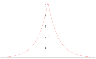
Figure 7.6. The distribution function of the Lévy measure of the standard Poisson process (left) and the density of the Lévy measure of a compound Poisson process with double-exponentially distributed jumps.

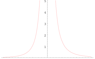
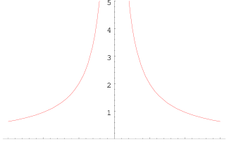
Figure 7.7. The density of the Lévy measure of an NIG (left) and an $\alpha$-stable process.

The Lévy measure is responsible for the richness of the class of Lévy processes and carries useful information about the structure of the process. Path properties can be read from the Lévy measure: for example, Figures 7.6 and 7.7 reveal that the compound Poisson process has a finite number of jumps on every time interval, while the NIG and $\alpha$-stable processes have an infinite one; we then speak of an infinite activity Lévy process.

Proposition 7.1.

Let $L$ be a Lévy process with triplet $(b,c,\nu)$.

1. If $\nu(\mathbb{R})<\infty$, then almost all paths of $L$ have a finite number of jumps on every compact interval. In that case, the Lévy process has finite activity.

2. If $\nu(\mathbb{R})=\infty$, then almost all paths of $L$ have an infinite number of jumps on every compact interval. In that case, the Lévy process has infinite activity.

Proof.

See Theorem 21.3 in Sato99. ∎

Whether a Lévy process has finite variation or not also depends on the Lévy measure (and on the presence or absence of a Brownian part).

Proposition 7.2.

Let $L$ be a Lévy process with triplet $(b,c,\nu)$.

1. If $c=0$ and $\int_{|x|\leq 1}|x|\nu(\mathrm{d}x)<\infty$, then almost all paths of $L$ have finite variation.

2. If $c\neq 0$ or $\int_{|x|\leq 1}|x|\nu(\mathrm{d}x)=\infty$, then almost all paths of $L$ have infinite variation.

Proof.

See Theorem 21.9 in Sato99. ∎

The different functions a Lévy measure has to integrate in order to have finite activity or variation, are graphically exhibited in Figure 7.8. The compound Poisson process has finite measure, hence it has finite variation as well; on the contrary, the NIG Lévy process has an infinite measure and has infinite variation. In addition, the CGMY Lévy process for $0<Y<1$ has infinite activity, but the paths have finite variation.

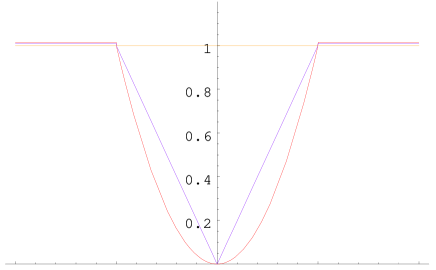
Figure 7.8. The Lévy measure must integrate $|x|^{2}\wedge 1$ (red line); it has finite variation if it integrates $|x|\wedge 1$ (blue line); it is finite if it integrates $1$ (orange line).

The Lévy measure also carries information about the finiteness of the moments of a Lévy process. This is particularly useful information in mathematical finance, related to the existence of a martingale measure.

The finiteness of the moments of a Lévy process is related to the finiteness of an integral over the Lévy measure (more precisely, the restriction of the Lévy measure to jumps larger than $1$ in absolute value, i.e. big jumps).

Proposition 7.3.

Let $L$ be a Lévy process with triplet $(b,c,\nu)$. Then

1. $L_{t}$ has finite $p$-th moment for $p\in\mathbb{R}_{\geqslant 0}$ $(\mathrm{I\kern-1.99997ptE}|L_{t}|^{p}<\infty)$ if and only if $\int_{|x|\geq 1}|x|^{p}\nu(\mathrm{d}x)<\infty$.

2. $L_{t}$ has finite $p$-th exponential moment for $p\in\mathbb{R}$ $(\mathrm{I\kern-1.99997ptE}[\mathrm{e}^{pL_{t}}]<\infty)$ if and only if $\int_{|x|\geq 1}\mathrm{e}^{px}\nu(\mathrm{d}x)<\infty$.

Proof.

The proof of these results can be found in Theorem 25.3 in Sato99. Actually, the conclusion of this theorem holds for the general class of submultiplicative functions (cf. Definition 25.1 in Sato99), which contains $\exp(px)$ and $|x|^{p}\vee 1$ as special cases. ∎

In order to gain some understanding of this result and because it blends beautifully with the Lévy-Itô decomposition, we will give a rough proof of the sufficiency for the second statement (inspired by Kyprianou06).

Recall from the Lévy-Itô decomposition, that the characteristic exponent of a Lévy process was split into four independent parts, the third of which is a compound Poisson process with arrival rate $\lambda:=\nu(\mathbb{R}\backslash(-1,1))$ and jump magnitude $F(\mathrm{d}x):=\frac{\nu(\mathrm{d}x)}{\nu(\mathbb{R}\backslash(-1,1))}1_{\{|x|\geq 1\}}$. Finiteness of $\mathrm{I\kern-1.99997ptE}[\mathrm{e}^{pL_{t}}]$ implies finiteness of $\mathrm{I\kern-1.99997ptE}[\mathrm{e}^{pL^{(3)}_{t}}]$, where

$$\mathrm{I\kern-1.99997ptE}[\mathrm{e}^{pL^{(3)}_{t}}] =\mathrm{e}^{-\lambda t}\sum_{k\geq 0}\frac{(\lambda t)^{k}}{k!}\left(\int_{\mathbb{R}}\mathrm{e}^{px}F(\mathrm{d}x)\right)^{k}$$

$$=\mathrm{e}^{-\lambda t}\sum_{k\geq 0}\frac{t^{k}}{k!}\left(\int_{\mathbb{R}}\mathrm{e}^{px}1_{\{|x|\geq 1\}}\nu(\mathrm{d}x)\right)^{k}.$$

Since all the summands must be finite, the one corresponding to $k=1$ must also be finite, therefore

$$\mathrm{e}^{-\lambda t}\int_{\mathbb{R}}\mathrm{e}^{px}1_{\{|x|\geq 1\}}\nu(\mathrm{d}x)<\infty\Longrightarrow\int_{|x|\geq 1}\mathrm{e}^{px}\nu(\mathrm{d}x)<\infty.$$

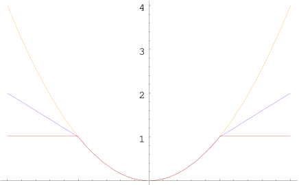
Figure 7.9. A Lévy process has first moment if the Lévy measure integrates $|x|$ for $|x|\geq 1$ (blue line) and second moment if it integrates $x^{2}$ for $|x|\geq 1$ (orange line).

The graphical representation of the functions the Lévy measure must integrate so that a Lévy process has finite moments is given in Figure 7.9. The NIG process possesses moments of all order, while the $\alpha$-stable does not; one can already observe in Figure 7.7 that the tails of the Lévy measure of the $\alpha$-stable are much heavier than the tails of the NIG.

Remark 7.4.

As can be observed from Propositions 7.1, 7.2 and 7.3, the variation of a Lévy process depends on the small jumps (and the Brownian motion), the moment properties depend on the big jumps, while the activity of a Lévy process depends on all the jumps of the process.

8. Some classes of particular interest

We already know that a Brownian motion, a (compound) Poisson process and a Lévy jump-diffusion are Lévy processes, their Lévy-Itô decomposition and their characteristic functions. Here, we present some further subclasses of Lévy processes that are of special interest.

8.1. Subordinator

A subordinator is an a.s. increasing (in $t$) Lévy process. Equivalently, for $L$ to be a subordinator, the triplet must satisfy $\nu(-\infty,0)=0$, $c=0$, $\int_{(0,1)}x\nu(\mathrm{d}x)<\infty$ and $\gamma=b-\int_{(0,1)}x\nu(\mathrm{d}x)>0$.

The Lévy-Itô decomposition of a subordinator is

(8.1) $$L_{t}=\gamma t+\int_{0}^{t}\int_{(0,\infty)}x\mu^{L}(\mathrm{d}s,\mathrm{d}x)$$

and the Lévy-Khintchine formula takes the form

(8.2) $$\mathrm{I\kern-1.99997ptE}[\mathrm{e}^{iuL_{t}}]=\exp\Big{[}t\big{(}iu\gamma+\int_{(0,\infty)}(\mathrm{e}^{iux}-1)\nu(\mathrm{d}x)\big{)}\Big{]}.$$

Two examples of subordinators are the Poisson and the inverse Gaussian process, cf. Figures 8.10 and A.14.

8.2. Jumps of finite variation

A Lévy process has jumps of finite variation if and only if $\int_{|x|\leq 1}|x|\nu(\mathrm{d}x)<\infty$. In this case, the Lévy-Itô decomposition of $L$ resumes the form

(8.3) $$L_{t}=\gamma t+\sqrt{c}W_{t}+\int_{0}^{t}\int_{\mathbb{R}}x\mu^{L}(\mathrm{d}s,\mathrm{d}x)$$

and the Lévy-Khintchine formula takes the form

(8.4) $$\mathrm{I\kern-1.99997ptE}[\mathrm{e}^{iuL_{t}}]=\exp\Big{[}t\big{(}iu\gamma-\frac{u^{2}c}{2}+\int_{\mathbb{R}}(\mathrm{e}^{iux}-1)\nu(\mathrm{d}x)\big{)}\Big{]},$$

where $\gamma$ is defined similarly to subsection 8.1.

Moreover, if $\nu([-1,1])<\infty$, which means that $\nu(\mathbb{R})<\infty$, then the jumps of $L$ correspond to a compound Poisson process.

8.3. Spectrally one-sided

A Lévy processes is called spectrally negative if $\nu(0,\infty)=0$. The Lévy-Itô decomposition of a spectrally negative Lévy process has the form

(8.5) $$L_{t} =bt+\sqrt{c}W_{t}+\int_{0}^{t}\!\int_{x<-1}x\mu^{L}(\mathrm{d}s,\mathrm{d}x)+\int_{0}^{t}\!\!\int_{-1<x<0}\!\!\!\!x(\mu^{L}-\nu^{L})(\mathrm{d}s,\mathrm{d}x)$$

and the Lévy-Khintchine formula takes the form

(8.6) $$\mathrm{I\kern-1.99997ptE}[\mathrm{e}^{iuL_{t}}]=\exp\Big{[}t\big{(}iub-\frac{u^{2}c}{2}+\int_{(-\infty,0)}(\mathrm{e}^{iux}-1-iu1_{\{x>-1\}})\nu(\mathrm{d}x)\Big{]}.$$

Similarly, a Lévy processes is called spectrally positive if $-L$ is spectrally negative.

8.4. Finite first moment

As we have seen already, a Lévy process has finite first moment if and only if $\int_{|x|\geq 1}|x|\nu(\mathrm{d}x)<\infty$. Therefore, we can also compensate the big jumps to form a martingale, hence the Lévy-Itô decomposition of $L$ resumes the form

(8.7) $$L_{t}=b^{\prime}t+\sqrt{c}W_{t}+\int_{0}^{t}\int_{\mathbb{R}}x(\mu^{L}-\nu^{L})(\mathrm{d}s,\mathrm{d}x)$$

and the Lévy-Khintchine formula takes the form

(8.8) $$\mathrm{I\kern-1.99997ptE}[\mathrm{e}^{iuL_{t}}]=\exp\Big{[}t\big{(}iub^{\prime}-\frac{u^{2}c}{2}+\int_{\mathbb{R}}(\mathrm{e}^{iux}-1-iux)\nu(\mathrm{d}x)\big{)}\Big{]},$$

where $b^{\prime}=b+\int_{|x|\geq 1}x\nu(\mathrm{d}x)$.

Remark 8.1 (Assumption ($\mathbb{M}$)).

For the remaining parts we will work only with Lévy process that have finite first moment. We will refer to them as Lévy processes that satisfy Assumption ($\mathbb{M}$). For the sake of simplicity, we suppress the notation $b^{\prime}$ and write $b$ instead.

Figure 8.10. Simulated path of a normal inverse Gaussian (left) and an inverse Gaussian process.

9. Elements from semimartingale theory

A semimartingale is a stochastic process $X=(X_{t})_{0\leq t\leq T}$ which admits the decomposition

(9.1) $$X=X_{0}+M+A$$

where $X_{0}$ is finite and $\mathcal{F}_{0}$-measurable, $M$ is a local martingale with $M_{0}=0$ and $A$ is a finite variation process with $A_{0}=0$. $X$ is a special semimartingale if $A$ is predictable.

Every special semimartingale $X$ admits the following, so-called, canonical decomposition

(9.2) $$X =X_{0}+B+X^{c}+x*(\mu^{X}-\nu^{X}).$$

Here $X^{c}$ is the continuous martingale part of $X$ and $x*(\mu^{X}-\nu^{X})$ is the purely discontinuous martingale part of $X$. $\mu^{X}$ is called the random measure of jumps of $X$; it counts the number of jumps of specific size that occur in a time interval of specific length. $\nu^{X}$ is called the compensator of $\mu^{X}$; for a detailed account, we refer to [Chapter II]JacodShiryaev03.

Remark 9.1.

Note that $W*\mu$, for $W=W(\omega;s,x)$ and the integer-valued measure $\mu=\mu(\omega;\mathrm{d}t,\mathrm{d}x)$, $t\in[0,T]$, $x\in E$, denotes the integral process

$$\int_{0}^{\cdot}\int_{E}W(\omega;t,x)\mu(\omega;\mathrm{d}t,\mathrm{d}x).$$

Consider a predictable function $W:\Omega\times[0,T]\times E\rightarrow\mathbb{R}$ in $G_{\text{loc}}(\mu)$; then $W*(\mu-\nu)$ denotes the stochastic integral

$$\int_{0}^{\cdot}\int_{E}W(\omega;t,x)(\mu-\nu)(\omega;\mathrm{d}t,\mathrm{d}x).$$

Now, recalling the Lévy-Itô decomposition (8.7) and comparing it to (9.2), we can easily deduce that a Lévy process with triplet ($b,c,\nu$) which satisfies Assumption ($\mathbb{M}$), has the following canonical decomposition

(9.3) $$L_{t} =bt+\sqrt{c}W_{t}+\int_{0}^{t}\int_{\mathbb{R}}x(\mu^{L}-\nu^{L})(\mathrm{d}s,\mathrm{d}x),$$

where

$$\int_{0}^{t}\int_{\mathbb{R}}x\mu^{L}(\mathrm{d}s,\mathrm{d}x)=\sum_{0\leq s\leq t}\Delta L_{s}$$

and

$$\mathrm{I\kern-1.99997ptE}\Big{[}\int_{0}^{t}\int_{\mathbb{R}}x\mu^{L}(\mathrm{d}s,\mathrm{d}x)\Big{]}=\int_{0}^{t}\int_{\mathbb{R}}x\nu^{L}(\mathrm{d}s,\mathrm{d}x)=t\int_{\mathbb{R}}x\nu(\mathrm{d}x).$$

Therefore, a Lévy process that satisfies Assumption ($\mathbb{M}$) is a special semimartingale where the continuous martingale part is a Brownian motion with coefficient $\sqrt{c}$ and the random measure of the jumps is a Poisson random measure. The compensator $\nu^{L}$ of the Poisson random measure $\mu^{L}$ is a product measure of the Lévy measure with the Lebesgue measure, i.e. $\nu^{L}=\nu\otimes{\mathchoice{\lambda\mkern-4.5mu{\raisebox{1.72218pt}{\scriptsize$\backslash$}}}{\lambda\mkern-4.83mu{\raisebox{1.72218pt}{\scriptsize$\backslash$}}}{\lambda\mkern-4.5mu{\raisebox{0.86108pt}{\footnotesize$\scriptscriptstyle\backslash$}}}{\lambda\mkern-5.0mu{\raisebox{0.86108pt}{\tiny$\scriptscriptstyle\backslash$}}}}$; one then also writes $\nu^{L}(\mathrm{d}s,\mathrm{d}x)=\nu(\mathrm{d}x)\mathrm{d}s$.

We denote the continuous martingale part of $L$ by $L^{c}$ and the purely discontinuous martingale part of $L$ by $L^{d}$, i.e.

(9.4) $$L_{t}^{c}=\sqrt{c}W_{t} \text{ and }\qquad L_{t}^{d}=\int_{0}^{t}\int_{\mathbb{R}}x(\mu^{L}-\nu^{L})(\mathrm{d}s,\mathrm{d}x).$$

Remark 9.2.

Every Lévy process is also a semimartingale; this follows easily from (9.1) and the Lévy–Itô decomposition of a Lévy process. Every Lévy process with finite first moment (i.e. that satisfies Assumption ($\mathbb{M}$)) is also a special semimartingale; conversely, every Lévy process that is a special semimartingale, has a finite first moment. This is the subject of the next result.

Lemma 9.3.

Let $L$ be a Lévy process with triplet ($b,c,\nu$). The following conditions are equivalent

1. $L$ is a special semimartingale,

2. $\int_{\mathbb{R}}(|x|\wedge|x|^{2})\nu(\mathrm{d}x)<\infty$,

3. $\int_{\mathbb{R}}|x|1_{\{|x|\geq 1\}}\nu(\mathrm{d}x)<\infty$.

Proof.

From Lemma 2.8 in KallsenShiryaev02 we have that, a Lévy process (semimartingale) is special if and only if the compensator of its jump measure satisfies

$$\int_{0}^{\cdot}\int_{\mathbb{R}}(|x|\wedge|x|^{2})\nu^{L}(\mathrm{d}s,\mathrm{d}x)\in\mathcal{V}.$$

For a fixed $t\in\mathbb{R}$, we get

$$\int_{0}^{t}\int_{\mathbb{R}}(|x|\wedge|x|^{2})\nu^{L}(\mathrm{d}s,\mathrm{d}x) =\int_{0}^{t}\int_{\mathbb{R}}(|x|\wedge|x|^{2})\nu(\mathrm{d}x)\mathrm{d}s$$

$$=t\cdot\int_{\mathbb{R}}(|x|\wedge|x|^{2})\nu(\mathrm{d}x)$$

and the last expression is an element of $\mathcal{V}$ if and only if

$$\int_{\mathbb{R}}(|x|\wedge|x|^{2})\nu(\mathrm{d}x)<\infty;$$

this settles $(1)\Leftrightarrow(2)$. The equivalence $(2)\Leftrightarrow(3)$ follows from the properties of the Lévy measure, namely that $\int_{|x|<1}|x|^{2}\nu(\mathrm{d}x)<\infty$, cf. (7.1). ∎

10. Martingales and Lévy processes

We give a condition for a Lévy process to be a martingale and discuss when the exponential of a Lévy process is a martingale.

Proposition 10.1.

Let $L=(L_{t})_{0\leq t\leq T}$ be a Lévy process with Lévy triplet $(b,c,\nu)$ and assume that $\mathrm{I\kern-1.99997ptE}[|L_{t}|]<\infty$, i.e. Assumption $(\mathbb{M})$ holds. $L$ is a martingale if and only if $b=0$. Similarly, $L$ is a submartingale if $b>0$ and a supermartingale if $b<0$.

Proof.

The assertion follows immediately from the decomposition of a Lévy process with finite first moment into a finite variation process, a continuous martingale and a pure-jump martingale, cf. equation (9.3). ∎

Proposition 10.2.

Let $L=(L_{t})_{0\leq t\leq T}$ be a Lévy process with Lévy triplet $(b,c,\nu)$, assume that $\int_{|x|\geq 1}\mathrm{e}^{ux}\nu(\mathrm{d}x)<\infty$, for $u\in\mathbb{R}$ and denote by $\kappa$ the cumulant of $L_{1}$, i.e. $\kappa(u)=\log\mathrm{I\kern-1.99997ptE}[\mathrm{e}^{uL_{1}}]$. The process $M=(M_{t})_{0\leq t\leq T}$, defined via

$$M_{t}=\frac{\mathrm{e}^{uL_{t}}}{\mathrm{e}^{t\kappa(u)}}$$

is a martingale.

Proof.

Applying Proposition 7.3, we get that $\mathrm{I\kern-1.99997ptE}[\mathrm{e}^{uL_{t}}]=\mathrm{e}^{t\kappa(u)}<\infty$, for all ${0\leq t\leq T}$. Now, for $0\leq s\leq t$, we can re-write $M$ as

$$M_{t}=\frac{\mathrm{e}^{uL_{s}}}{\mathrm{e}^{s\kappa(u)}}\frac{\mathrm{e}^{u(L_{t}-L_{s})}}{\mathrm{e}^{(t-s)\kappa(u)}}=M_{s}\frac{\mathrm{e}^{u(L_{t}-L_{s})}}{\mathrm{e}^{(t-s)\kappa(u)}}.$$

Using the fact that a Lévy process has stationary and independent increments, we can conclude

$$\mathrm{I\kern-1.99997ptE}\Big{[}M_{t}\Big{|}\mathcal{F}_{s}\Big{]} =M_{s}\mathrm{I\kern-1.99997ptE}\Big{[}\frac{\mathrm{e}^{u(L_{t}-L_{s})}}{\mathrm{e}^{(t-s)\kappa(u)}}\Big{|}\mathcal{F}_{s}\Big{]}=M_{s}\mathrm{e}^{(t-s)\kappa(u)}\mathrm{e}^{-(t-s)\kappa(u)}$$

$$=M_{s}.\qed$$

The stochastic exponential $\mathcal{E}(L)$ of a Lévy process $L=(L_{t})_{0\leq t\leq T}$ is the solution $Z$ of the stochastic differential equation

(10.1) $$\mathrm{d}Z_{t}=Z_{t-}\mathrm{d}L_{t},\qquad Z_{0}=1,$$

also written as

(10.2) $$Z=1+Z_{-}\cdot L,$$

where $F\cdot Y$ means the stochastic integral $\int_{0}^{\cdot}F_{s}\mathrm{d}Y_{s}$. The stochastic exponential is defined as

(10.3) $$\mathcal{E}(L)_{t}=\exp\left(L_{t}-\frac{1}{2}\langle L^{c}\rangle_{t}\right)\prod_{0\leq s\leq t}\Big{(}1+\Delta L_{s}\Big{)}\mathrm{e}^{-\Delta L_{s}}.$$

Remark 10.3.

The stochastic exponential of a Lévy process that is a martingale is a local martingale (cf. [Theorem I.4.61]JacodShiryaev03) and indeed a (true) martingale when working in a finite time horizon (cf. [Lemma 4.4]Kallsen00).

The converse of the stochastic exponential is the stochastic logarithm, denoted $\mathop{\mathcal{L}\mathrm{og}}X$; for a process $X=(X_{t})_{0\leq t\leq T}$, the stochastic logarithm is the solution of the stochastic differential equation:

(10.4) $$\mathop{\mathcal{L}\mathrm{og}}X_{t}=\int_{0}^{t}\frac{\mathrm{d}X_{s}}{X_{s-}},$$

also written as

(10.5) $$\mathop{\mathcal{L}\mathrm{og}}X=\frac{1}{X_{-}}\cdot X.$$

Now, if $X$ is a positive process with $X_{0}=1$ we have for $\mathop{\mathcal{L}\mathrm{og}}X$

(10.6) $$\mathop{\mathcal{L}\mathrm{og}}X=\log X+\frac{1}{2X^{2}_{-}}\cdot\langle X^{c}\rangle-\sum_{0\leq s\leq\cdot}\bigg{(}\log\Big{(}1+\frac{\Delta X_{s}}{X_{s-}}\Big{)}-\frac{\Delta X_{s}}{X_{s-}}\bigg{)};$$

for more details see KallsenShiryaev02 or Jacod and Shiryaev JacodShiryaev03.

11. Itô’s formula

We state a version of Itô’s formula directly for semimartingales, since this is the natural framework to work into.

Lemma 11.1.

Let $X=(X_{t})_{0\leq t\leq T}$ be a real-valued semimartingale and $f$ a class $C^{2}$ function on $\mathbb{R}$. Then, $f(X)$ is a semimartingale and we have

(11.1) $$f(X_{t}) =f(X_{0})+\int_{0}^{t}f^{\prime}(X_{s-})\mathrm{d}X_{s}+\frac{1}{2}\int_{0}^{t}f^{\prime\prime}(X_{s-})\mathrm{d}\langle X^{c}\rangle_{s}$$

$$\quad+\sum_{0\leq s\leq t}\Big{(}f(X_{s})-f(X_{s-})-f^{\prime}(X_{s-})\Delta X_{s}\Big{)},$$

for all $t\in[0,T]$; alternatively, making use of the random measure of jumps, we have

(11.2) $$f(X_{t}) =f(X_{0})+\int_{0}^{t}f^{\prime}(X_{s-})\mathrm{d}X_{s}+\frac{1}{2}\int_{0}^{t}f^{\prime\prime}(X_{s-})\mathrm{d}\langle X^{c}\rangle_{s}$$

$$\quad+\int_{0}^{t}\int_{\mathbb{R}}\Big{(}f(X_{s-}+x)-f(X_{s-})-f^{\prime}(X_{s-})x\Big{)}\mu^{X}(\mathrm{d}s,\mathrm{d}x).$$

Proof.

See Theorem I.4.57 in JacodShiryaev03. ∎

Remark 11.2.

An interesting account (and proof) of Itô’s formula for Lévy processes of finite variation can be found in [Chapter 4]Kyprianou06.

Lemma 11.3 (Integration by parts).

Let $X,Y$ be semimartingales. Then $XY$ is also a semimartingale and

(11.3) $$XY=\int X_{-}\mathrm{d}Y+\int Y_{-}\mathrm{d}X+[X,Y],$$

where the quadratic covariation of $X$ and $Y$ is given by

(11.4) $$[X,Y]=\langle X^{c},Y^{c}\rangle+\sum_{s\leq\cdot}\Delta X_{s}\Delta Y_{s}.$$

Proof.

See Corollary II.6.2 in Protter04 and Theorem I.4.52 in Jacod and Shiryaev JacodShiryaev03. ∎

As a simple application of Itô’s formula for Lévy processes, we will work out the dynamics of the stochastic logarithm of a Lévy process.

Let $L=(L_{t})_{0\leq t\leq T}$ be a Lévy process with triplet ($b,c,\nu$) and $L_{0}=1$. Consider the $C^{2}$ function $f:\mathbb{R}\rightarrow\mathbb{R}$ with $f(x)=\log|x|$; then, $f^{\prime}(x)=\frac{1}{x}$ and $f^{\prime\prime}(x)=-\frac{1}{x^{2}}$. Applying Itô’s formula to $f(L)=\log|L|$, we get

$$\log|L_{t}| =\log|L_{0}|+\int_{0}^{t}\frac{1}{L_{s-}}\mathrm{d}L_{s}-\frac{1}{2}\int_{0}^{t}\frac{1}{L^{2}_{s-}}\mathrm{d}\langle L^{c}\rangle_{s}$$

$$\qquad+\sum_{0\leq s\leq t}\Big{(}\log|L_{s}|-\log|L_{s-}|-\frac{1}{L_{s-}}\Delta L_{s}\Big{)}$$

$$\Leftrightarrow\mathop{\mathcal{L}\mathrm{og}}L_{t} =\log|L_{t}|+\frac{1}{2}\int_{0}^{t}\frac{\mathrm{d}\langle L^{c}\rangle_{s}}{L^{2}_{s-}}-\sum_{0\leq s\leq t}\Big{(}\log\Big{|}\frac{L_{s}}{L_{s-}}\Big{|}-\frac{\Delta L_{s}}{L_{s-}}\Big{)}.$$

Now, making again use of the random measure of jumps of the process $L$ and using also that $\mathrm{d}\langle L^{c}\rangle_{s}=\mathrm{d}\langle\sqrt{c}W\rangle_{s}=c\mathrm{d}s$, we can conclude that

$$\mathop{\mathcal{L}\mathrm{og}}L_{t} =\log|L_{t}|+\frac{c}{2}\int_{0}^{t}\frac{\mathrm{d}s}{L^{2}_{s-}}-\int_{0}^{t}\int_{\mathbb{R}}\Big{(}\log\Big{|}1+\frac{x}{L_{s-}}\Big{|}-\frac{x}{L_{s-}}\Big{)}\mu^{L}(\mathrm{d}s,\mathrm{d}x).$$

12. Girsanov’s theorem

We will describe a special case of Girsanov’s theorem for semimartingales, where a Lévy process remains a process with independent increments (PII) under the new measure. Here we will restrict ourselves to a finite time horizon, i.e. $T\in[0,\infty)$.

Let $P$ and $\bar{P}$ be probability measures defined on the filtered probability space ($\Omega,\mathcal{F},\mathbf{F}$). Two measures $P$ and $\bar{P}$ are equivalent, if $P(A)=0\Leftrightarrow\bar{P}(A)=0$, for all $A\in\mathcal{F}$, and then one writes $P\sim\bar{P}$.

Given two equivalent measures $P$ and $\bar{P}$, there exists a unique, positive, $P$-martingale $Z=(Z_{t})_{0\leq t\leq T}$ such that $Z_{t}=\mathrm{I\kern-1.99997ptE}\big{[}\frac{\mathrm{d}\bar{P}}{\mathrm{d}P}\big{|}\mathcal{F}_{t}\big{]}$, $\forall\;{0\leq t\leq T}$. $Z$ is called the density process of $\bar{P}$ with respect to $P$.

Conversely, given a measure $P$ and a positive $P$-martingale $Z=(Z_{t})_{0\leq t\leq T}$, one can define a measure $\bar{P}$ on ($\Omega,\mathcal{F},\mathbf{F}$) equivalent to $P$, using the Radon-Nikodym derivative $\mathrm{I\kern-1.99997ptE}\big{[}\frac{\mathrm{d}\bar{P}}{\mathrm{d}P}\big{|}\mathcal{F}_{T}\big{]}=Z_{T}$.

Theorem 12.1.

Let $L=(L_{t})_{0\leq t\leq T}$ be a Lévy process with triplet $(b,c,\nu)$ under $P$, that satisfies Assumption $(\mathbb{M})$, cf. Remark 8.1. Then, $L$ has the canonical decomposition

(12.1) $$L_{t}=bt+\sqrt{c}W_{t}+\int_{0}^{t}\int_{\mathbb{R}}x(\mu^{L}-\nu^{L})(\mathrm{d}s,\mathrm{d}x).$$

1. Assume that $P\sim\bar{P}$ with density process $Z$. Then, there exist a deterministic process $\beta$ and a measurable non-negative deterministic process $Y$, satisfying

   (12.2) $$\int_{0}^{t}\int_{\mathbb{R}}|x\big{(}Y(s,x)-1\big{)}|\nu(\mathrm{d}x)\mathrm{d}s<\infty,$$

   and

   $$\int_{0}^{t}\big{(}c\cdot\beta^{2}_{s}\big{)}\mathrm{d}s<\infty,$$

   $\bar{P}$-a.s. for ${0\leq t\leq T}$; they are defined by the following formulae:

   (12.3) $$\langle Z^{c},L^{c}\rangle=\int_{0}^{\cdot}(c\cdot\beta_{s}\cdot Z_{s-})\mathrm{d}s$$

   and

   (12.4) $$Y=M_{\mu^{L}}^{P}\left(\frac{Z}{Z_{-}}\Big{|}\widetilde{\mathcal{P}}\right).$$

1. Conversely, if $Z$ is a positive martingale of the form

   (12.5) $$Z =\exp\Big{[}\int_{0}^{\cdot}\beta_{s}\sqrt{c}\mathrm{d}W_{s}-\frac{1}{2}\int_{0}^{\cdot}\beta^{2}_{s}c\mathrm{d}s$$

   $$\qquad\qquad+\int_{0}^{\cdot}\int_{\mathbb{R}}(Y(s,x)-1)(\mu^{L}-\nu^{L})(\mathrm{d}s,\mathrm{d}x)$$

   $$\qquad\qquad-\int_{0}^{\cdot}\int_{\mathbb{R}}(Y(s,x)-1-\ln(Y(s,x)))\mu^{L}(\mathrm{d}s,\mathrm{d}x)\Big{]}.$$

   then it defines a probability measure $\bar{P}$ on $(\Omega,\mathcal{F},\mathbf{F})$, such that $P\sim\bar{P}$.

1. In both cases, we have that $\bar{W}=W-\int_{0}^{\cdot}\sqrt{c}\beta_{s}\mathrm{d}s$ is a $\bar{P}$-Brownian motion, $\bar{\nu}^{L}(\mathrm{d}s,\mathrm{d}x)=Y(s,x)\nu^{L}(\mathrm{d}s,\mathrm{d}x)$ is the $\bar{P}$-compensator of $\mu^{L}$ and $L$ has the following canonical decomposition under $\bar{P}$:

   (12.6) $$L_{t}=\bar{b}t+\sqrt{c}\bar{W}_{t}+\int_{0}^{t}\int_{\mathbb{R}}x(\mu^{L}-\bar{\nu}^{L})(\mathrm{d}s,\mathrm{d}x),$$

   where

   (12.7) $$\bar{b}t=bt+\int_{0}^{t}c\beta_{s}\mathrm{d}s+\int_{0}^{t}\int_{\mathbb{R}}x\big{(}Y(s,x)-1\big{)}\nu^{L}(\mathrm{d}s,\mathrm{d}x).$$

Proof.

Theorems III.3.24, III.5.19 and III.5.35 in JacodShiryaev03 yield the result. ∎

Remark 12.2.

In (12.4) $\widetilde{\mathcal{P}}={\mathcal{P}}\otimes\mathcal{B}(\mathbb{R})$ is the $\sigma$-field of predictable sets in $\widetilde{\Omega}=\Omega\times[0,T]\times\mathbb{R}$ and $M_{\mu^{L}}^{P}=\mu^{L}(\omega;\mathrm{d}t,\mathrm{d}x)P(\mathrm{d}\omega)$ is the positive measure on $(\Omega\times[0,T]\times\mathbb{R},\mathcal{F}\otimes\mathcal{B}([0,T])\otimes\mathcal{B}(\mathbb{R}))$ defined by

(12.8) $$M_{\mu^{L}}^{P}(W)=E(W*\mu^{L})_{T},$$

for measurable nonnegative functions $W=W(\omega;t,x)$ given on $\Omega\times[0,T]\times\mathbb{R}$. Now, the conditional expectation $M_{\mu^{L}}^{P}\Big{(}\frac{\textstyle Z}{\textstyle Z_{-}}|\widetilde{\mathcal{P}}\Big{)}$ is, by definition, the $M_{\mu^{L}}^{P}$-a.s. unique $\widetilde{\mathcal{P}}$-measurable function $Y$ with the property

(12.9) $$M_{\mu^{L}}^{P}\Big{(}\frac{Z}{Z_{-}}U\Big{)}=M_{\mu^{L}}^{P}(YU),$$

for all nonnegative $\widetilde{\mathcal{P}}$-measurable functions $U=U(\omega;t,x)$.

Remark 12.3.

Notice that from condition (12.2) and assumption ($\mathbb{M}$), follows that $L$ has finite first moment under $\bar{P}$ as well, i.e.

(12.10) $$\bar{\mathrm{I\kern-1.99997ptE}}|L_{t}|<\infty,\;\;\;\text{ for all }\;{0\leq t\leq T}.$$

Verification follows from Proposition 7.3 and direct calculations.

Remark 12.4.

In general, $L$ is not necessarily a Lévy process under the measure $\bar{P}$; this depends on the tuple ($\beta,Y$). The following cases exist.

(G1):

if ($\beta,Y$) are deterministic and independent of time, then $L$ remains a Lévy process under $\bar{P}$; its triplet is ($\bar{b},c,Y\cdot\nu$).

(G2):

if ($\beta,Y$) are deterministic but depend on time, then $L$ becomes a process with independent (but not stationary) increments under $\bar{P}$, often called an additive process.

(G3):

if ($\beta,Y$) are neither deterministic nor independent of time, then we just know that $L$ is a semimartingale under $\bar{P}$.

Remark 12.5.

Notice that $c$, the diffusion coefficient, and $\mu^{L}$, the random measure of jumps of $L$, did not change under the change of measure from $P$ to $\bar{P}$. That happens because $c$ and $\mu^{L}$ are path properties of the process and do not change under an equivalent change of measure. Intuitively speaking, the paths do not change, the probability of certain paths occurring changes.

Example 12.6.

Assume that $L$ is a Lévy process with canonical decomposition (12.1) under $P$. Assume that $P\sim\bar{P}$ and the density process is

(12.11) $$Z_{t} =\exp\Big{[}\beta\sqrt{c}W_{t}+\int_{0}^{t}\int_{\mathbb{R}}\alpha x(\mu^{L}-\nu^{L})(\mathrm{d}s,\mathrm{d}x)$$

$$\qquad\qquad-\Big{(}\frac{c\beta^{2}}{2}+\int_{\mathbb{R}}(\mathrm{e}^{\alpha x}-1-\alpha x)\nu(\mathrm{d}x)\Big{)}t\Big{]},$$

where $\beta\in\mathbb{R}_{\geqslant 0}$ and $\alpha\in\mathbb{R}$ are constants.

Then, comparing (12.11) with (12.5), we have that the tuple of functions that characterize the change of measure is ($\beta,Y)=(\beta,f$), where $f(x)=\mathrm{e}^{\alpha x}$. Because $(\beta,f)$ are deterministic and independent of time, $L$ remains a Lévy process under $\bar{P}$, its Lévy triplet is ($\bar{b},c,f\nu$) and its canonical decomposition is given by equations (12.6) and (12.7).

Actually, the change of measure of the previous example corresponds to the so-called Esscher transformation or exponential tilting. In chapter 3 of Kyprianou06, one can find a significantly easier proof of Girsanov’s theorem for Lévy processes for the special case of the Esscher transform. Here, we reformulate the result of example 12.6 and give a complete proof (inspired by EberleinPapapantoleon05b).

Proposition 12.7.

Let $L=(L_{t})_{0\leq t\leq T}$ be a Lévy process with canonical decomposition (12.1) under $P$ and assume that $\mathrm{I\kern-1.99997ptE}[\mathrm{e}^{uL_{t}}]<\infty$ for all $u\in[-p,p]$, $p>0$. Assume that $P\sim\bar{P}$ with density process $Z=(Z_{t})_{0\leq t\leq T}$, or conversely, assume that $\bar{P}$ is defined via the Radon-Nikodym derivative $\frac{\mathrm{d}\bar{P}}{\mathrm{d}P}=Z_{T}$; here, we have that

(12.12) $$Z_{t} =\frac{\mathrm{e}^{\beta L_{t}^{c}}\mathrm{e}^{\alpha L_{t}^{d}}}{\mathrm{I\kern-1.99997ptE}[\mathrm{e}^{\beta L_{t}^{c}}]\mathrm{I\kern-1.99997ptE}[\mathrm{e}^{\alpha L_{t}^{d}}]}$$

for $\beta\in\mathbb{R}$ and $|\alpha|<p$. Then, $L$ remains a Lévy process under $\bar{P}$, its Lévy triplet is ($\bar{b},c,\bar{\nu}$), where $\bar{\nu}=f\cdot\nu$ for $f(x)=\mathrm{e}^{\alpha x}$, and its canonical decomposition is given by the following equations

(12.13) $$L_{t}=\bar{b}t+\sqrt{c}\bar{W}_{t}+\int_{0}^{t}\int_{\mathbb{R}}x(\mu^{L}-\bar{\nu}^{L})(\mathrm{d}s,\mathrm{d}x),$$

and

(12.14) $$\bar{b}=b+\beta c+\int_{\mathbb{R}}x\big{(}\mathrm{e}^{\alpha x}-1\big{)}\nu(\mathrm{d}x).$$

Proof.

Firstly, using Proposition 10.2, we can immediately deduce that $Z$ is a positive $P$-martingale; moreover, $Z_{0}=1$. Hence, $Z$ serves as a density process.

Secondly, we will show that $L$ has independent and stationary increments under $\bar{P}$. Using that $L$ has independent and stationary increments under $P$ and that $Z$ is a $P$-martingale, we arrive at the following helpful conclusions: for any $B\in\mathcal{B}(\mathbb{R})$, $F_{s}\in\mathcal{F}_{s}$ and $0\leq s<t\leq T$

1. $1_{\{L_{t}-L_{s}\in B\}}\frac{Z_{t}}{Z_{s}}$ is independent of $1_{\{F_{s}\}}Z_{s}$ and of $Z_{s}$;

2. $E[Z_{s}]=1$.

Then, we have that

$$\bar{P}(\{L_{t}-L_{s}\in B\}\cap F_{s}) =\mathrm{I\kern-1.99997ptE}\Big{[}1_{\{L_{t}-L_{s}\in B\}}1_{\{F_{s}\}}Z_{t}\Big{]}$$

$$=\mathrm{I\kern-1.99997ptE}\Big{[}1_{\{L_{t}-L_{s}\in B\}}\frac{Z_{t}}{Z_{s}}\Big{]}\mathrm{I\kern-1.99997ptE}\big{[}1_{\{F_{s}\}}Z_{s}\big{]}$$

$$=\mathrm{I\kern-1.99997ptE}\Big{[}1_{\{L_{t}-L_{s}\in B\}}\frac{Z_{t}}{Z_{s}}\Big{]}\mathrm{I\kern-1.99997ptE}[Z_{s}]\mathrm{I\kern-1.99997ptE}\big{[}1_{\{F_{s}\}}Z_{s}\big{]}$$

$$=\mathrm{I\kern-1.99997ptE}\Big{[}1_{\{L_{t}-L_{s}\in B\}}Z_{t}\Big{]}\mathrm{I\kern-1.99997ptE}\big{[}1_{\{F_{s}\}}Z_{s}\big{]}$$

$$=\bar{P}(\{L_{t}-L_{s}\in B\})\bar{P}(F_{s})$$

which yields the independence of the increments. Similarly, regarding the stationarity of the increments of $L$ under $\bar{P}$, we have that

$$\bar{P}(\{L_{t}-L_{s}\in B\}) =\mathrm{I\kern-1.99997ptE}\big{[}1_{\{L_{t}-L_{s}\in B\}}Z_{t}\big{]}$$

$$=\mathrm{I\kern-1.99997ptE}\big{[}1_{\{L_{t}-L_{s}\in B\}}\frac{Z_{t}}{Z_{s}}\big{]}\mathrm{I\kern-1.99997ptE}\big{[}Z_{s}\big{]}$$

$$=\mathrm{I\kern-1.99997ptE}\Big{[}1_{\{L_{t}-L_{s}\in B\}}\frac{\mathrm{e}^{\alpha(L_{t}^{c}-L_{s}^{c})}\mathrm{e}^{\beta(L_{t}^{d}-L_{s}^{d})}}{\mathrm{I\kern-1.99997ptE}[\mathrm{e}^{\alpha(L_{t}^{c}-L_{s}^{c})}\mathrm{e}^{\beta(L_{t}^{d}-L_{s}^{d})}]}\Big{]}$$

$$=\mathrm{I\kern-1.99997ptE}\Big{[}1_{\{L_{t}-L_{s}\in B\}}\frac{\mathrm{e}^{\alpha L_{t-s}^{c}+\beta L_{t-s}^{d}}}{\mathrm{I\kern-1.99997ptE}[\mathrm{e}^{\alpha L_{t-s}^{c}+\beta L_{t-s}^{d}}]}\Big{]}$$

$$=\mathrm{I\kern-1.99997ptE}\big{[}1_{\{L_{t-s}\in B\}}Z_{t-s}\big{]}$$

$$=\bar{P}(\{L_{t-s}\in B\})$$

which yields the stationarity of the increments.

Thirdly, we determine the characteristic function of $L$ under $\bar{P}$, which also yields the triplet and canonical decomposition. Applying Theorem 25.17 in Sato99, the moment generating function $M_{L_{t}}$ of $L_{t}$ exists for $u\in\mathbb{C}$ with $\Re u\in[-p,p]$. We get

$$\bar{\mathrm{I\kern-1.99997ptE}}\big{[}\mathrm{e}^{zL_{t}}\big{]} =\mathrm{I\kern-1.99997ptE}\big{[}\mathrm{e}^{zL_{t}}Z_{t}\big{]}=\mathrm{I\kern-1.99997ptE}\bigg{[}\frac{\mathrm{e}^{zL_{t}}\mathrm{e}^{\beta L_{t}^{c}}\mathrm{e}^{\alpha L_{t}^{d}}}{\mathrm{I\kern-1.99997ptE}[\mathrm{e}^{\beta L_{t}^{c}}]\mathrm{I\kern-1.99997ptE}[\mathrm{e}^{\alpha L_{t}^{d}}]}\bigg{]}=\frac{\mathrm{I\kern-1.99997ptE}[\mathrm{e}^{zbt}\mathrm{e}^{(z+\beta)L_{t}^{c}}\mathrm{e}^{(z+\alpha)L_{t}^{d}}]}{\mathrm{I\kern-1.99997ptE}[\mathrm{e}^{\beta L_{t}^{c}}]\mathrm{I\kern-1.99997ptE}[\mathrm{e}^{\alpha L_{t}^{d}}]}$$

$$=\exp\left(t\Big{[}zb+\frac{(z+\beta)^{2}c}{2}+\int_{\mathbb{R}}\big{(}\mathrm{e}^{(z+\alpha)x}-1-(z+\alpha)x\big{)}\nu(\mathrm{d}x)\right.$$

$$\qquad\qquad\left.-\frac{\beta^{2}c}{2}-\int_{\mathbb{R}}\big{(}\mathrm{e}^{\alpha x}-1-\alpha x\big{)}\nu(\mathrm{d}x)\Big{]}\right)$$

$$=\exp\left(t\Big{[}z\big{(}b+\beta c+\int_{\mathbb{R}}x\big{(}\mathrm{e}^{\alpha x}-1\big{)}\nu(\mathrm{d}x)\big{)}+\frac{z^{2}c}{2}\right.$$

$$\qquad\qquad\left.+\int_{\mathbb{R}}\big{(}\mathrm{e}^{zx}-1-zx\big{)}\mathrm{e}^{\alpha x}\nu(\mathrm{d}x)\Big{]}\right)$$

$$=\exp\left(t\Big{[}z\bar{b}+\frac{z^{2}c}{2}+\int_{\mathbb{R}}\big{(}\mathrm{e}^{zx}-1-zx\big{)}\bar{\nu}(\mathrm{d}x)\Big{]}\right).$$

Finally, the statement follows by proving that $\bar{\nu}(\mathrm{d}x)=\mathrm{e}^{\alpha x}\nu(\mathrm{d}x)$ is a Lévy measure, i.e. $\int_{\mathbb{R}}(1\wedge x^{2})\mathrm{e}^{\alpha x}\nu(\mathrm{d}x)<\infty$. It suffices to note that

(12.15) $$\int_{|x|\leq 1}x^{2}\mathrm{e}^{\alpha x}\nu(\mathrm{d}x)\leq C\int_{|x|\leq 1}x^{2}\nu(\mathrm{d}x)<\infty,$$

where $C$ is a positive constant, because $\nu$ is a Lévy measure; the other part follows from the assumptions, since $|\alpha|<p$. ∎

Remark 12.8.

Girsanov’s theorem is a very powerful tool, widely used in mathematical finance. In the second part, it will provide the link between the ‘real-world’ and the ‘risk-neutral’ measure in a Lévy-driven asset price model. Other applications of Girsanov’s theorem allow to simplify certain valuation problems, cf. e.g. Papapantoleon06 and references therein.

13. Construction of Lévy processes

Three popular methods to construct a Lévy process are described below.

(C1):

Specifying a Lévy triplet; more specifically, whether there exists a Brownian component or not and what is the Lévy measure. Examples of Lévy process constructed this way include the standard Brownian motion, which has Lévy triplet $(0,1,0)$ and the Lévy jump-diffusion, which has Lévy triplet $(b,\sigma^{2},\lambda F)$.

(C2):

Specifying an infinitely divisible random variable as the density of the increments at time scale 1 (i.e. $L_{1}$). Examples of Lévy process constructed this way include the standard Brownian motion, where $L_{1}\sim\text{Normal}(0,1)$ and the normal inverse Gaussian process, where $L_{1}\sim\text{NIG}(\alpha,\beta,\delta,\mu)$.

(C3):

Time-changing Brownian motion with an independent increasing Lévy process. Let $W$ denote the standard Brownian motion; we can construct a Lévy process by ‘replacing’ the (calendar) time $t$ by an independent increasing Lévy process $\tau$, therefore $L_{t}:=W_{\tau(t)}$, ${0\leq t\leq T}$. The process $\tau$ has the useful – in Finance – interpretation as ‘business time’. Models constructed this way include the normal inverse Gaussian process, where Brownian motion is time-changed with the inverse Gaussian process and the variance gamma process, where Brownian motion is time-changed with the gamma process.

Naturally, some processes can be constructed using more than one methods. Nevertheless, each method has some distinctive advantages which are very useful in applications. The advantages of specifying a triplet (C1) are that the characteristic function and the pathwise properties are known and allows the construction of a rich variety of models; the drawbacks are that parameter estimation and simulation (in the infinite activity case) can be quite involved. The second method (C2) allows the easy estimation and simulation of the process; on the contrary the structure of the paths might be unknown. The method of time-changes (C3) allows for easy simulation, yet estimation might be quite difficult.

14. Simulation of Lévy processes

We shall briefly describe simulation methods for Lévy processes. Our attention is focused on finite activity Lévy processes (i.e. Lévy jump-diffusions) and some special cases of infinite activity Lévy processes, namely the normal inverse Gaussian and the variance gamma processes. Several speed-up methods for the Monte Carlo simulation of Lévy processes are presented in Webber05.

Here, we do not discuss simulation methods for random variables with known density; various algorithms can be found in Devroye86, also available online at http://cg.scs.carleton.ca/ luc/rnbookindex.html.

14.1. Finite activity

Assume we want to simulate the Lévy jump-diffusion

$$L_{t}=bt+\sigma W_{t}+\sum_{k=1}^{N_{t}}J_{k}$$

where $N_{t}\sim\text{Poisson}(\lambda t)$ and $J\sim F(\mathrm{d}x)$. $W$ denotes a standard Brownian motion, i.e. $W_{t}\sim\text{Normal}(0,t)$.

We can simulate a discretized trajectory of the Lévy jump-diffusion $L$ at fixed time points $t_{1},\ldots,t_{n}$ as follows:

• generate a standard normal variate and transform it into a normal variate, denoted $G_{i}$, with variance $\sigma\Delta t_{i}$, where $\Delta t_{i}=t_{i}-t_{i-1}$;

• generate a Poisson random variate $N$ with parameter $\lambda T$;

• generate $N$ random variates $\tau_{k}$ uniformly distributed in $[0,T]$; these variates correspond to the jump times;

• simulate the law of jump size $J$, i.e. simulate random variates $J_{k}$ with law $F(\mathrm{d}x)$.

The discretized trajectory is

$$L_{t_{i}}=bt_{i}+\sum_{j=1}^{i}G_{j}+\sum_{k=1}^{N}1_{\{\tau_{k}<t_{i}\}}J_{k}.$$

14.2. Infinite activity

The variance gamma and the normal inverse Gaussian process can be easily simulated because they are time-changed Brownian motions; we follow ContTankov03 closely. A general treatment of simulation methods for infinite activity Lévy processes can be found in ContTankov03 and Schoutens03.

Assume we want to simulate a normal inverse Gaussian (NIG) process with parameters $\alpha,\beta,\delta,\mu$; cf. also section 16.5. We can simulate a discretized trajectory at fixed time points $t_{1},\ldots,t_{n}$ as follows:

• simulate $n$ independent inverse Gaussian variables $I_{i}$ with parameters $(\delta\Delta t_{i})^{2}$ and $\alpha^{2}-\beta^{2}$, where $\Delta t_{i}=t_{i}-t_{i-1}$, $i=1,\ldots,n$;

• simulate $n$ i.i.d. standard normal variables $G_{i}$;

• set $\Delta L_{i}=\mu\Delta t_{i}+\beta I_{i}+\sqrt{I_{i}}G_{i}$.

The discretized trajectory is

$$L_{t_{i}}=\sum_{k=1}^{i}\Delta L_{k}.$$

Assume we want to simulate a variance gamma (VG) process with parameters $\sigma,\theta,\kappa$; we can simulate a discretized trajectory at fixed time points $t_{1},\ldots,t_{n}$ as follows:

• simulate $n$ independent gamma variables $\Gamma_{i}$ with parameter $\frac{\Delta t_{i}}{\kappa}$

• set $\Gamma_{i}=\kappa\Gamma_{i}$;

• simulate $n$ standard normal variables $G_{i}$;

• set $\Delta L_{i}=\theta\Gamma_{i}+\sigma\sqrt{\Gamma_{i}}G_{i}$.

The discretized trajectory is

$$L_{t_{i}}=\sum_{k=1}^{i}\Delta L_{k}.$$

Part II Applications in Finance

15. Asset price model

We describe an asset price model driven by a Lévy process, both under the ‘real’ and under the ‘risk-neutral’ measure. Then, we present an informal account of market incompleteness.

15.1. Real-world measure

Under the real-world measure, we model the asset price process as the exponential of a Lévy process, that is

(15.1) $$S_{t}=S_{0}\exp L_{t},\quad{0\leq t\leq T},$$

where, $L$ is the Lévy process whose infinitely divisible distribution has been estimated from the data set available for the particular asset. Hence, the log-returns of the model have independent and stationary increments, which are distributed – along time intervals of specific length, e.g. 1 – according to an infinitely divisible distribution $\mathcal{L}(X)$, i.e. $L_{1}\stackrel{{\scriptstyle\mathrm{d}}}{{=}}X$.

Naturally, the path properties of the process $L$ carry over to $S$; if, for example, $L$ is a pure-jump Lévy process, then $S$ is also a pure-jump process. This fact allows us to capture, up to a certain extent, the microstructure of price fluctuations, even on an intraday time scale.

An application of Itô’s formula yields that $S=(S_{t})_{0\leq t\leq T}$ is the solution of the stochastic differential equation

(15.2) $$\mathrm{d}S_{t}=S_{t-}\Big{(}\mathrm{d}L_{t}+\frac{c}{2}\mathrm{d}t+\int_{\mathbb{R}}(\mathrm{e}^{x}-1-x)\mu^{L}(\mathrm{d}t,\mathrm{d}x)\Big{)}.$$

We could also specify $S$ by replacing the Brownian motion in the Black–Scholes SDE by a Lévy process, i.e. via

(15.3) $$\mathrm{d}S_{t}=S_{t^{-}}\mathrm{d}L_{t},$$

whose solution is the stochastic exponential

(15.4) $$S_{t}=S_{0}\mathcal{E}(L_{t}).$$

The second approach is unfavorable for financial applications, because ($a$) the asset price can take negative values, unless jumps are restricted to be larger than $-1$, i.e. $\text{supp}(\nu)\subset[-1,\infty)$, and ($b$) the distribution of log-returns is not known. Of course, in the special case of the Black–Scholes model the two approaches coincide.

Remark 15.1.

The two modeling approaches are nevertheless closely related and, in some sense, complementary of each other. One approach is suitable for studying the distributional properties of the price process and the other for investigating the martingale properties. For the connection between the natural and stochastic exponential for Lévy processes, we refer to Lemma A.8 in GollKallsen00.

The fact that the price process is driven by a Lévy process, makes the market, in general, incomplete; the only exceptions are the markets driven by the Normal (Black-Scholes model) and Poisson distributions. Therefore, there exists a large set of equivalent martingale measures, i.e. candidate measures for risk-neutral valuation.

EberleinJacod97 provide a thorough analysis and characterization of the set of equivalent martingale measures for Lévy-driven models. Moreover, they prove that the range of option prices for a convex payoff function, e.g. a call option, under all possible equivalent martingale measures spans the whole no-arbitrage interval, e.g. $[(S_{0}-K\mathrm{e}^{-rT})^{+},S_{0}]$ for a European call option with strike $K$. Selivanov05 discusses the existence and uniqueness of martingale measures for exponential Lévy models in finite and infinite time horizon and for various specifications of the no-arbitrage condition.

The Lévy market can be completed using particular assets, such as moment derivatives (e.g. variance swaps), and then there exists a unique equivalent martingale measure; see Corcuera, Nualart, and Schoutens CorcueraNualartSchoutens05,CorcueraNualartSchoutens05b. For example, if an asset is driven by a Lévy jump-diffusion

(15.5) $$L_{t}=bt+\sqrt{c}W_{t}+\sum_{k=1}^{N_{t}}J_{k}$$

where $J_{k}\equiv\alpha$ $\forall k$, then the market can be completed using only variance swaps on this asset; this example will be revisited in section 15.3.

15.2. Risk-neutral measure

Under the risk neutral measure, denoted by $\bar{P}$, we model the asset price process as an exponential Lévy process

(15.6) $$S_{t}=S_{0}\exp L_{t}$$

where the Lévy process $L$ has the triplet $(\bar{b},\bar{c},\bar{\nu})$ and satisfies Assumptions ($\mathbb{M}$) (cf. Remark 8.1) and ($\mathbb{EM}$) (see below).

The process $L$ has the canonical decomposition

(15.7) $$L_{t}=\bar{b}t+\sqrt{\bar{c}}\bar{W}_{t}+\int_{0}^{t}\int_{\mathbb{R}}x(\mu^{L}-\bar{\nu}^{L})(\mathrm{d}s,\mathrm{d}x)$$

where $\bar{W}$ is a $\bar{P}$-Brownian motion and $\bar{\nu}^{L}$ is the $\bar{P}$-compensator of the jump measure $\mu^{L}$.

Because we have assumed that $\bar{P}$ is a risk neutral measure, the asset price has mean rate of return $\mu\triangleq r-\delta$ and the discounted and re-invested process $(\mathrm{e}^{(r-\delta)t}S_{t})_{0\leq t\leq T}$, is a martingale under $\bar{P}$. Here $r\geq 0$ is the (domestic) risk-free interest rate, $\delta\geq 0$ the continuous dividend yield (or foreign interest rate) of the asset. Therefore, the drift term $\bar{b}$ takes the form

(15.8) $$\bar{b}=r-\delta-\frac{\bar{c}}{2}-\int_{\mathbb{R}}(\mathrm{e}^{x}-1-x)\bar{\nu}(\mathrm{d}x);$$

see EberleinPapapantoleonShiryaev06 and Papapantoleon06 for all the details.

Assumption ($\mathbb{EM}$).

We assume that the Lévy process $L$ has finite first exponential moment, i.e.

(15.9) $$\bar{\mathrm{I\kern-1.99997ptE}}[\mathrm{e}^{L_{t}}]<\infty.$$

There are various ways to choose the martingale measure such that it is equivalent to the real-world measure. We refer to GollRueschendorf01 for a unified exposition – in terms of $f$-divergences – of the different methods for selecting an equivalent martingale measure (EMM). Note that, some of the proposed methods to choose an EMM preserve the Lévy property of log-returns; examples are the Esscher transformation and the minimal entropy martingale measure (cf. EscheSchweizer05).

The market practice is to consider the choice of the martingale measure as the result of a calibration to market data of vanilla options. Hakala and Wystup HakalaWystup02b describe the calibration procedure in detail. ContTankov04 ContTankov04,ContTankov05 and BelomestnyReiss05 present numerically stable calibration methods for Lévy driven models.

15.3. On market incompleteness

In order to gain a better understanding of why the market is incomplete, let us make the following observation. Assume that the price process of a financial asset is modeled as an exponential Lévy process under both the real and the risk-neutral measure. Assume that these measures, denoted $P$ and $\bar{P}$, are equivalent and denote the triplet of the Lévy process under $P$ and $\bar{P}$ by $(b,c,\nu)$ and $(\bar{b},\bar{c},\bar{\nu})$ respectively.

Now, applying Girsanov’s theorem we get that these triplets are related via $\bar{c}=c$, $\bar{\nu}=Y\cdot\nu$ and

(15.10) $$\bar{b}=b+c\beta+x(Y-1)*\nu,$$

where $(\beta,Y)$ is the tuple of functions related to the density process. On the other hand, from the martingale condition we get that

(15.11) $$\bar{b}=r-\frac{\bar{c}}{2}-(\mathrm{e}^{x}-1-x)*\bar{\nu}.$$

Equating (15.10) and (15.11) and using $c=\bar{c}$ and $\nu=Y\cdot\bar{\nu}$, we have that

$$0 =b+c\beta+x(Y-1)*\nu-r+\frac{\bar{c}}{2}+(\mathrm{e}^{x}-1-x)*\bar{\nu}$$

(15.12) $$\Leftrightarrow 0 =b-r+c(\beta+\frac{1}{2})+\big{(}(\mathrm{e}^{x}-1)Y-x\big{)}*\nu;$$

therefore, we have one equation but two unknown parameters, $\beta$ and $Y$ stemming from the change of measure. Every solution tuple $(\beta,Y)$ of equation (15.3) corresponds to a different equivalent martingale measure, which explains why the market is not complete. The tuple $(\beta,Y)$ could also be termed the tuple of ‘market price of risk’.

Example 15.2 (Black–Scholes model).

Let us consider the Black–Scholes model, where the driving process is a Brownian motion with drift, i.e. $L_{t}=bt+\sqrt{c}W_{t}$. Then, equation (15.3) has a unique solution, namely

(15.13) $$\beta=\frac{r-b}{c}-\frac{1}{2},$$

the martingale measure is unique and the market is complete. We can also easily check that plugging (15.13) into (15.10), we recover the martingale condition (15.11).

Remark 15.3.

The quantity $\beta$ in (15.13) is nothing else than the so-called market price of risk. The difference from the quantity often encountered in textbooks, i.e. $\frac{r-\mu}{c}$, stems from the fact that we model using the natural instead of the stochastic exponential, i.e. using SDE (15.2) and not (15.3).

Example 15.4 (Poisson model).

Let us consider the Poisson model, where the driving motion is a Poisson process with intensity $\lambda>0$ and jump size $\alpha$, i.e. $L_{t}=bt+\alpha N_{t}$ and $\nu(\mathrm{d}x)=\lambda 1_{\{\alpha\}}(\mathrm{d}x)$. Then, equation (15.3) has a unique solution for $Y$, which is

$$0 =b-r+\big{(}(\mathrm{e}^{x}-1)Y-x\big{)}*\lambda 1_{\{\alpha\}}(\mathrm{d}x)$$

$$\Leftrightarrow 0 =b-r+\big{(}(\mathrm{e}^{\alpha}-1)Y-\alpha\big{)}\lambda$$

(15.14) $$\Leftrightarrow Y =\frac{r-b+\alpha\lambda}{(\mathrm{e}^{\alpha}-1)\lambda};$$

therefore the martingale measure is unique and the market is complete. By the analogy to the Black–Scholes case, we could call the quantity $Y$ in (15.4) the market price of jump risk.

Moreover, we can also check that plugging (15.4) into (15.10), we recover the martingale condition (15.11); indeed, we have that

$$\bar{b} =b+\alpha\lambda(Y-1)$$

$$=b+\alpha\lambda(Y-1)+(\mathrm{e}^{\alpha}-1)Y\lambda-(\mathrm{e}^{\alpha}-1)Y\lambda$$

$$=r-(\mathrm{e}^{\alpha}-1-\alpha)\bar{\lambda},$$

where we have used (15.4) and that $\bar{\nu}=Y\cdot\nu$, which in the current framework translates to $\bar{\lambda}=Y\lambda$.

Example 15.5 (A simple incomplete model).

Assume that the driving process consists of a drift, a Brownian motion and a Poisson process, i.e. $L_{t}=bt+\sqrt{c}W_{t}+\alpha N_{t}$, as in examples 15.2 and 15.4. Based on (15.13) and (15.4) we postulate that the solutions of equation (15.3) are of the form

(15.15) $$\beta_{\varepsilon}=\varepsilon\frac{r-b}{c}-\frac{1}{2}\quad\text{ and }\quad Y_{\varepsilon}=\frac{(1-\varepsilon)(r-b)+\alpha\lambda}{(\mathrm{e}^{\alpha}-1)\lambda}$$

for any $\varepsilon\in(0,1)$. One can easily verify that $\beta_{\varepsilon}$ and $Y_{\varepsilon}$ satisfy (15.3). But then, to any $\varepsilon\in(0,1)$ corresponds an equivalent martingale measure and we can easily conclude that this simple market is incomplete.

16. Popular models

In this section, we review some popular models in the mathematical finance literature from the point of view of Lévy processes. We describe their Lévy triplets and characteristic functions and provide, whenever possible, their – infinitely divisible – laws.

16.1. Black–Scholes

The most famous asset price model based on a Lévy process is that of Samuelson65, BlackScholes73 and Merton Merton73. The log-returns are normally distributed with mean $\mu$ and variance $\sigma^{2}$, i.e. $L_{1}\sim\text{Normal}(\mu,\sigma^{2})$ and the density is

$$f_{L_{1}}(x)=\frac{1}{\sigma\sqrt{2\pi}}\exp\Big{[}-\frac{(x-\mu)^{2}}{2\sigma^{2}}\Big{]}.$$

The characteristic function is

$$\varphi_{L_{1}}(u)=\exp\Big{[}i\mu u-\frac{\sigma^{2}u^{2}}{2}\Big{]},$$

the first and second moments are

$$\text{E}[L_{1}]=\mu, \qquad\text{Var}[L_{1}]=\sigma^{2},$$

while the skewness and kurtosis are

$$\text{skew}[L_{1}]=0, \qquad\text{kurt}[L_{1}]=3.$$

The canonical decomposition of $L$ is

$$L_{t}=\mu t+\sigma W_{t}$$

and the Lévy triplet is $(\mu,\sigma^{2},0)$.

16.2. Merton

Merton76 was one of the first to use a discontinuous price process to model asset returns. The canonical decomposition of the driving process is

$$L_{t}=\mu t+\sigma W_{t}+\sum_{k=1}^{N_{t}}J_{k}$$

where $J_{k}\sim\text{Normal}(\mu_{J},\sigma^{2}_{J})$, $k=1,...$, hence the distribution of the jump size has density

$$f_{J}(x)=\frac{1}{\sigma_{J}\sqrt{2\pi}}\exp\Big{[}-\frac{(x-\mu_{J})^{2}}{2\sigma^{2}_{J}}\Big{]}.$$

The characteristic function of $L_{1}$ is

$$\varphi_{L_{1}}(u)=\exp\Big{[}i\mu u-\frac{\sigma^{2}u^{2}}{2}+\lambda\big{(}\mathrm{e}^{i\mu_{J}u-\sigma^{2}_{J}u^{2}/2}-1\big{)}\Big{]},$$

and the Lévy triplet is $(\mu,\sigma^{2},\lambda\times f_{J})$.

The density of $L_{1}$ is not known in closed form, while the first two moments are

$$\text{E}[L_{1}]=\mu+\lambda\mu_{J} \qquad\text{and}\qquad\text{Var}[L_{1}]=\sigma^{2}+\lambda\mu_{J}^{2}+\lambda\sigma^{2}_{J}$$

16.3. Kou

Kou02 proposed a jump-diffusion model similar to Merton’s, where the jump size is double-exponentially distributed. Therefore, the canonical decomposition of the driving process is

$$L_{t}=\mu t+\sigma W_{t}+\sum_{k=1}^{N_{t}}J_{k}$$

where $J_{k}\sim\text{DbExpo}(p,\theta_{1},\theta_{2})$, $k=1,...$, hence the distribution of the jump size has density

$$f_{J}(x)=p\theta_{1}\mathrm{e}^{-\theta_{1}x}1_{\{x<0\}}+(1-p)\theta_{2}\mathrm{e}^{\theta_{2}x}1_{\{x>0\}}.$$

The characteristic function of $L_{1}$ is

$$\varphi_{L_{1}}(u)=\exp\Big{[}i\mu u-\frac{\sigma^{2}u^{2}}{2}+\lambda\Big{(}\frac{p\theta_{1}}{\theta_{1}-iu}-\frac{(1-p)\theta_{2}}{\theta_{2}+iu}-1\Big{)}\Big{]},$$

and the Lévy triplet is $(\mu,\sigma^{2},\lambda\times f_{J})$.

The density of $L_{1}$ is not known in closed form, while the first two moments are

$$\text{E}[L_{1}]=\mu+\frac{\lambda p}{\theta_{1}}-\frac{\lambda(1-p)}{\theta_{2}} \qquad\text{and}\qquad\text{Var}[L_{1}]=\sigma^{2}+\frac{\lambda p}{\theta_{1}^{2}}+\frac{\lambda(1-p)}{\theta_{2}^{2}}.$$

16.4. Generalized Hyperbolic

The generalized hyperbolic model was introduced by EberleinPrause02 following the seminal work on the hyperbolic model by EberleinKeller95. The class of hyperbolic distributions was invented by O. E. Barndorff-Nielsen in relation to the so-called ‘sand project’ (cf. Barndorff-Nielsen77). The increments of time length 1 follow a generalized hyperbolic distribution with parameters $\alpha,\beta,\delta,\mu,\lambda$, i.e. $L_{1}\sim\text{GH}(\alpha,\beta,\delta,\mu,\lambda)$ and the density is

$$f_{GH}(x) =c(\lambda,\alpha,\beta,\delta)\big{(}\delta^{2}+(x-\mu)^{2}\big{)}^{(\lambda-\frac{1}{2})/2}$$

$$\qquad\times K_{\lambda-\frac{1}{2}}\big{(}\alpha\sqrt{\delta^{2}+(x-\mu)^{2}}\big{)}\exp\big{(}\beta(x-\mu)\big{)},$$

where

$$c(\lambda,\alpha,\beta,\delta)=\frac{(\alpha^{2}-\beta^{2})^{\lambda/2}}{\sqrt{2\pi}\alpha^{\lambda-\frac{1}{2}}K_{\lambda}\big{(}\delta\sqrt{\alpha^{2}-\beta^{2}}\big{)}}$$

and $K_{\lambda}$ denotes the Bessel function of the third kind with index $\lambda$ (cf. AbramowitzStegun68). Parameter $\alpha>0$ determines the shape, $0\leq|\beta|<\alpha$ determines the skewness, $\mu\in\mathbb{R}$ the location and $\delta>0$ is a scaling parameter. The last parameter, $\lambda\in\mathbb{R}$ affects the heaviness of the tails and allows us to navigate through different subclasses. For example, for $\lambda=1$ we get the hyperbolic distribution and for $\lambda=-\frac{1}{2}$ we get the normal inverse Gaussian (NIG).

The characteristic function of the GH distribution is

$$\varphi_{GH}(u)=\mathrm{e}^{iu\mu}\Big{(}\frac{\alpha^{2}-\beta^{2}}{\alpha^{2}-(\beta+iu)^{2}}\Big{)}^{\frac{\lambda}{2}}\frac{K_{\lambda}\big{(}\delta\sqrt{\alpha^{2}-(\beta+iu)^{2}}\big{)}}{K_{\lambda}\big{(}\delta\sqrt{\alpha^{2}-\beta^{2}}\big{)}},$$

while the first and second moments are

$$\text{E}[L_{1}]=\mu+\frac{\beta\delta^{2}}{\zeta}\frac{K_{\lambda+1}(\zeta)}{K_{\lambda}(\zeta)}$$

and

$$\text{Var}[L_{1}]=\frac{\delta^{2}}{\zeta}\frac{K_{\lambda+1}(\zeta)}{K_{\lambda}(\zeta)}+\frac{\beta^{2}\delta^{4}}{\zeta^{2}}\Big{(}\frac{K_{\lambda+2}(\zeta)}{K_{\lambda}(\zeta)}-\frac{K^{2}_{\lambda+1}(\zeta)}{K^{2}_{\lambda}(\zeta)}\Big{)},$$

where $\zeta=\delta\sqrt{\alpha^{2}-\beta^{2}}$.

The canonical decomposition of a Lévy process driven by a generalized hyperbolic distribution (i.e. $L_{1}\sim\text{GH}$) is

$$L_{t}=t\text{E}[L_{1}]+\int_{0}^{t}\int_{\mathbb{R}}x(\mu^{L}-\nu^{GH})(\mathrm{d}s,\mathrm{d}x)$$

and the Lévy triplet is ($E[L_{1}],0,\nu^{GH}$). The Lévy measure of the GH distribution has the following form

$$\nu^{GH}(\mathrm{d}x)=\frac{\mathrm{e}^{\beta x}}{|x|}\left(\int_{0}^{\infty}\frac{\exp(-\sqrt{2y+\alpha^{2}}\,|x|)}{\pi^{2}y(J_{|\lambda|}^{2}(\delta\sqrt{2y}\kern 1.0pt)+Y_{|\lambda|}^{2}(\delta\sqrt{2y}\kern 1.0pt))}\mathrm{d}y+\lambda\mathrm{e}^{-\alpha|x|}1_{\{\lambda\geq 0\}}\right);$$

here $J_{\lambda}$ and $Y_{\lambda}$ denote the Bessel functions of the first and second kind with index $\lambda$. We refer to [section 2.4.1]Raible00 for a fine analysis of this Lévy measure.

The GH distribution contains as special or limiting cases several known distributions, including the normal, exponential, gamma, variance gamma, hyperbolic and normal inverse Gaussian distributions; we refer to Eberlein and v. Hammerstein EberleinHammerstein04 for an exhaustive survey.

16.5. Normal Inverse Gaussian

The normal inverse Gaussian distribution is a special case of the GH for $\lambda=-\frac{1}{2}$; it was introduced to finance in Barndorff-Nielsen97. The density is

$$f_{NIG}(x) =\frac{\alpha}{\pi}\exp\big{(}\delta\sqrt{\alpha^{2}-\beta^{2}}+\beta(x-\mu)\big{)}\frac{K_{1}\Big{(}\alpha\delta\sqrt{1+(\frac{x-\mu}{\delta})^{2}}\Big{)}}{\sqrt{1+(\frac{x-\mu}{\delta})^{2}}},$$

while the characteristic function has the simplified form

$$\varphi_{NIG}(u)=\mathrm{e}^{iu\mu}\frac{\exp(\delta\sqrt{\alpha^{2}-\beta^{2}})}{\exp(\delta\sqrt{\alpha^{2}-(\beta+iu)^{2}})}.$$

The first and second moments of the NIG distribution are

$$\text{E}[L_{1}]=\mu+\frac{\beta\delta}{\sqrt{\alpha^{2}-\beta^{2}}} \qquad\text{and}\qquad\text{Var}[L_{1}]=\frac{\delta}{\sqrt{\alpha^{2}-\beta^{2}}}+\frac{\beta^{2}\delta}{(\sqrt{\alpha^{2}-\beta^{2}})^{3}},$$

and similarly to the GH, the canonical decomposition is

$$L_{t}=t\text{E}[L_{1}]+\int_{0}^{t}\int_{\mathbb{R}}x(\mu^{L}-\nu^{NIG})(\mathrm{d}s,\mathrm{d}x),$$

where now the Lévy measure has the simplified form

$$\nu^{NIG}(\mathrm{d}x)=\mathrm{e}^{\beta x}\frac{\delta\alpha}{\pi|x|}K_{1}(\alpha|x|)\mathrm{d}x.$$

The NIG is the only subclass of the GH that is closed under convolution, i.e. if $X\sim\text{NIG}(\alpha,\beta,\delta_{1},\mu_{1})$ and $Y\sim\text{NIG}(\alpha,\beta,\delta_{2},\mu_{2})$ and $X$ is independent of $Y$, then

$$X+Y\sim\text{NIG}(\alpha,\beta,\delta_{1}+\delta_{2},\mu_{1}+\mu_{2}).$$

Therefore, if we estimate the returns distribution at some time scale, then we know it – in closed form – for all time scales.

16.6. CGMY

The CGMY Lévy process was introduced by Carr, Geman, Madan, and Yor Carretal02; another name for this process is (generalized) tempered stable process (see e.g. ContTankov03). The characteristic function of $L_{t}$, $t\in[0,T]$ is

$$\varphi_{L_{t}}(u)=\exp\Big{(}tC\Gamma(-Y)\big{[}(M-iu)^{Y}+(G+iu)^{Y}-M^{Y}-G^{Y}\big{]}\Big{)}.$$

The Lévy measure of this process admits the representation

$$\nu^{CGMY}(\mathrm{d}x)=C\frac{\mathrm{e}^{-Mx}}{x^{1+Y}}1_{\{x>0\}}\mathrm{d}x+C\frac{\mathrm{e}^{Gx}}{|x|^{1+Y}}1_{\{x<0\}}\mathrm{d}x,$$

where $C>0$, $G>0$, $M>0$, and $Y<2$. The CGMY process is a pure jump Lévy process with canonical decomposition

$$L_{t}=t\text{E}[L_{1}]+\int_{0}^{t}\int_{\mathbb{R}}x(\mu^{L}-\nu^{CGMY})(\mathrm{d}s,\mathrm{d}x),$$

and Lévy triplet ($\text{E}[L_{1}],0,\nu^{CGMY}$), while the density is not known in closed form.

The CGMY processes are closely related to stable processes; in fact, the Lévy measure of the CGMY process coincides with the Lévy measure of the stable process with index $\alpha\in(0,2)$ (cf. [Def. 1.1.6]SamorodnitskyTaqqu94), but with the additional exponential factors; hence the name tempered stable processes. Due to the exponential tempering of the Lévy measure, the CGMY distribution has finite moments of all orders. Again, the class of CGMY distributions contains several other distributions as subclasses, for example the variance gamma distribution (Madan and Seneta MadanSeneta90) and the bilateral gamma distribution (Küchler and Tappe KuechlerTappe06).

16.7. Meixner

The Meixner process was introduced by Schoutens and Teugels SchoutensTeugels98, see also Schoutens02. Let $L=(L_{t})_{0\leq t\leq T}$ be a Meixner process with $\mathrm{Law}(H_{1}|P)=\mathrm{Meixner}(\alpha,\beta,\delta)$, $\alpha>0$, $-\pi<\beta<\pi$, $\delta>0$, then the density is

$$f_{\mathrm{Meixner}}(x)=\frac{\left(2\cos\frac{\beta}{2}\right)^{2\delta}}{2\alpha\pi\Gamma(2\delta)}\exp\left(\frac{\beta x}{\alpha}\right)\left|\Gamma\left(\delta+\frac{ix}{\alpha}\right)\right|^{2}.$$

The characteristic function $L_{t}$, $t\in[0,T]$ is

$$\varphi_{L_{t}}(u)=\left(\frac{\cos\frac{\beta}{2}}{\cosh\frac{\alpha u-i\beta}{2}}\right)^{2\delta t},$$

and the Lévy measure of the Meixner process admits the representation

$$\nu^{\mathrm{Meixner}}(\mathrm{d}x)=\frac{\delta\exp\left(\frac{\beta}{\alpha}x\right)}{x\sinh(\frac{\pi x}{\alpha})}.$$

The Meixner process is a pure jump Lévy process with canonical decomposition

$$L_{t}=t\text{E}[L_{1}]+\int_{0}^{t}\int_{\mathbb{R}}x(\mu^{L}-\nu^{\mathrm{Meixner}})(\mathrm{d}s,\mathrm{d}x),$$

and Lévy triplet ($\text{E}[L_{1}],0,\nu^{\mathrm{Meixner}}$).

17. Pricing European options

The aim of this section is to review the three predominant methods for pricing European options on assets driven by general Lévy processes. Namely, we review transform methods, partial integro-differential equation (PIDE) methods and Monte Carlo methods. Of course, all these methods can be used – under certain modifications – when considering more general driving processes as well.

The setting is as follows: we consider an asset $S=(S_{t})_{0\leq t\leq T}$ modeled as an exponential Lévy process, i.e.

(17.1) $$S_{t}=S_{0}\exp L_{t},\quad{0\leq t\leq T},$$

where $L=(L_{t})_{0\leq t\leq T}$ has the Lévy triplet $(b,c,\nu)$. We assume that the asset is modeled directly under a martingale measure, cf. section 15.2, hence the martingale restriction on the drift term $b$ is in force. For simplicity, we assume that $r>0$ and $\delta=0$ throughout this section.

We aim to derive the price of a European option on the asset $S$ with payoff function $g$ maturing at time $T$, i.e. the payoff of the option is $g(S_{T})$.

17.1. Transform methods

The simpler, faster and most common method for pricing European options on assets driven by Lévy processes is to derive an integral representation for the option price using Fourier or Laplace transforms. This blends perfectly with Lévy processes, since the representation involves the characteristic function of the random variables, which is explicitly provided by the Lévy-Khintchine formula. The resulting integral can be computed numerically very easily and fast. The main drawback of this method is that exotic derivatives cannot be handled so easily.

Several authors have derived valuation formulae using Fourier or Laplace transforms, see e.g. CarrMadan99, BorovkovNovikov02 and EberleinGlauPapapantoleon08. Here, we review the method developed by S. Raible (cf. [Chapter 3]Raible00).

Assume that the following conditions regarding the driving process of the asset and the payoff function are in force.

(T1):

Assume that $\varphi_{L_{T}}(z)$, the extended characteristic function of $L_{T}$, exists for all $z\in\mathbb{C}$ with $\Im z\in I_{1}\supset[0,1]$.

(T2):

Assume that $P_{L_{T}}$, the distribution of $L_{T}$, is absolutely continuous w.r.t. the Lebesgue measure ${\mathchoice{\lambda\mkern-4.5mu{\raisebox{1.72218pt}{\scriptsize$\backslash$}}}{\lambda\mkern-4.83mu{\raisebox{1.72218pt}{\scriptsize$\backslash$}}}{\lambda\mkern-4.5mu{\raisebox{0.86108pt}{\footnotesize$\scriptscriptstyle\backslash$}}}{\lambda\mkern-5.0mu{\raisebox{0.86108pt}{\tiny$\scriptscriptstyle\backslash$}}}}$ with density $\rho$.

(T3):

Consider an integrable, European-style, payoff function $g(S_{T})$.

(T4):

Assume that $x\mapsto\mathrm{e}^{-Rx}|g(\mathrm{e}^{-x})|$ is bounded and integrable for all $R\in I_{2}\subset\mathbb{R}$.

(T5):

Assume that $I_{1}\cap I_{2}\neq\emptyset$.

Furthermore, let $\mathfrak{L}_{h}(z)$ denote the bilateral Laplace transform of a function $h$ at $z\in\mathbb{C}$, i.e. let

$$\mathfrak{L}_{h}(z):=\int_{\mathbb{R}}\mathrm{e}^{-zx}h(x)\mathrm{d}x.$$

According to arbitrage pricing, the value of an option is equal to its discounted expected payoff under the risk-neutral measure $P$. Hence, we get

$$C_{T}(S,K) =\mathrm{e}^{-rT}\mathrm{I\kern-1.99997ptE}[g(S_{T})]=\mathrm{e}^{-rT}\int_{\Omega}g(S_{T})\mathrm{d}P$$

$$=\mathrm{e}^{-rT}\int_{\mathbb{R}}g(S_{0}\mathrm{e}^{x})\mathrm{d}P_{L_{T}}(x)=\mathrm{e}^{-rT}\int_{\mathbb{R}}g(S_{0}\mathrm{e}^{x})\rho(x)\mathrm{d}x$$

because $P_{L_{T}}$ is absolutely continuous with respect to the Lebesgue measure. Define the function $\pi(x)=g(\mathrm{e}^{-x})$ and let $\zeta=-\log S_{0}$, then

(17.2) $$C_{T}(S,K)=\mathrm{e}^{-rT}\int_{\mathbb{R}}\pi(\zeta-x)\rho(x)\mathrm{d}x=\mathrm{e}^{-rT}(\pi\ast\rho)(\zeta)=:C$$

which is a convolution of $\pi$ with $\rho$ at the point $\zeta$, multiplied by the discount factor.

The idea now is to apply a Laplace transform on both sides of (17.2) and take advantage of the fact that the Laplace transform of a convolution equals the product of the Laplace transforms of the factors. The resulting Laplace transforms are easier to calculate analytically. Finally, we can invert the Laplace transforms to recover the option value.

Applying Laplace transforms on both sides of (17.2) for $\mathbb{C}\ni z=R+iu,R\in I_{1}\cap I_{2},u\in\mathbb{R}$, we get that

$$\mathfrak{L}_{C}(z) =\mathrm{e}^{-rT}\int_{\mathbb{R}}\mathrm{e}^{-zx}(\pi\ast\rho)(x)\mathrm{d}x$$

$$=\mathrm{e}^{-rT}\int_{\mathbb{R}}\mathrm{e}^{-zx}\pi(x)\mathrm{d}x\int_{\mathbb{R}}\mathrm{e}^{-zx}\rho(x)\mathrm{d}x$$

$$=\mathrm{e}^{-rT}\mathfrak{L}_{\pi}(z)\mathfrak{L}_{\rho}(z).$$

Now, inverting this Laplace transform yields the option value, i.e.

$$C_{T}(S,K) =\frac{1}{2\pi i}\int_{R-i\infty}^{R+i\infty}\mathrm{e}^{\zeta z}\mathfrak{L}_{C}(z)\mathrm{d}z$$

$$=\frac{1}{2\pi}\int_{\mathbb{R}}\mathrm{e}^{\zeta(R+iu)}\mathfrak{L}_{C}(R+iu)\mathrm{d}u$$

$$=\frac{\mathrm{e}^{\zeta R}}{2\pi}\int_{\mathbb{R}}\mathrm{e}^{i\zeta u}\mathrm{e}^{-rT}\mathfrak{L}_{\pi}(R+iu)\mathfrak{L}_{\rho}(R+iu)\mathrm{d}u$$

$$=\frac{\mathrm{e}^{-rT+\zeta R}}{2\pi}\int_{\mathbb{R}}\mathrm{e}^{i\zeta u}\mathfrak{L}_{\pi}(R+iu)\varphi_{L_{T}}(iR-u)\mathrm{d}u.$$

Here, $\mathfrak{L}_{\pi}$ is the Laplace transform of the modified payoff function $\pi(x)=g(\mathrm{e}^{-x})$ and $\varphi_{L_{T}}$ is provided directly from the Lévy-Khintchine formula. Below, we describe two important examples of payoff functions and their Laplace transforms.

Example 17.1 (Call and put option).

A European call option pays off $g(S_{T})=(S_{T}-K)^{+}$, for some strike price $K$. The Laplace transform of its modified payoff function $\pi$ is

(17.3) $$\mathfrak{L}_{\pi}(z)=\frac{K^{1+z}}{z(z+1)}$$

for $z\in\mathbb{C}$ with $\Re z=R\in I_{2}=(-\infty,-1)$.

Similarly, for a European put option that pays off $g(S_{T})=(K-S_{T})^{+}$, the Laplace transform of its modified payoff function $\pi$ is given by (17.3) for $z\in\mathbb{C}$ with $\Re z=R\in I_{2}=(0,\infty)$.

Example 17.2 (Digital option).

A European digital call option pays off $g(S_{T})=1_{\{S_{T}>K\}}$. The Laplace transform of its modified payoff function $\pi$ is

(17.4) $$\mathfrak{L}_{\pi}(z)=-\frac{K^{z}}{z}$$

for $z\in\mathbb{C}$ with $\Re z=R\in I_{2}=(-\infty,0)$.

Similarly, for a European digital put option that pays off $g(S_{T})=1_{\{S_{T}<K\}}$, the Laplace transform of its modified payoff function $\pi$ is

(17.5) $$\mathfrak{L}_{\pi}(z)=\frac{K^{z}}{z}$$

for $z\in\mathbb{C}$ with $\Re z=R\in I_{2}=(0,\infty)$.

17.2. PIDE methods

An alternative to transform methods for pricing options is to derive and then solve numerically the partial integro-differential equation (PIDE) that the option price satisfies. Note that in their seminal paper Black and Scholes derive such a PDE for the price of a European option. The advantage of PIDE methods is that complex and exotic payoffs can be treated easily; the limitations are the slower speed in comparison to transform methods and the computational complexity when handling options on several assets.

Here, we derive the PIDE corresponding to the price of a European option in a Lévy-driven asset, using martingale techniques; of course, we could derive the same PIDE by constructing a self-financing portfolio.

Let us denote by $G(S_{t},t)$ the time-$t$ price of a European option with payoff function $g$ on the asset $S$; the price is given by

(17.6) $$G(S_{t},t)=\mathrm{e}^{-r(T-t)}\mathrm{I\kern-1.99997ptE}[g(S_{T})]=:V_{t},\quad{0\leq t\leq T}.$$

By arbitrage theory, we know that the discounted option price process must be a martingale under a martingale measure. Therefore, any decomposition of the price process as

(17.7) $$\mathrm{e}^{-rt}V_{t}=V_{0}+M_{t}+A_{t},$$

where $M\in\mathcal{M}_{\text{loc}}$ and $A\in\mathcal{A}_{\text{loc}}$, must satisfy $A_{t}=0$ for all $t\in[0,T]$. This condition yields the desired PIDE.

Now, for notational but also computational convenience, we work with the driving process $L$ and not the asset price process $S$, hence we derive a PIDE involving $f(L_{t},t):=G(S_{t},t)$, or in other words

(17.8) $$f(L_{t},t)=\mathrm{e}^{-r(T-t)}\mathrm{I\kern-1.99997ptE}[g(S_{0}\mathrm{e}^{L_{T}})]=V_{t},\quad{0\leq t\leq T}.$$

Let us denote by $\partial_{i}f$ the derivative of $f$ with respect to the $i$-th argument, $\partial_{i}^{2}f$ the second derivative of $f$ with respect to the $i$-th argument, and so on.

Assume that $f\in C^{2,1}(\mathbb{R}\times[0,T])$, i.e. it is twice continuously differentiable in the first argument and once continuously differentiable in the second argument. An application of Itô’s formula yields:

$$\mathrm{d}(\mathrm{e}^{-rt}V_{t}) =\mathrm{d}(\mathrm{e}^{-rt}f(L_{t-},t))$$

$$=-r\mathrm{e}^{-rt}f(L_{t-},t)\mathrm{d}t+\mathrm{e}^{-rt}\partial_{2}f(L_{t-},t)\mathrm{d}t$$

$$\quad+\mathrm{e}^{-rt}\partial_{1}f(L_{t-},t)\mathrm{d}L_{t}+\frac{1}{2}\mathrm{e}^{-rt}\partial^{2}_{1}f(L_{t-},t)\mathrm{d}\langle L_{t}^{c}\rangle$$

$$\quad+\mathrm{e}^{-rt}\int_{\mathbb{R}}\Big{(}f(L_{t_{-}}+z,t)-f(L_{t-},t)-\partial_{1}f(L_{t_{-}},t)z\Big{)}\mu^{L}(\mathrm{d}z,\mathrm{d}t)$$

$$=\mathrm{e}^{-rt}\bigg{\{}-rf(L_{t-},t)\mathrm{d}t+\partial_{2}f(L_{t-},t)\mathrm{d}t+\partial_{1}f(L_{t-},t)b\mathrm{d}t$$

$$\quad+\partial_{1}f(L_{t-},t)\sqrt{c}\mathrm{d}W_{t}+\int_{\mathbb{R}}\partial_{1}f(L_{t-},t)z(\mu^{L}-\nu^{L})(\mathrm{d}z,\mathrm{d}t)$$

$$\quad+\frac{1}{2}\partial^{2}_{1}f(L_{t-},t)c\mathrm{d}t$$

$$\quad+\int_{\mathbb{R}}\!\!\Big{(}f(L_{t_{-}}+z,t)-f(L_{t-},t)-\partial_{1}f(L_{t_{-}},t)z\Big{)}(\mu^{L}-\nu^{L})(\mathrm{d}z,\mathrm{d}t)$$

$$\quad+\int_{\mathbb{R}}\!\!\Big{(}f(L_{t_{-}}+z,t)-f(L_{t-},t)-\partial_{1}f(L_{t_{-}},t)z\Big{)}\nu(\mathrm{d}z)\mathrm{d}t\bigg{\}}.$$

Now, the stochastic differential of the bounded variation part of the option price process is

$$\mathrm{e}^{-rt}\bigg{\{}-rf(L_{t-},t)+\partial_{2}f(L_{t-},t)+\partial_{1}f(L_{t-},t)b+\frac{1}{2}\partial^{2}_{1}f(L_{t-},t)c$$

$$\qquad\qquad\quad+\int_{\mathbb{R}}\!\Big{(}f(L_{t_{-}}+z,t)-f(L_{t-},t)-\partial_{1}f(L_{t_{-}},t)z\Big{)}\nu(\mathrm{d}z)\bigg{\}},$$

while the remaining parts constitute of the local martingale part.

As was already mentioned, the bounded variation part vanishes identically. Hence, the price of the option satisfies the partial integro-differential equation

(17.9) $$0 =-rf(x,t)+\partial_{2}f(x,t)+\partial_{1}f(x,t)b+\frac{c}{2}\partial^{2}_{1}f(x,t)$$

$$\quad+\int_{\mathbb{R}}\!\Big{(}f(x+z,t)-f(x,t)-\partial_{1}f(x,t)z\Big{)}\nu(\mathrm{d}z),$$

for all $(x,t)\in\mathbb{R}\times(0,T)$, subject to the terminal condition

(17.10) $$f(x,T)=g(\mathrm{e}^{x}).$$

Remark 17.3.

Using the martingale condition (15.8) to make the drift term explicit, we derive an equivalent formulation of the PIDE:

$$0 =-rf(x,t)+\partial_{2}f(x,t)+\big{(}r-\frac{c}{2}\big{)}\partial_{1}f(x,t)+\frac{c}{2}\partial^{2}_{1}f(x,t)$$

$$\quad+\int_{\mathbb{R}}\!\Big{(}f(x+z,t)-f(x,t)-(\mathrm{e}^{z}-1)\partial_{1}f(x,t)\Big{)}\nu(\mathrm{d}z),$$

for all $(x,t)\in\mathbb{R}\times(0,T)$, subject to the terminal condition

$$f(x,T)=g(\mathrm{e}^{x}).$$

Remark 17.4.

Numerical methods for solving the above partial integro-differential equations can be found, for example, in MatachePetersdorffSchwab04, in MatacheSchwabWihler05 and in [Chapter 12]ContTankov03.

17.3. Monte Carlo methods

Another method for pricing options is to use a Monte Carlo simulation. The main advantage of this method is that complex and exotic derivatives can be treated easily – which is very important in applications, since little is known about functionals of Lévy processes. Moreover, options on several assets can also be handled easily using Monte Carlo simulations. The main drawback of Monte Carlo methods is the slow computational speed.

We briefly sketch the pricing of a European call option on a Lévy driven asset. The payoff of the call option with strike $K$ at the time of maturity $T$ is $g(S_{T})=(S_{T}-K)^{+}$ and the price is provided by the discounted expected payoff under a risk-neutral measure, i.e.

$$C_{T}(S,K)=\mathrm{e}^{-rT}\mathrm{I\kern-1.99997ptE}[(S_{T}-K)^{+}].$$

The crux of pricing European options with Monte Carlo methods is to simulate the terminal value of asset price $S_{T}=S_{0}\exp L_{T}$ – see section 14 for simulation methods for Lévy processes. Let $S_{T_{k}}$ for $k=1,\dots,N$ denote the simulated values; then, the option price $C_{T}(S,K)$ is estimated by the average of the prices for the simulated asset values, that is

$$\widehat{C}_{T}(S,K)=\mathrm{e}^{-rT}\sum_{k=1}^{N}(S_{T_{k}}-K)^{+},$$

and by the Law of Large Numbers we have that

$$\widehat{C}_{T}(S,K)\rightarrow C_{T}(S,K)\quad\text{as}\quad N\rightarrow\infty.$$

18. Empirical evidence

Lévy processes provide a framework that can easily capture the empirical observations both under the “real world” and under the “risk-neutral” measure. We provide here some indicative examples.

Under the “real world” measure, Lévy processes are generated by distributions that are flexible enough to capture the observed fat-tailed and skewed (leptokurtic) behavior of asset returns. One such class of distributions is the class of generalized hyperbolic distributions (cf. section 16.4). In Figure 18.11, various densities of generalized hyperbolic distributions and a comparison of the generalized hyperbolic and normal density are plotted.

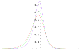
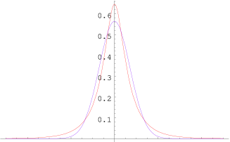
Figure 18.11. Densities of hyperbolic (red), NIG (blue) and hyperboloid distributions (left). Comparison of the GH (red) and Normal distributions (with equal mean and variance).

A typical example of the behavior of asset returns can be seen in Figures 1.2 and 18.12. The fitted normal distribution has lower peak, fatter flanks and lighter tails than the empirical distribution; this means that, in reality, tiny and large price movements occur more frequently, and small and medium size movements occur less frequently, than predicted by the normal distribution. On the other hand, the generalized hyperbolic distribution gives a very good statistical fit of the empirical distribution; this is further verified by the corresponding Q-Q plot.

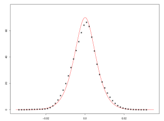
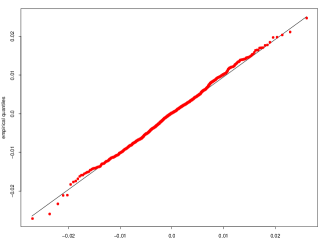
Figure 18.12. Empirical distribution and Q-Q plot of EUR/USD daily log-returns with fitted GH (red).

Under the “risk-neutral” measure, the flexibility of the generating distributions allows the implied volatility smiles produced by a Lévy model to accurately capture the shape of the implied volatility smiles observed in the market. A typical volatility surface can be seen in Figure 1.3. Figure 18.13 exhibits the volatility smile of market data (EUR/USD) and the calibrated implied volatility smile produced by the NIG distribution; clearly, the resulting smile fits the data particularly well.

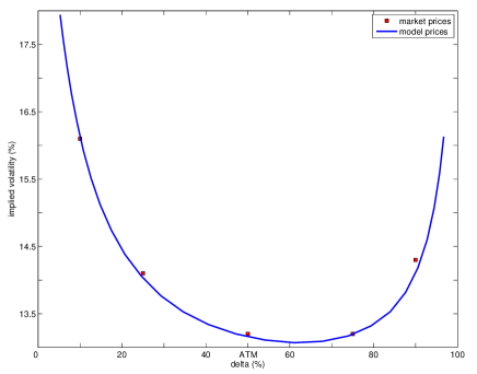
Figure 18.13. Implied volatilities of EUR/USD options and calibrated NIG smile.

Appendix A Poisson random variables and processes

Definition A.1.

Let $X$ be a Poisson distributed random variable with parameter $\lambda\in\mathbb{R}_{\geqslant 0}$. Then, for $n\in\mathbb{N}$ the probability distribution is

$$P(X=n)=\mathrm{e}^{-\lambda}\frac{\lambda^{n}}{n!}$$

and the first two centered moments are

$$\text{E}[X]=\lambda \qquad\text{and}\qquad\text{Var}[X]=\lambda.$$

Definition A.2.

A càdlàg, adapted stochastic process $N=(N_{t})_{0\leq t\leq T}$ with $N_{t}:\Omega\times\mathbb{R}_{\geqslant 0}\rightarrow\mathbb{N}\cup\{0\}$ is called a Poisson process if

1. $N_{0}=0$,

2. $N_{t}-N_{s}$ is independent of $\mathcal{F}_{s}$ for any $0\leq s<t<T$,

3. $N_{t}-N_{s}$ is Poisson distributed with parameter $\lambda(t-s)$ for any $0\leq s<t<T$.

Then, $\lambda\geq 0$ is called the intensity of the Poisson process.

Definition A.3.

Let $N$ be a Poisson process with parameter $\lambda$. We shall call the process $\overline{N}=(\overline{N}_{t})_{0\leq t\leq T}$ with $\overline{N}_{t}:\Omega\times\mathbb{R}_{\geqslant 0}\rightarrow\mathbb{R}$ where

(A.1) $$\overline{N}_{t}:=N_{t}-\lambda t$$

a compensated Poisson process.

A simulated path of a Poisson and a compensated Poisson process can be seen in Figure A.14.

Figure A.14. Plots of the Poisson (left) and compensated Poisson process.

Proposition A.4.

The compensated Poisson process defined by (A.1) is a martingale.

Proof.

We have that

1. the process $\overline{N}$ is adapted to the filtration because $N$ is adapted (by definition);

2. $\mathrm{I\kern-1.99997ptE}[|\overline{N}_{t}|]<\infty$ because $\mathrm{I\kern-1.99997ptE}[|N_{t}|]<\infty$, for all ${0\leq t\leq T}$;

3. finally, let $0\leq s<t<T$, then

   $$\mathrm{I\kern-1.99997ptE}[\overline{N}_{t}|\mathcal{F}_{s}] =\mathrm{I\kern-1.99997ptE}[N_{t}-\lambda t|\mathcal{F}_{s}]$$

   $$=\mathrm{I\kern-1.99997ptE}[N_{s}-(N_{t}-N_{s})|\mathcal{F}_{s}]-\lambda(s-(t-s))$$

   $$=N_{s}-\mathrm{I\kern-1.99997ptE}[(N_{t}-N_{s})|\mathcal{F}_{s}]-\lambda(s-(t-s))$$

   $$=N_{s}-\lambda s$$

   $$=\overline{N}_{s}.\qed$$

Remark A.5.

The characteristic functions of the Poisson and compensated Poisson random variables are respectively

$$\mathrm{I\kern-1.99997ptE}[\mathrm{e}^{iuN_{t}}]=\exp\big{[}\lambda t(\mathrm{e}^{iu}-1)\big{]}$$

and

$$\mathrm{I\kern-1.99997ptE}[\mathrm{e}^{iu\overline{N}_{t}}]=\exp\big{[}\lambda t(\mathrm{e}^{iu}-1-iu)\big{]}.$$

Appendix B Compound Poisson random variables

Let $N$ be a Poisson distributed random variable with parameter $\lambda\geq 0$ and $J=(J_{k})_{k\geq 1}$ an i.i.d. sequence of random variables with law $F$. Then, by conditioning on the number of jumps and using independence, we have that the characteristic function of a compound Poisson distributed random variable is

$$\mathrm{I\kern-1.99997ptE}\Big{[}\mathrm{e}^{iu\sum_{k=1}^{N}J_{k}}\Big{]} =\sum_{n\geq 0}\mathrm{I\kern-1.99997ptE}\Big{[}\mathrm{e}^{iu\sum_{k=1}^{N}J_{k}}\big{|}N=n\Big{]}P(N=n)$$

$$=\sum_{n\geq 0}\mathrm{I\kern-1.99997ptE}\Big{[}\mathrm{e}^{iu\sum_{k=1}^{n}J_{k}}\Big{]}\mathrm{e}^{-\lambda}\frac{\lambda^{n}}{n!}$$

$$=\sum_{n\geq 0}\left(\int_{\mathbb{R}}\mathrm{e}^{iux}F(\mathrm{d}x)\right)^{n}\mathrm{e}^{-\lambda}\frac{\lambda^{n}}{n!}$$

$$=\exp\left(\lambda\int_{\mathbb{R}}(\mathrm{e}^{iux}-1)F(\mathrm{d}x)\right).$$

Appendix C Notation

$\stackrel{{\scriptstyle\mathrm{d}}}{{=}}$ equality in law, $\mathcal{L}(X)$ law of the random variable $X$

$a\wedge b=\min\{a,b\}$, $a\vee b=\max\{a,b\}$

$\mathbb{C}\ni z=\alpha+i\beta$, with $\alpha,\beta\in\mathbb{R}$; then $\Re z=\alpha$ and $\Im z=\beta$

$1_{A}$ denotes the indicator of the generic event $A$, i.e.

$$1_{A}(x)=\left\{\begin{array}[]{ll}1,&\hbox{if $x\in A$,}\\ 0,&\hbox{if $x\notin A$.}\\ \end{array}\right.$$

Classes:

$\mathcal{M}_{\text{loc}}$ local martingales

$\mathcal{A}_{\text{loc}}$ processes of locally bounded variation

$\mathcal{V}$ processes of finite variation

$G_{\text{loc}}(\mu)$ functions integrable wrt the compensated random measure $\mu-\nu$

Appendix D Datasets

The EUR/USD implied volatility data are from 5 November 2001. The spot price was 0.93, the domestic rate (USD) 5% and the foreign rate (EUR) 4%. The data are available at

http://www.mathfinance.de/FF/sampleinputdata.txt.

The USD/JPY, EUR/USD and GBP/USD foreign exchange time series correspond to noon buying rates (dates: $22/10/1997-22/10/2004$, $4/1/99-3/3/2005$ and $1/5/2002-3/3/2005$ respectively). The data can be downloaded from

http://www.newyorkfed.org/markets/foreignex.html.

Appendix E Paul Lévy

Processes with independent and stationary increments are named Lévy processes after the French mathematician Paul Lévy (1886-1971), who made the connection with infinitely divisible laws, characterized their distributions (Lévy-Khintchine formula) and described their path structure (Lévy-Itô decomposition). Paul Lévy is one of the founding fathers of the theory of stochastic processes and made major contributions to the field of probability theory. Among others, Paul Lévy contributed to the study of Gaussian variables and processes, the law of large numbers, the central limit theorem, stable laws, infinitely divisible laws and pioneered the study of processes with independent and stationary increments.

More information about Paul Lévy and his scientific work, can be found at the websites

http://www.cmap.polytechnique.fr/ rama/levy.html

and

http://www.annales.org/archives/x/paullevy.html

(in French).

Acknowledgments

A large part of these notes was written while I was a Ph.D. student at the University of Freiburg; I am grateful to Ernst Eberlein for various interesting and illuminating discussions, and for the opportunity to present this material at several occasions. I am grateful to the various readers for their comments, corrections and suggestions. Financial support from the Deutsche Forschungsgemeinschaft (DFG, Eb 66/9-2) and the Austrian Science Fund (FWF grant Y328, START Prize) is gratefully acknowledged.

References

- [\citeauthoryearAbramowitz and StegunAbramowitz and Stegun1968] Abramowitz, M. and I. Stegun (Eds.) (1968). Handbook of Mathematical Functions (5th ed.). Dover.
- [\citeauthoryearApplebaumApplebaum2004] Applebaum, D. (2004). Lévy Processes and Stochastic Calculus. Cambridge University Press.
- [\citeauthoryearBarndorff-NielsenBarndorff-Nielsen1977] Barndorff-Nielsen, O. E. (1977). Exponentially decreasing distributions for the logarithm of particle size. Proc. R. Soc. Lond. A 353, 401–419.
- [\citeauthoryearBarndorff-NielsenBarndorff-Nielsen1997] Barndorff-Nielsen, O. E. (1997). Normal inverse Gaussian distributions and stochastic volatility modelling. Scand. J. Statist. 24, 1–13.
- [\citeauthoryearBarndorff-Nielsen, Mikosch, and ResnickBarndorff-Nielsen et al.2001] Barndorff-Nielsen, O. E., T. Mikosch, and S. Resnick (Eds.) (2001). Lévy Processes: Theory and Applications. Birkhäuser.
- [\citeauthoryearBarndorff-Nielsen and PrauseBarndorff-Nielsen and Prause2001] Barndorff-Nielsen, O. E. and K. Prause (2001). Apparent scaling. Finance Stoch. 5, 103 – 113.
- [\citeauthoryearBelomestny and ReißBelomestny and Reiß2005] Belomestny, D. and M. Reiß (2005). Optimal calibration for exponential Lévy models. WIAS Preprint No. 1017.
- [\citeauthoryearBertoinBertoin1996] Bertoin, J. (1996). Lévy processes. Cambridge University Press.
- [\citeauthoryearBlack and ScholesBlack and Scholes1973] Black, F. and M. Scholes (1973). The pricing of options and corporate liabilities. J. Polit. Econ. 81, 637–654.
- [\citeauthoryearBorovkov and NovikovBorovkov and Novikov2002] Borovkov, K. and A. Novikov (2002). On a new approach to calculating expectations for option pricing. J. Appl. Probab. 39, 889–895.
- [\citeauthoryearCarr, Geman, Madan, and YorCarr et al.2002] Carr, P., H. Geman, D. B. Madan, and M. Yor (2002). The fine structure of asset returns: an empirical investigation. J. Business 75, 305–332.
- [\citeauthoryearCarr and MadanCarr and Madan1999] Carr, P. and D. B. Madan (1999). Option valuation using the fast Fourier transform. J. Comput. Finance 2(4), 61–73.
- [\citeauthoryearContCont2001] Cont, R. (2001). Empirical properties of asset returns: stylized facts and statistical issues. Quant. Finance 1, 223–236.
- [\citeauthoryearCont and TankovCont and Tankov2003] Cont, R. and P. Tankov (2003). Financial Modelling with Jump Processes. Chapman and Hall/CRC Press.
- [\citeauthoryearCont and TankovCont and Tankov2004] Cont, R. and P. Tankov (2004). Nonparametric calibration of jump-diffusion option pricing models. J. Comput. Finance 7(3), 1–49.
- [\citeauthoryearCont and TankovCont and Tankov2006] Cont, R. and P. Tankov (2006). Retrieving Lévy processes from option prices: regularization of an ill-posed inverse problem. SIAM J. Control Optim. 45, 1–25.
- [\citeauthoryearCorcuera, Nualart, and SchoutensCorcuera et al.2005a] Corcuera, J. M., D. Nualart, and W. Schoutens (2005a). Completion of a Lévy market by power-jump assets. Finance Stoch. 9, 109–127.
- [\citeauthoryearCorcuera, Nualart, and SchoutensCorcuera et al.2005b] Corcuera, J. M., D. Nualart, and W. Schoutens (2005b). Moment derivatives and Lévy-type market completion. In A. Kyprianou, W. Schoutens, and P. Wilmott (Eds.), Exotic Option Pricing and Advanced Lévy Models, pp. 169–193. Wiley.
- [\citeauthoryearDevroyeDevroye1986] Devroye, L. (1986). Non-Uniform Random Variate Generation. Springer.
- [\citeauthoryearEberleinEberlein2001] Eberlein, E. (2001). Application of generalized hyperbolic Lévy motions to finance. In O. E. Barndorff-Nielsen, T. Mikosch, and S. I. Resnick (Eds.), Lévy Processes: Theory and Applications, pp. 319–336. Birkhäuser.
- [\citeauthoryearEberleinEberlein2007] Eberlein, E. (2007). Jump-type Lévy processes. In T. G. Andersen, R. A. Davis, J.-P. Kreiß, and T. Mikosch (Eds.), Handbook of Financial Time Series. Springer. (forthcoming).
- [\citeauthoryearEberlein, Glau, and PapapantoleonEberlein et al.2008] Eberlein, E., K. Glau, and A. Papapantoleon (2008). Analysis of valuation formulae and applications to exotic options in Lévy models. Preprint, TU Vienna (arXiv/0809.3405).
- [\citeauthoryearEberlein and JacodEberlein and Jacod1997] Eberlein, E. and J. Jacod (1997). On the range of options prices. Finance Stoch. 1, 131–140.
- [\citeauthoryearEberlein and KellerEberlein and Keller1995] Eberlein, E. and U. Keller (1995). Hyperbolic distributions in finance. Bernoulli 1, 281–299.
- [\citeauthoryearEberlein and ÖzkanEberlein and Özkan2003] Eberlein, E. and F. Özkan (2003). Time consistency of Lévy models. Quant. Finance 3, 40–50.
- [\citeauthoryearEberlein and PapapantoleonEberlein and Papapantoleon2005] Eberlein, E. and A. Papapantoleon (2005). Symmetries and pricing of exotic options in Lévy models. In A. Kyprianou, W. Schoutens, and P. Wilmott (Eds.), Exotic Option Pricing and Advanced Lévy Models, pp. 99–128. Wiley.
- [\citeauthoryearEberlein, Papapantoleon, and ShiryaevEberlein et al.2008] Eberlein, E., A. Papapantoleon, and A. N. Shiryaev (2008). On the duality principle in option pricing: semimartingale setting. Finance Stoch. 12, 265–292.
- [\citeauthoryearEberlein and PrauseEberlein and Prause2002] Eberlein, E. and K. Prause (2002). The generalized hyperbolic model: financial derivatives and risk measures. In H. Geman, D. Madan, S. Pliska, and T. Vorst (Eds.), Mathematical Finance – Bachelier Congress 2000, pp. 245–267. Springer.
- [\citeauthoryearEberlein and v. HammersteinEberlein and v. Hammerstein2004] Eberlein, E. and E. A. v. Hammerstein (2004). Generalized hyperbolic and inverse Gaussian distributions: limiting cases and approximation of processes. In R. Dalang, M. Dozzi, and F. Russo (Eds.), Seminar on Stochastic Analysis, Random Fields and Applications IV, Progress in Probability 58, pp. 221–264. Birkhäuser.
- [\citeauthoryearEsche and SchweizerEsche and Schweizer2005] Esche, F. and M. Schweizer (2005). Minimal entropy preserves the Lévy property: how and why. Stochastic Process. Appl. 115, 299–327.
- [\citeauthoryearGoll and KallsenGoll and Kallsen2000] Goll, T. and J. Kallsen (2000). Optimal portfolios for logarithmic utility. Stochastic Process. Appl. 89, 31–48.
- [\citeauthoryearGoll and RüschendorfGoll and Rüschendorf2001] Goll, T. and L. Rüschendorf (2001). Minimax and minimal distance martingale measures and their relationship to portfolio optimization. Finance Stoch. 5, 557–581.
- [\citeauthoryearHakala and WystupHakala and Wystup2002] Hakala, J. and U. Wystup (2002). Heston’s stochastic volatility model applied to foreign exchange options. In J. Hakala and U. Wystup (Eds.), Foreign Exchange Risk, pp. 267–282. Risk Publications.
- [\citeauthoryearJacod and ShiryaevJacod and Shiryaev2003] Jacod, J. and A. N. Shiryaev (2003). Limit Theorems for Stochastic Processes (2nd ed.). Springer.
- [\citeauthoryearKallsenKallsen2000] Kallsen, J. (2000). Optimal portfolios for exponential Lévy processes. Math. Meth. Oper. Res. 51, 357–374.
- [\citeauthoryearKallsen and ShiryaevKallsen and Shiryaev2002] Kallsen, J. and A. N. Shiryaev (2002). The cumulant process and Esscher’s change of measure. Finance Stoch. 6, 397–428.
- [\citeauthoryearKouKou2002] Kou, S. G. (2002). A jump diffusion model for option pricing. Manag. Sci. 48, 1086–1101.
- [\citeauthoryearKüchler and TappeKüchler and Tappe2008] Küchler, U. and S. Tappe (2008). Bilateral gamma distributions and processes in financial mathematics. Stochastic Process. Appl. 118, 261–283.
- [\citeauthoryearKyprianouKyprianou2006] Kyprianou, A. E. (2006). Introductory Lectures on Fluctuations of Lévy Processes with Applications. Springer.
- [\citeauthoryearKyprianou, Schoutens, and WilmottKyprianou et al.2005] Kyprianou, A. E., W. Schoutens, and P. Wilmott (Eds.) (2005). Exotic Option Pricing and Advanced Lévy Models. Wiley.
- [\citeauthoryearMadan and SenetaMadan and Seneta1990] Madan, D. B. and E. Seneta (1990). The variance gamma (VG) model for share market returns. J. Business 63, 511–524.
- [\citeauthoryearMatache, Schwab, and WihlerMatache et al.2005] Matache, A.-M., C. Schwab, and T. P. Wihler (2005). Fast numerical solution of parabolic integro-differential equations with applications in finance. SIAM J. Sci. Comput. 27, 369–393.
- [\citeauthoryearMatache, v. Petersdorff, and SchwabMatache et al.2004] Matache, A.-M., T. v. Petersdorff, and C. Schwab (2004). Fast deterministic pricing of options on Lévy driven assets. M2AN Math. Model. Numer. Anal. 38, 37–72.
- [\citeauthoryearMertonMerton1973] Merton, R. C. (1973). Theory of rational option pricing. Bell J. Econ. Manag. Sci. 4, 141–183.
- [\citeauthoryearMertonMerton1976] Merton, R. C. (1976). Option pricing with discontinuous returns. Bell J. Financ. Econ. 3, 145–166.
- [\citeauthoryearPapapantoleonPapapantoleon2007] Papapantoleon, A. (2007). Applications of semimartingales and Lévy processes in finance: duality and valuation. Ph. D. thesis, University of Freiburg.
- [\citeauthoryearPrabhuPrabhu1998] Prabhu, N. U. (1998). Stochastic Storage Processes (2nd ed.). Springer.
- [\citeauthoryearProtterProtter2004] Protter, P. (2004). Stochastic Integration and Differential Equations (3rd ed.). Springer.
- [\citeauthoryearRaibleRaible2000] Raible, S. (2000). Lévy processes in finance: theory, numerics, and empirical facts. Ph. D. thesis, University of Freiburg.
- [\citeauthoryearSamorodnitsky and TaqquSamorodnitsky and Taqqu1994] Samorodnitsky, G. and M. Taqqu (1994). Stable non-Gaussian Random Processes. Chapman and Hall.
- [\citeauthoryearSamuelsonSamuelson1965] Samuelson, P. A. (1965). Rational theory of warrant pricing. Indust. Manag. Rev. 6, 13–31.
- [\citeauthoryearSatoSato1999] Sato, K. (1999). Lévy Processes and Infinitely Divisible Distributions. Cambridge University Press.
- [\citeauthoryearSchoutensSchoutens2002] Schoutens, W. (2002). The Meixner process: theory and applications in finance. In O. E. Barndorff-Nielsen (Ed.), Mini-proceedings of the 2nd MaPhySto Conference on Lévy Processes, pp. 237–241.
- [\citeauthoryearSchoutensSchoutens2003] Schoutens, W. (2003). Lévy Processes in Finance: Pricing Financial Derivatives. Wiley.
- [\citeauthoryearSchoutens and TeugelsSchoutens and Teugels1998] Schoutens, W. and J. L. Teugels (1998). Lévy processes, polynomials and martingales. Comm. Statist. Stochastic Models 14, 335–349.
- [\citeauthoryearSelivanovSelivanov2005] Selivanov, A. V. (2005). On the martingale measures in exponential Lévy models. Theory Probab. Appl. 49, 261–274.
- [\citeauthoryearShiryaevShiryaev1999] Shiryaev, A. N. (1999). Essentials of Stochastic Finance: Facts, Models, Theory. World Scientific.
- [\citeauthoryearWebberWebber2005] Webber, N. (2005). Simulation methods with Lévy processes. In A. Kyprianou, W. Schoutens, and P. Wilmott (Eds.), Exotic Option Pricing and Advanced Lévy Models, pp. 29–49. Wiley.