[Ne II] Observations of Gas Motions in Compact and Ultracompact H II Regions

Abstract

We present high spatial and spectral resolution observations of sixteen Galactic compact and ultracompact H II regions in the [Ne II] 12.8 $\mu$m fine structure line. The small thermal width of the neon line and the high dynamic range of the maps provide an unprecedented view of the kinematics of compact and ultracompact H II regions. These observations solidify an emerging picture of the structure of ultracompact H II regions suggested in our earlier studies of G29.96 and Mon R2; systematic surface flows, rather than turbulence or bulk expansion, dominate the gas motions in the H II regions. The observations show that almost all of the sources have significant (5-20 km s^-1) velocity gradients and that most of the sources are limb-brightened. In many cases, the velocity pattern implies tangential flow along a dense shell of ionized gas. None of the observed sources clearly fits into the categories of filled expanding spheres, expanding shells, filled blister flows, or cometary H II regions formed by rapidly moving stars. Instead, the kinematics and morphologies of most of the sources lead to a picture of H II regions confined to the edges of cavities created by stellar wind ram pressure and flowing along the cavity surfaces. In sources where the radio continuum and [Ne II] morphologies agree, the majority of the ionic emission is blue-shifted relative to nearby molecular gas. This is consistent with sources lying on the near side of their natal clouds being less affected by extinction and with gas motions being predominantly outward, as is expected for pressure-driven flows.

1 Introduction

The short Kelvin-Helmholtz timescales of massive young stellar objects (YSOs) allow these objects to begin emitting ionizing photons and to excite nearby material while still embedded in their natal clouds (Lada, 1999). One of the earliest observable manifestations of newly formed OB stars is the ultracompact HII (UCHII) region. These embedded HII regions are initially small ($D{\leq}0.1~{}pc$) and dense ($n_{e}{\sim}10^{4}~{}cm^{-3}$) and have a typical emission measure (EM) $\sim$ 10⁷ pc cm^-6 (Churchwell, 2002). As HII regions evolve their sizes increase, but they are still considered to be UCHII regions as long as their emission measures (or surface brightnesses) remain high.

Since most stars with M $\geq$ 8 M_⊙ should form UCHII regions shortly after their birth, studies of UCHII regions can help us learn about physical conditions in high-mass star forming regions and the evolution of the physical conditions as the massive stars turn on. A large percentage, $\geq$ 50$\%$, of UCHII regions have cometary, core-halo or irregular morphologies (Wood & Churchwell, 1989b; Kurtz et al., 1994; Walsh et al., 1998; de Pree et al., 2005), arguing against the classical expanding sphere model of HII regions (Savedoff & Greene, 1955). In addition, statistical arguments based on the Galactic population of UCHII regions lead to estimates of the lifetime of these regions that are much longer than expected from the expanding sphere model (Wood & Churchwell, 1989a; Hoare et al., 2007). Many models have been proposed for UCHII region formation (see the review by Churchwell, 1999, and references therein), with solving the lifetime problem a major goal. However, the age of an individual UCHII region is hard to determine through observations. A number of theoretical models have been geared toward explaining both these long apparent lifetimes and the observed morphologies of UCHII regions (Hollenbach et al., 1994; Dyson et al., 1995; Redman et al., 1996; Williams et al., 1996; Redman et al., 1998).

Observations of the morphology and gas kinematics of UCHII regions can help us to constrain models for the structure and evolution of the regions much more definitively than observations of the morphology alone. The morphological type is not a unique indicator of the UCHII region physics because many models can produce similar morphologies (Tenorio-Tagle, 1979; Yorke et al., 1983; Mac Low et al., 1991; van Buren & Mac Low, 1992; Arthur & Hoare, 2006). While it is difficult to choose between different models based on the morphologies of HII regions, their kinematic signatures are very distinct. To understand the structure and evolution of the regions around the youngest massive stars, it is therefore necessary to observe gas kinematics inside UCHII regions with the highest spectral and spatial resolution. The large extinction associated with molecular clouds around UCHII regions, however, prevents direct observation at optical wavelengths and even at near-infrared wavelengths (Dopita et al., 2006). Thus, observations at longer wavelengths become crucial to UCHII region studies.

Radio interferometric observations can provide data with high angular and spectral resolution. At high enough frequencies, where non-LTE effects become less important, hydrogen radio recombination line (RRL) emission has the same dependence on the electron density as thermal free-free radio continuum emission, and the emissivities of these lines are well known. RRL observations can provide information on gas density and kinematics, and, to a limited degree, on gas temperature. However, thermal broadening of hydrogen RRLs due to the low mass of hydrogen atoms degrades the spectral resolution of radio spectroscopy. The thermal line width of the RRLs (or any hydrogen recombination lines like Br$\alpha$ and Br$\gamma$, for that matter) in an ionized region (T${}_{e}{\simeq}$10⁴ K) is $\simeq$ 20 km s^-1, comparable to the velocities of bulk flows in many sources. Furthermore, the incomplete uv sampling of radio interferometric survey can both overemphasize compact structures and, more generally limit the spatial dynamic range of the observations.

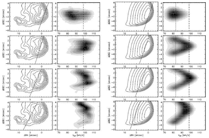
Figure 3: Position-Velocity (P-V) diagrams of G29.96 -0.02 [Ne II] observations (column 2) and a bow shock model (Zhu et al., 2005, column 4). The straight lines through the observed (column 1) and model (column 3) integrated line flux maps show the position of each cut. Dashed lines in p-v diagrams show the observed ambient molecular material velocity. Dotted lines in the model p-v diagrams show the ambient material velocity in the model. The contour maps are drawn as in Fig.1 with the peak value $\sim$1.0 ergs cm^-2 s^-1 sr^-1 for the line maps of observations.

Mid-IR fine structure line observations offer an alternative to radio and IR recombination line observations. Fine structure lines have small thermal line widths because they are emitted by heavy elements. The importance of this feature of the fine structure lines has been illustrated previously by high spectral resolution maps of [Ne II] emission in Mon R2 and G29.96-0.02 which show single lines or multiple components of lines with widths significantly smaller than the thermal widths of the hydrogen recombination lines (Jaffe et al., 2003; Zhu et al., 2005). In some cases, the broad, largely Gaussian hydrogen recombination lines are, in fact, superpositions of several much narrower kinematic components (see especially Fig. 3 of Jaffe et al. (2003)). In addition, although the emitting species are several orders of magnitude less abundant than hydrogen, the fine structure lines are brighter than recombination lines because collisional excitation cross-sections are much larger than the relevant recombination cross-sections. Typical electron densities over all compact and most ultracompact H II regions are lower than the critical density of the [Ne II] 12.8 $\mu$m transition (${\sim}5\times 10^{5}~{}cm^{-3}$), so this line shares the property of the recombination lines of having a line strength proportional to emission measure. We should mention that turbulence can also have significant effects on line widths. Moreover, turbulence affects both RRL and fine structure line observations and prevents detections of velocity variations (due to gas bulk motions) with scales smaller than the intrinsic line width combining thermal and turbulent effects along any line of sight direction.

Our previous [Ne II] line observations of a few UCHII regions have demonstrated the effectiveness of using high spectral and spatial resolution maps of fine structure lines to study such regions (Jaffe et al., 2003; Zhu et al., 2005). In these studies, we demonstrated that the kinematic patterns in the ionized gas in Mon R2 and G29.96-0.02 are consistent with tangential flows along the surfaces of thin, more-or-less parabolic shells. The goal of the current paper is to use [Ne II] mapping as a tool to examine a larger sample of compact and ultracompact HII regions with a range of shapes and sizes in order to look for a common thread in the kinematics that might lead to a better understanding of the physics and evolution of these sources. We present scan-mapped spectroscopic observations of fifteen Galactic compact and ultracompact HII regions. This survey is the first mid-infrared high-spectral resolution study of gas kinematics in a large sample of UCHII regions.

In § 2, we describe our observational method. We introduce our data reduction procedure in § 3. In § 4, we investigate the morphology and kinematics of individual objects. Finally, the conclusions drawn from our observations are presented in § 5.

2 Observations

Candidates in our survey were selected based on their radio continuum flux density levels (Wood & Churchwell, 1989b), biasing our list toward radio-bright compact and ultracompact HII regions. Observations were performed with the high spectral resolution, mid-IR (5-25 $\mu$m) cross dispersed spectrograph TEXES (Texas Echelon Cross Echelle Spectrograph, Lacy et al., 2002) on the 3.0 meter NASA IRTF on Mauna Kea in Hawaii.

We list our observational parameters in Table 1. Our spatial and spectral resolution were approximately 1.8^′′ and 4 km s^-1. For each object, a north-south oriented slit was used to scan the object from west to east. We chose the step size along the scans so that there were at least two steps per slit width and chose the scan lengths to cover the emission seen in radio continuum maps available in the literature. Before each scan, we offset the telescope to the west several arcseconds beyond the edge of the maps shown in the figures. Several extra steps were taken at the beginning and the end of each scan in order to measure the sky background. The lengths of the scans and the initial offsets were adjusted after examining a preliminary scan with our quick-look program (Lacy et al., 2002). We made multiple overlapping scans, offset north-south, to cover the sources. TEXES takes ambient temperature blackbody and sky flats at the beginning of each scan for flux calibration.

3 Data Reduction

We use a custom Fortran reduction program (Lacy et al., 2002) to correct optical distortions, flat field, remove cosmic ray spikes, and fix bad pixels. The same program also does wavelength and flux calibrations. We use atmospheric lines for wavelength calibration, with wavelengths obtained from HITRAN (Rothman et al., 1998). We use an IDL script to subtract sky background and combine multiple scans. The sky emission at each slit position is linearly interpolated from the sky frames at the beginning and the end of each scan. Sometimes, we start scans too late or end scans too early. Extended line emission is present in our sky frames and is subtracted off from other frames. This will result in an underestimate of line flux from targets. Multiple scans are cross-correlated, shifted and added to create the datacubes. Normally, no shift is needed along the spectral direction. One exception was the source W3, whose datacube was obtained by combining data from two nights and where the maps were registered using the compact continuum source IRS5 (Wynn-Williams et al., 1972). Both the Earth’s motion and the spectral settings of the instrument on two different nights affect the wavelength calibration. The continuum flux level at each pixel in the map is obtained from spectral points off the line and is subtracted from the spectra. Finally, we resample the datacubes so that each pixel has a size of $0.3^{\prime\prime}{\times}0.3^{\prime\prime}$ on the sky. The coordinates of the resulting continuum maps and [Ne II] line maps are relative to the peak positions in the integrated [Ne II] line maps. When radio continuum maps are available, they are cross-correlated with the [Ne II] maps so that both maps can be plotted on the same scale. The coordinates in Table 1 were taken from the literature and served as reference points during our line observations.

4 Results

In this section we discuss highlights of individual objects and features common to several sources. [Ne II] line emission datacubes for all objects are available online. Note: the data cubes will be available through the ApJ web site.

4.1 G29.96 -0.02

G29.96 -0.02 (G29.96 hereafter) is a cometary UCHII region at a distance of $\sim 7.4$ kpc, is $\sim$20^′′$\times$15^′′ in size, and is one of the most luminous UCHII regions in the sky at 2 cm wavelength. The ionized region is considered as an archetype of the UCHII regions caused by bow shocks (Mac Low et al., 1991), although some past observations of the gas velocities along the symmetry axis of this source argue against this interpretation, implying that the source is a blister flow (Lumsden & Hoare, 1996) or a blister flow modified by a stellar wind (Lumsden & Hoare, 1999). We presented [Ne II] line mapping observations and compared gas kinematics in the region with a bow shock model in Zhu et al. (2005). We include here a summary of the model and results for G29.96 from the earlier paper as a template for understanding the kinematics of some of the other sources in the sample. The bow shock model predicts that an approximately paraboloidal shell of swept-up material will form in front of a star moving supersonically inside a molecular cloud. The shell is supported by the ram pressure of the stellar wind and the ambient medium. Swept-up material, including ionized and neutral gas, is forced to flow along the surface of the shell. With different viewing angles for the shell, the model can reproduce many of the observed features in ionic line observations of G29.96 as well as several other UCHII regions in our sample, including morphologies and the distinctive shapes that parabolic flows have in position-velocity (p-v) diagrams.

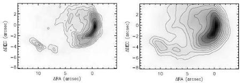
Figure 1: 2 cm continuum map (left, Fey et al., 1995, restoring beam: $0.^{\prime\prime}56\times 0.^{\prime\prime}49$) and integrated [Ne II] line map (right) of G29.96 -0.02. The (0,0) position marks the peak emission in the [Ne II] map. The line map has been cross-correlated with the continuum map and shifted to match. Contours are drawn at $70\%$, $50\%$, $35\%$, $25\%$, $17.5\%$, $12.5\%$, $9\%$ and $6\%$ of the peak value in each map. The peak [Ne II] surface brightness is 1.0 ergs cm^-2 s^-1 sr^-1. The total [Ne II] flux is 6.3$\times$10^-10 ergs cm^-2 s^-1.

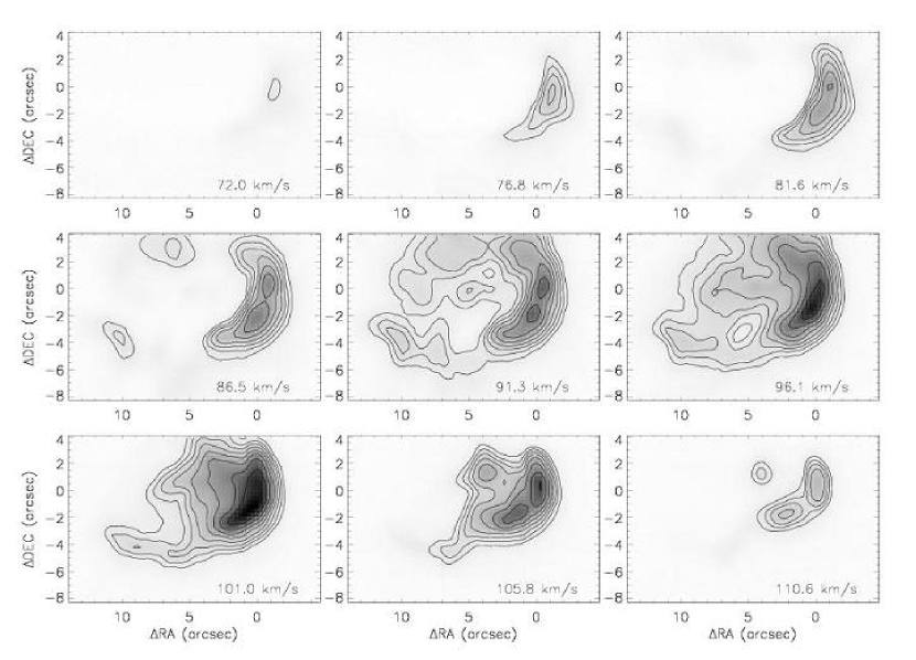
Figure 2: Channel maps of [Ne II] line observations for G29.96 -0.02. The individual maps sample a single velocity slice in the data cube and therefore represent a width equal to the spectral resolution, or about 4 km s^-1. Contours are drawn at $70\%$, $50\%$, $35\%$, $25\%$, $17.5\%$, $12.5\%$, $9\%$ and $6\%$ of the peak value of all channels. The peak value is 50.0 ergs cm^-2 s^-1 sr^-1 (cm^-1)^-1. The molecular cloud velocity is V_LSR = 98 km s^-1.

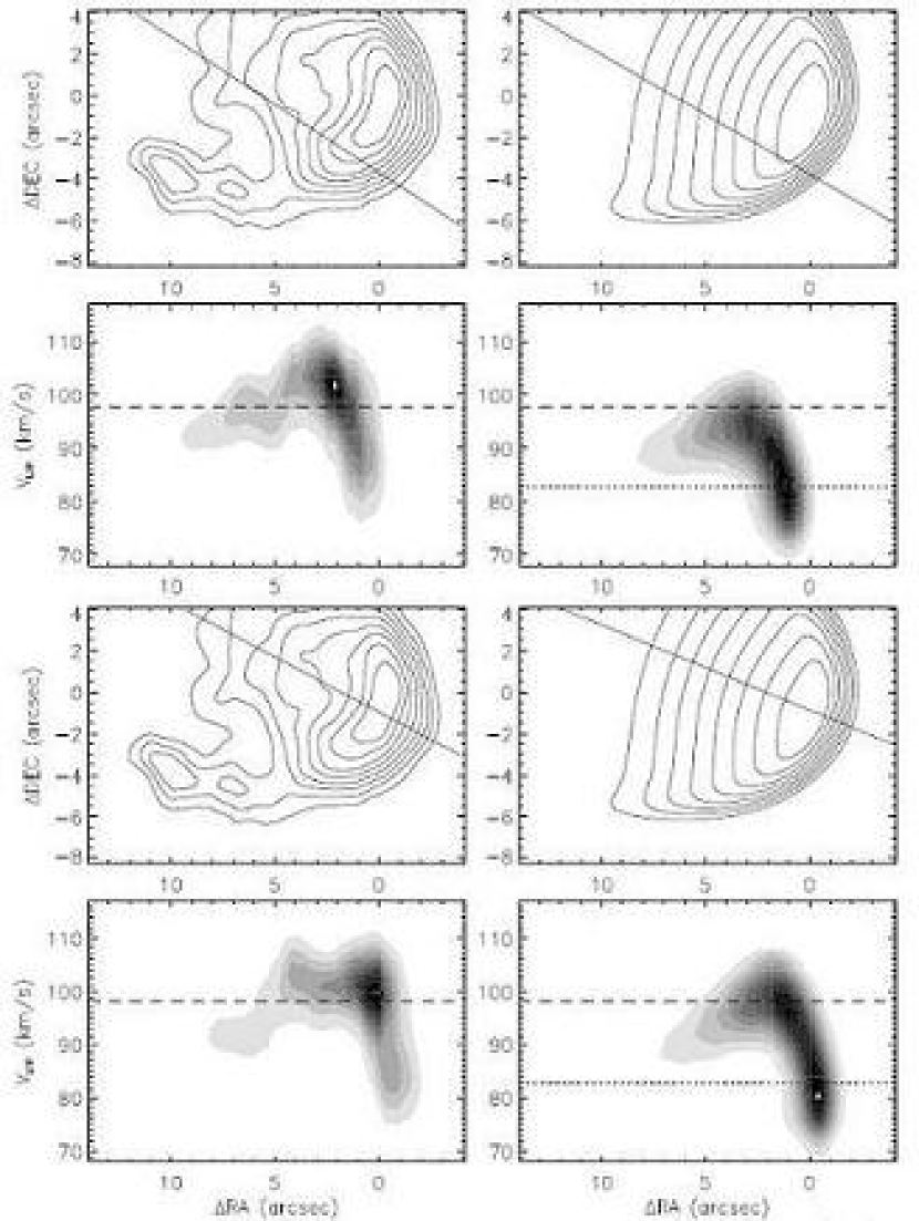
Figure 4: Position-velocity diagrams of G29.96 -0.02 [Ne II] observations (left) and the Zhu et al. (2005) bow shock model (right). The straight line in the integrated line map above each position-velocity diagram shows the location of the cut. The dashed lines in the p-v diagrams show the ambient molecular material velocity. Dotted lines in the model p-v diagrams show the ambient material velocity in the model. The contours are drawn as in Fig.1 with the peak value $\sim$1.0 ergs cm^-2 s^-1 sr^-1 for the line maps of observations.

Figure 1 shows a 2 cm radio continuum map from Fey et al. (1995) and our spectrally integrated [Ne II] line map of G29.96. The two maps closely resemble each other, indicating that most of the [Ne II] emission arises from gas with n$<$n_crit and that the extinction to the gas is either rather uniform or small at 12.8 $\mu$m. In fact, Morisset et al. (2002) observed that the electron density in the region is sub-critical (N_e$\sim$680 cm^-3 - 5.7$\times$10⁴ cm^-3) and Martín-Hernández et al. (2002) reported low infrared extinction (A_K$\simeq$1.6) toward the region. Our findings are consistent with these observations. Both maps show an emission arc open to the east with extended emission in the eastern part of the region. A filament extends from the southern edge of the nebula to the east, forming a “tail” of the cometary HII region. Channel maps at nine equally spaced velocities are shown in Figure 2. These channel maps show a morphology change from a thin crescent in the most blue-shifted channels to a fan-like region in red-shifted channels. Figures 3 and 4 show position-velocity (p-v) diagrams of several representative cross cuts made through the observed and model data cubes. The observations and the model display similar p-v structures (as shown in our previous paper, a characteristic “$\Lambda$” shape for cuts perpendicular to the nebular symmetry axis and a “7” shape for cuts parallel to the axis). Similar changes in structure from cut to cut can also be seen. The similarities in line emission morphology and gas kinematics between the observations and the model indicate that the ionized gas in G29.96 flows along a thin shell at $\sim 20$ km s^-1, as it would if it were produced by a bow shock. We use these distinctive patterns in the p-v diagrams as indicators of the presence of surface flows in other sources where we have not carried out detailed model fits. However, one clear discrepancy between the bow shock model that gives the correct shape to the contours in the model p-v diagrams in Figures 3 and 4 and the observed sources is the $\sim$15 km s^-1 difference between the observed and modeled velocity of the ambient neutral material. We discuss in § 5 modifications of the bow-shock model to explain this discrepancy.

4.2 G5.89 -0.39

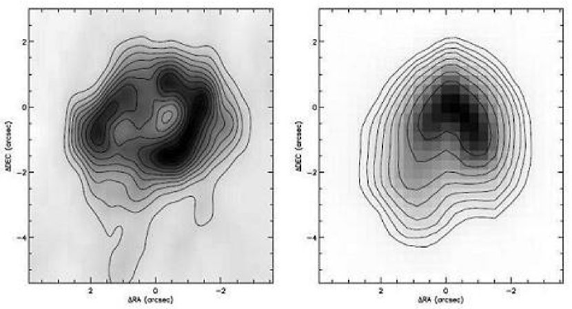
Figure 5: 6 cm continuum map (left, Wood & Churchwell, 1989b, restoring beam: $0.^{\prime\prime}38\times 0.^{\prime\prime}38$) and integrated [Ne II] line map (right) of G5.89 -0.39. The [Ne II] line map has been cross-correlated with the radio map and the (0,0) position has been shifted to the best match. The (0,0) position is the location of the emission peak in the line map. Contours are drawn at $95\%$, $90\%$, $80\%$, $70\%$, $60\%$, $50\%$, $40\%$ ,$30\%$, $20\%$ and $10\%$ of peak value for the continuum map and at $70\%$, $50\%$, $35\%$, $25\%$, $17.5\%$, $12.5\%$, $9\%$ and $6\%$ of the peak value for the line map. The peak [Ne II] surface brightness is 1.08 ergs cm^-2 s^-1 sr^-1. The total [Ne II] flux is 2.26$\times$10^-10 ergs cm^-2 s^-1.

G5.89 -0.39, also called W28 A2(1), is 2.6 kpc from the Sun (Downes et al., 1980; Kim & Koo, 2003). Wood & Churchwell (1989b) measured continuum images of the source at both 2 cm (Figure 5, left) and 6 cm. A shell-like morphology with significantly limb-brightened walls surrounding the slightly elongated central cavity can be recognized. The G5.89 region also hosts a source of extremely broad (FWHM $\sim$140 km s^-1) CO J=1-0 emission (Shepherd & Churchwell, 1996; Harvey & Forveille, 1988). Acord et al. (1998) have used multi-epoch radio continuum observations to argue that the ionized shell is expanding at $\sim$35 km s^-1. Radio recombination line observations of Rodríguez-Rico et al. (2002) show a complex velocity structure across the region, which cannot be explained with a consistent dynamical model. Mid-IR dust continuum observations show that G5.89 deviates from spherical symmetry and resembles a shell partially open to the south, with significant SW and SE protrusions from the geometric center, implying an anisotropic expansion of the ionization front due to density variations in the surrounding molecular medium (Ball et al., 1992).

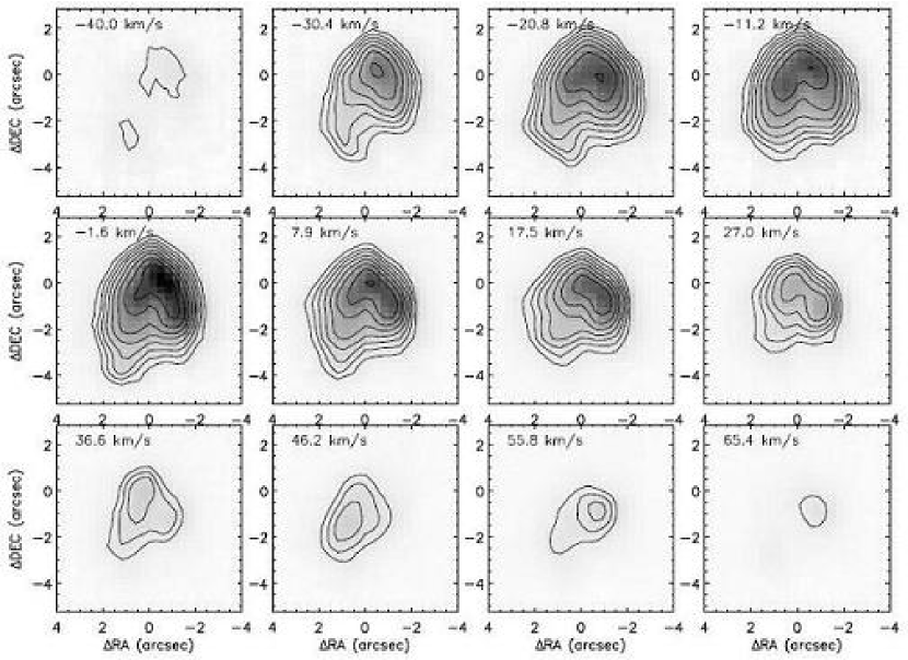
Figure 6: Channel maps of G5.89 -0.39 [Ne II] line observations. Contours are drawn at $70\%$, $50\%$, $35\%$, $25\%$, $17.5\%$, $12.5\%$, $9\%$ and $6\%$ of the peak value of all channels. The peak value is 9.15 ergs cm^-2 s^-1 sr^-1 (cm^-1)^-1. The molecular cloud velocity is V_LSR = 9 km s^-1.

Our [Ne II] 12.8 $\mu$m line map (Figure 5, right) shows a morphology similar to that of the mid-infrared continuum, with a bright arc along the north side of the source. With our $\sim 1.5^{\prime\prime}$ resolution, the kinematic signature of an expanding shell is not apparent, although there is some evidence that the line is broadest toward the center of the source (Figure 6). The majority of the emission is blue-shifted by $\sim$9 km s^-1 with respect to the molecular cloud (Hatchell et al., 1998), and the extent of the region becomes relatively smaller toward the red end of the spectrum.

4.3 G11.94 -0.62

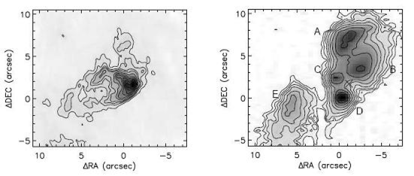
Figure 7: 2 cm continuum map (left, Wood & Churchwell, 1989b, restoring beam: $0.^{\prime\prime}41\times 0.^{\prime\prime}41$) and integrated [Ne II] line flux map (right) of G11.94 -0.62. The (0,0) is the location of the peak [Ne II] line emission. The radio continuum peak, marked with an “X”, is offset 1.17^′′ west and 1.67^′′ north from the line emission peak according to De Buizer et al. (2003). Contours are drawn at $95\%$, $90\%$, $80\%$, $70\%$, $60\%$, $50\%$, $40\%$ ,$30\%$, $20\%$,$15\%$, $10\%$ and $5\%$ of the peak flux density for the continuum map and at $70\%$, $50\%$, $35\%$, $25\%$, $17.5\%$, $12.5\%$, $9\%$ and $6\%$ of the peak value for the line map. Five separate components (A, B, C, D and E) are indicated in the line map. The peak [Ne II] surface brightness is 0.073 ergs cm^-2 s^-1 sr^-1. The total [Ne II] flux is 6.3$\times$10^-11 ergs cm^-2 s^-1.

Located at a distance of 4.2 kpc (Churchwell et al., 1990), G11.94 -0.62 was categorized by Wood & Churchwell (1989b) as a cometary UCHII region. In their radio continuum map (Figure 7, left), the region shows an emission arc with its apex pointing to the west and diffuse emission extending to the east and north. A broad ¹²CO(J=1-0) line was observed toward the object (Shepherd & Churchwell, 1996). The CO line width (full width at zero intensity) of over 28 km s^-1 suggests the presence of high velocity outflows. De Buizer et al. (2003) imaged the region at 11.7 $\mu$m and 20.8 $\mu$m. The region does not show a cometary shape in their mid-IR images and, although their pointing has an astrometric accuracy about 1^′′, the radio peak does not match any structure in the mid-IR images. The overall appearance of the region at mid-IR and radio continuum wavelengths does not match well.

Our [Ne II] 12.8 $\mu$m line map (Figure 7, right) matches the mid-IR continuum observations (De Buizer et al., 2003) very well. By registering our map with the continuum map in De Buizer et al. (2003), we determine the position of the radio continuum peak in our map, marked with an ‘X’ at (-1.17^′′, 1.67^′′). Five separate emission peaks (designated as A-E) can be seen in our integrated [Ne II] map. They all have corresponding 11.7$\mu$m and 20.8$\mu$m emission peaks in De Buizer et al. (2003). Linear sizes of these clumps range from $\sim$2^′′ in C to over 7^′′ in A and E. Like the mid-IR continuum, the [Ne II] morphology is a poor match to that of the radio continuum.

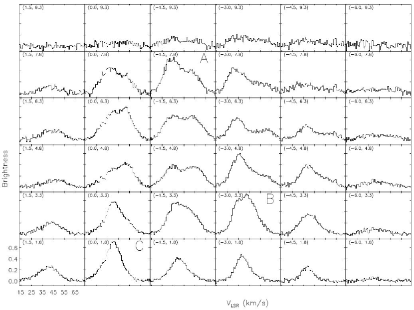
Figure 8: [Ne II] line profiles across G11.94 -0.62 (A, B and C). Spectra are averages over 1.5^′′ $\times 1.5^{\prime\prime}$. Central coordinates of the averaging areas are shown in parentheses. The brightness has units of erg cm^-2 s^-1 sr^-1 (cm^-1)^-1. The pixel size along the spectral direction is 0.0025 cm^-1 ($\sim$0.95 km s^-1). The molecular cloud velocity is V_LSR = 39 km s^-1.

The spectra of the clumps C, D and E each can be fit with a single Gaussian profile with a center velocity very close to the molecular cloud velocity (V${}_{LSR}\simeq$39 km s^-1, Churchwell et al., 1990). Figure 8 shows line profiles in the region of A, B and C. Over this part of the source, the lines are broad, with most of the additional emission to the red of the cloud velocity. The profiles in Figure 8 show that most of the [Ne II] emission occurs over the range V_LSR = 30-60 km s^-1. Complex morphology, probably induced by dust extinction, prevents a detailed analysis of the kinematics in the region.

4.4 G30.54 +0.02

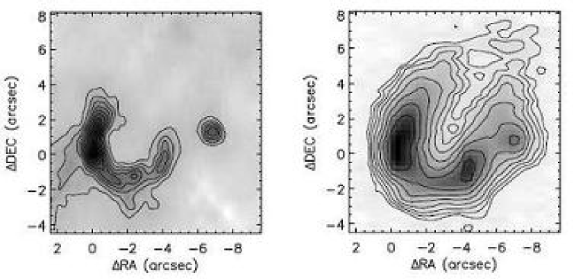
Figure 9: 2 cm continuum map (left, Wood & Churchwell, 1989b, restoring beam: $0.^{\prime\prime}41\times 0.^{\prime\prime}41$) and integrated [Ne II] line map (right) of G30.54 +0.02. The [Ne II] line map is cross-correlated with the continuum map and shifted to the best match. The (0,0) position marks the peak emission in the line map. Contours are drawn at $95\%$, $90\%$, $80\%$, $70\%$, $60\%$, $50\%$, $40\%$ ,$30\%$, $20\%$ and $10\%$ of the peak value for the continuum map and at $70\%$, $50\%$, $35\%$, $25\%$, $17.5\%$, $12.5\%$, $9\%$ and $6\%$ of the peak value for the line map The peak [Ne II] surface brightness is 0.086 ergs cm^-2 s^-1 sr^-1. The total [Ne II] flux is 4.8$\times$10^-11 ergs cm^-2 s^-1.

G30.54 +0.02 has a limb-brightened, or ”horseshoe” shape in both the radio continuum map (Wood & Churchwell, 1989b) and our [Ne II] line map (Figure 9). The more concentrated emission with a bigger opening in the radio continuum map probably is the result of the higher resolution of the interferometer observations and of the uneven sensitivity of the snapshot mode aperture synthesis to compact and extended emission. Both radio and [Ne II] line observations show that the emission arc breaks into at least three components.

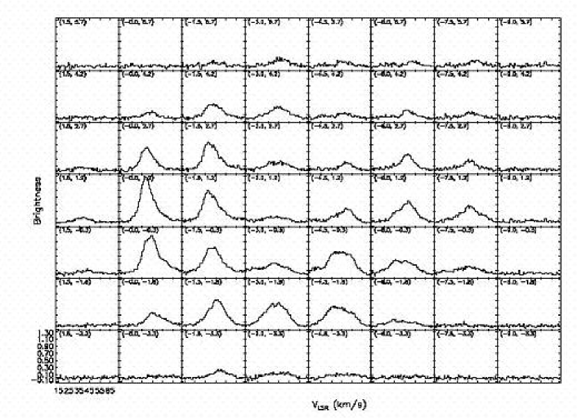
Figure 10: [Ne II] line profiles for G30.54 +0.02. Spectra are averages over $1.5^{\prime\prime}\times 1.5^{\prime\prime}$. Central coordinates of the averaging areas are shown in parentheses. The brightness has units of erg cm^-2 s^-1 sr^-1 (cm^-1)^-1. The pixel size along the spectral direction is 0.0025 cm^-1. The molecular cloud velocity is V_LSR = 48 km s^-1.

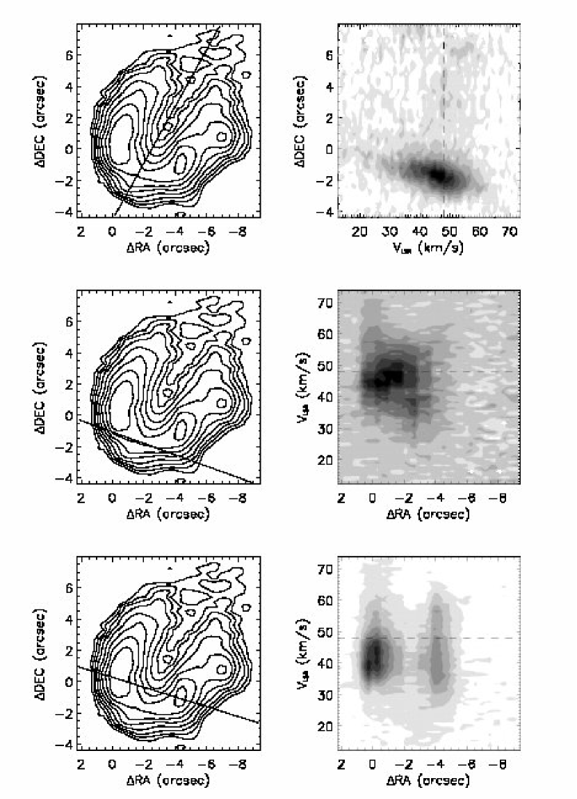
Figure 11: Position-velocity diagrams of G30.54 +0.02. Contours in line flux maps are drawn at $70\%$, $50\%$, $35\%$, $25\%$, $17.5\%$, $12.5\%$, $9\%$ and $6\%$ of the peak value (0.086 ergs cm^-2 s^-1 sr^-1). Dashed lines in p-v diagrams show the ambient molecular material velocity.

Figure 10 shows [Ne II] profiles across the region while Figure 11 displays position-velocity diagrams on selected cuts along and across the symmetry axis. Large line widths (20-30 km s^-1 FWHM), together with smooth profiles imply that turbulence or substantial small-scale motions are present and may mask the bulk motion of the gas. Nevertheless, a change of velocity pattern within the structure is still apparent.

The velocity pattern along the bright arc is consistent with significant tangential flows of the type seen in G29.96, but here mostly in the plane of the sky. At the vertex of the horseshoe, there is a single broad line with a velocity centroid close to the molecular cloud velocity (Figure 11). On the arm of the horseshoe to the east of the vertex the line peak shifts $\sim$ 7 km s^-1 to the blue of the molecular cloud velocity while on the western arm the molecular line and [Ne II] peak velocities agree. [Ne II] emission is present over at least 40-50 km s^-1 at all positions (Figures 10 and 11).

Along the symmetry axis and away from the bright arc, the match to a tangential flow is less clear. Rather than breaking up into two narrow lines, the emission on the axis and behind the vertex is at a single velocity close to that of the molecular cloud. A small velocity gradient across the apex may indicate an inclination to the plane of sky.

4.5 G33.92 +0.11

G33.92 +0.11 is particularly remarkable because of the apparent disconnect between its nondescript morphology and its distinctive position-velocity structure. It was first categorized as a core-halo UCHII region by Wood & Churchwell (1989b) and later as a shell UCHII region by Fey et al. (1992). Fey et al. (1992) showed that the 20 cm extended emission is roughly shell-like, although the cavity in their 20 cm image is offset to the southeast of the emission peak, and the rest of the region has a morphology close to a core-halo region with cometary extended emission. C¹⁸O observations showed two emission cores, and one of them is associated with the peak of the UCHII region (Watt & Mundy, 1999).

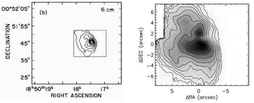
Figure 12: 6 cm continuum map (left, Fey et al., 1992, restoring beam: $1.^{\prime\prime}6\times 1.^{\prime\prime}4$, positions in B1950 coordinates) and integrated [Ne II] line flux map (right) of G33.92 +0.11. The box drawn with dashed lines in the continuum map indicates the approximate area covered by the [Ne II] line observations. The (0,0) position in the line map is the location of the peak [Ne II] line emission. Contours were drawn at $100\%$, $90\%$, $80\%$, $70\%$, $60\%$, $50\%$, $40\%$, $30\%$, $20\%$, $10\%$ and $5\%$ of the peak value for the 6 cm continuum map and at $70\%$, $50\%$, $35\%$, $25\%$, $17.5\%$, $12.5\%$, $9\%$ and $6\%$ of the peak value for the [Ne II] line map. The peak [Ne II] surface brightness is 0.24 ergs cm^-2 s^-1 sr^-1. The total [Ne II] flux is 2.7$\times$10^-10 ergs cm^-2 s^-1.

The integrated [Ne II] line map shows an irregular peak surrounded by extended emission (Figure 12). Mid-infrared continuum observations show similar structure to that seen in the [Ne II] line observations (Giveon et al., 2007). The major structure is a resolved ellipsoid oriented northeast-southwest with an additional extension to the east along the minor axis. The [Ne II] and radio continuum maps look very similar, but the central peak splits into two components in the neon line, possibly as a result of foreground extinction.

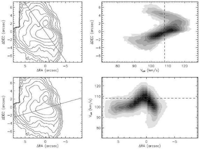
Figure 13: Position-velocity diagrams of [Ne II] observations toward G33.92 +0.11. Contours in line flux maps are drawn at $70\%$, $50\%$, $35\%$, $25\%$, $17.5\%$, $12.5\%$, $9\%$ and $6\%$ of the peak values (0.24 ergs cm^-2 s^-1 sr^-1) of the maps. Dashed lines in p-v diagrams show the ambient molecular material velocity.

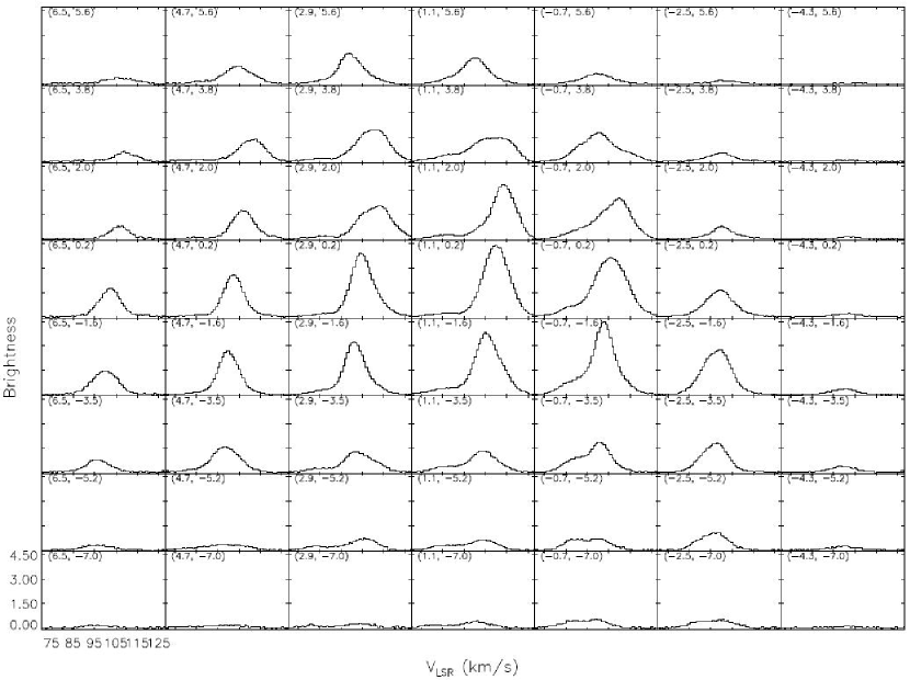
Figure 14: [Ne II] line profiles for G33.92 +0.11. Spectra are made by averaging spectra over $1.8^{\prime\prime}\times 1.8^{\prime\prime}$. Central coordinates of the averaging areas are shown in parentheses. The brightness has units of erg cm^-2 s^-1 sr^-1 (cm^-1)^-1. The pixel size along the spectral direction is 0.0025 cm^-1.

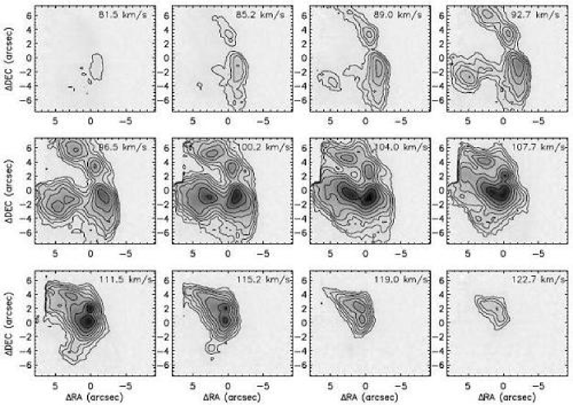
Figure 15: Channel maps of [Ne II] line observations for G33.92 +0.11. Contours are drawn at $70\%$, $50\%$, $35\%$, $25\%$, $17.5\%$, $12.5\%$, $9\%$ and $6\%$ of the peak value (5.9 ergs cm^-2 s^-1 sr^-1 (cm^-1)^-1). The molecular cloud velocity is V_LSR = 108 km s^-1.

Position-velocity diagrams along a few cross cuts through G33.92 (Figure 13) show kinematics identifiable with the kinematics typical of a flow along a surface similar to that seen in G29.96 including the characteristic “7” and “$\Lambda$” patterns, despite its more nondescript morphology. Profiles at individual positions are broad and frequently asymmetric (Figure 14). Channel maps (Figure 15) show that three prominent components form an arc at blue velocities and persist to the ambient material velocity, V${}_{LSR}\simeq$108 km s^-1. This arc has a sharp falloff to the west. A fourth emission peak and extended emission can be seen to the east of the arc. The positions of these emission peaks shift from channel to channel. This position shift is especially prominent for the peak to the east of the arc. It moves almost 5^′′ southeast from a position close to the arc in the channel at V${}_{LSR}{\simeq}$107 km s^-1 to (+6,-3) in the channel at V${}_{LSR}{\simeq}$89 km s^-1. The three components along the arc move a smaller distance to the northwest. Towards the red end of the spectrum, the emission components merge together and fade away. We note that the overall shape of the region changes from a thin crescent at blue-shifted velocities to a fan at red-shifted velocities. Bow shock models, like that for G29.96 predict a similar morphological change.

4.6 G43.89 -0.78

G43.89 -0.78 was classified as a cometary UCHII region by Wood & Churchwell (1989b). Mac Low et al. (1991) used G43.89 as one of their bow shock model tests. They concluded, based on the continuum maps that they needed a viewing angle between 45^∘ and 60^∘ from head-on in order to fit the morphology well. Shepherd & Churchwell (1996) found evidence for high-velocity molecular material in the region with a CO line width over 39 km s^-1. Low-resolution 21 $\mu$m imaging observations showed the region as a point source with extended emission to the southeast (Crowther & Conti, 2003), while the radio continuum observations showed extended emission northwest of an emission peak.

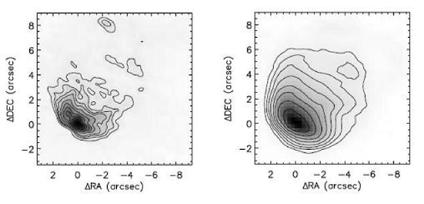
Figure 16: 2 cm continuum contour map (left, Wood & Churchwell, 1989b, restoring beam: $0.^{\prime\prime}41\times 0.^{\prime\prime}41$) and integrated [Ne II] line flux map (right) of G43.89 -0.78. The line map has been cross-correlated with the continuum map and shifted to match. The (0,0) position is the location of peak emission in the line map. Contours are drawn at $95\%$, $90\%$, $80\%$, $70\%$, $60\%$, $50\%$, $40\%$, $30\%$, $20\%$, $15\%$, $10\%$ and $5\%$ of the peak value for the radio map and at $70\%$, $50\%$, $35\%$, $25\%$, $17.5\%$, $12.5\%$, $9\%$ and $6\%$ of the peak value for the line map. The peak [Ne II] surface brightness is 0.22 ergs cm^-2 s^-1 sr^-1. The total [Ne II] flux is 7.3$\times$10^-11 ergs cm^-2 s^-1.

The cometary morphology and kinematics of the [Ne II] line emission (Figure 16-17) are consistent with flows along the surface of the region like those seen in G29.96. We fitted the p-v diagrams with a model like that used for G29.96 (Zhu et al., 2005). The best fit was with a stellar motion of 15 km s^-1 and 140^∘ away from the direction to the observer. However, as with G29.96, there is a discrepancy between the model, which predicts that the ionic emission should be redshifted relative to the molecular emission, and the observed emission, which is predominantly blueshifted.

4.7 G45.07 +0.13

G45.07 +0.13 was classified as an UCHII region with a shell morphology by Turner & Matthews (1984). At a distance of $\sim$6.0 kpc (Churchwell et al., 1990), it has a diameter $\sim$0.9^′′ at $\lambda$=2 cm (Wood & Churchwell, 1989b). The slight velocity gradient in the H76$\alpha$ line was interpreted as the result of either an expanding ring (Garay et al., 1986) or ionized bipolar outflows (Lim & White, 1999). A group of water masers lie 2^′′ to the north of the radio continuum peak (Hofner & Churchwell, 1996; De Buizer et al., 2003).

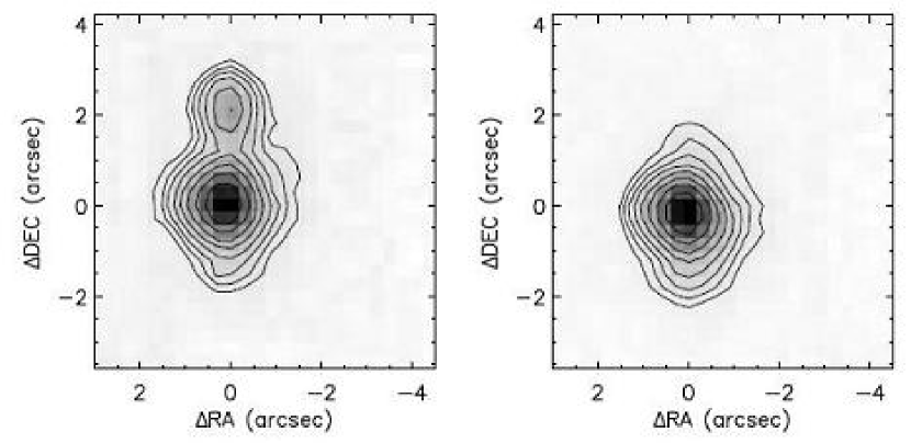
Figure 18: Dust 12.8 $\mu$m continuum map (left) and integrated [Ne II] line flux map (right) of G45.07 +0.13. The fainter northern source in the left figure is a hot molecular core candidate. The (0,0) position marks the peak [Ne II] line emission. Contours are drawn at $70\%$, $50\%$, $35\%$, $25\%$, $17.5\%$, $12.5\%$, $9\%$ and $6\%$ of peak values in both maps. The peak continuum flux density is 0.23 ergs cm^-2 s^-1 sr^-1 (cm^-1)^-1. The peak [Ne II] surface brightness is 0.14 ergs cm^-2 s^-1 sr^-1. The total [Ne II] flux is 7.8$\times$10^-12 ergs cm^-2 s^-1.

G45.07 is unresolved in our 12.8 $\mu$m [Ne II] map at 2^′′ spatial resolution (Figure 18, right). The [Ne II] line toward G45.07 is much narrower (V${}_{FWHM}\simeq$ 20 km s^-1) than is the H76$\alpha$ radio recombination line ($\sim$48 km s^-1, Garay et al., 1986). The difference in widths can arise either from pressure broadening of the H76$\alpha$ line or from the presence of high velocity material at very high density where the recombination line emissivity is proportional to n${}_{e}^{2}$ while the [Ne II] emissivity only scales with n_e. Dust continuum emission is observed at G45.07 and at a second source $\sim$2^′′ north of G45.07 (Figure 18, left). The location of the second source matches the positions of the H₂O masers. We did not detect any line emission from the second source, supporting the suggestion that this source is at an early evolutionary stage (Hofner & Churchwell, 1996; De Buizer et al., 2003).

4.8 G45.12 +0.13

G45.12 +0.13 (G45.12 hereafter) is located at a distance of 6.9 kpc (Churchwell et al., 1990). It was observed by Wood & Churchwell (1989b) with the VLA at 2 and 6 cm and revealed at least 3 peaks with a roughly arc-like overall morphology.

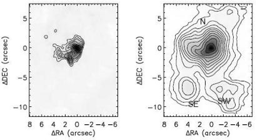
Figure 19: 2 cm continuum map (left, Wood & Churchwell, 1989b, restoring beam: $0.^{\prime\prime}41\times 0.^{\prime\prime}41$) and integrated [Ne II] line map (right) of G45.12 +0.13. The (0,0) position is the location of the [Ne II] line emission peak. The contours are drawn at $95\%$, $90\%$, $80\%$, $70\%$, $60\%$, $50\%$, $40\%$ ,$30\%$, $20\%$,$15\%$, $10\%$ and $5\%$ of peak value for the radio continuum map and at $70\%$, $50\%$, $35\%$, $25\%$, $17.5\%$, $12.5\%$, $9\%$, $6\%$, $4\%$, $2\%$ and $1\%$ of the peak value for the [Ne II] map. The peak [Ne II] surface brightness is 1.2 ergs cm^-2 s^-1 sr^-1. The total [Ne II] flux is 4.5$\times$10^-10 ergs cm^-2 s^-1.

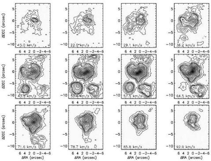
Figure 20: Channel maps for G45.12 +0.13. Contours are drawn at $70\%$, $50\%$, $35\%$, $25\%$, $17.5\%$, $12.5\%$, $9\%$, $6\%$, $4\%$, $2\%$ and $1\%$ of the peak value of all channels. The peak value is 11.1 ergs cm^-2 s^-1 sr^-1 (cm^-1)^-1. The molecular cloud velocity is V_LSR = 59 km s^-1.

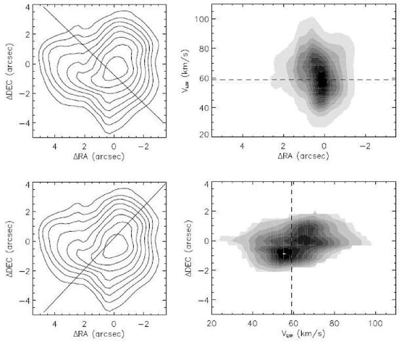
Figure 21: Position-velocity diagrams of G45.12 +0.13N. Contours in line flux maps are drawn at $70\%$, $50\%$, $35\%$, $25\%$, $17.5\%$, $12.5\%$, $9\%$ and $6\%$ of the peak values (1.23 ergs cm^-2 s^-1 sr^-1) in the maps. Dashed lines in p-v diagrams show the ambient molecular material velocity.

Our [Ne II] line observations do not completely resolve the three components along the radio emission arc, which is only $\sim$3” long (referred to as Source “N” in Figure 19). The channel maps (Figure 20) show that the “horns” of the arc-like structure are more prominent at lower redshifts while the bright spot at the middle of the arc dominates at higher velocities. The p-v diagrams of a cut parallel to the symmetry axis of the source N do show “7” patterns of cometary H II regions (Figure 21, top panels), but a cut perpendicular to the axis does not show the expected “$\Lambda$” shaped pattern (Figure 21, bottom panels). It is not clear how much the kinematics in G45.12N resembles that in a cometary HII region, because its “7” type p-v diagram is not dramatic compared to that in G29.96 (Figure 3).

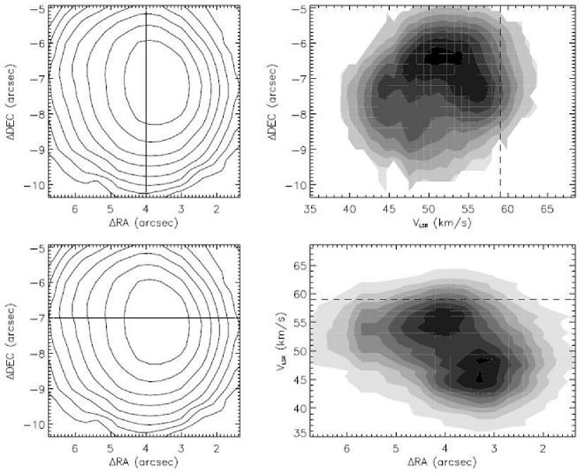
Figure 22: Position-velocity diagrams of G45.12 +0.13SE. Contours in line flux maps are drawn at $70\%$, $50\%$, $35\%$, $25\%$, $17.5\%$, $12.5\%$, $9\%$ and $6\%$ of the peak values (0.10 ergs cm^-2 s^-1 sr^-1) in the maps. Dashed lines in p-v diagrams show the ambient molecular material velocity.

We also find two fainter sources to the south of the arc which were not seen in the sparsely sampled VLA snapshot image. To show these two faint sources clearly, we extend contour levels down to 1$\%$ of the peak value in our line map. The southeastern source (SE) is extended and almost round-shaped. It is hard to determine its symmetry axes. Its p-v diagrams along RA and DEC cuts (Figure 22) show evidence of gas bulk motion and most of emission is blue-shifted relative to the ambient molecular gas. Tentative “7” shaped emission distribution can be seen in these diagrams, suggesting that surface flows may be present in the source. The southwestern source (SW) is irregular and contains multiple peaks. These emission peaks surround an emission minimum at the same location $\sim$(2.^′′7, -8^′′) in almost all channels (Figure 20). A broken shell-like morphology with an opening to the west suggests an expanding shell structure for SW, but the ring of the line emission does not collapse at the ends of the Doppler shift-range as would be expected for an expanding shell. The velocity distributions in both N and SW are more or less symmetric about the ambient material velocity, which is 59 km s^-1. Line emission from SE is relatively blue-shifted, and the width of the [Ne II] line is narrower in SE than in the other two sources.

4.9 G45.45 +0.06

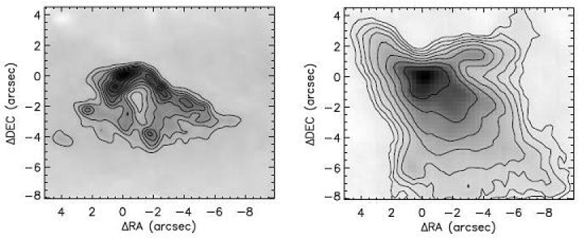
Figure 23: 6 cm continuum map (left, Wood & Churchwell, 1989b, restoring beam: $0.^{\prime\prime}38\times 0.^{\prime\prime}38$) and integrated [Ne II] line map (right) of G45.45 +0.06. The [Ne II] line map has been cross-correlated with the radio map and the (0,0) position has been shifted to the best match. The (0,0) position is the location of the emission peak in the line map. Contours are drawn at $95\%$, $90\%$, $80\%$, $70\%$, $60\%$, $50\%$, $40\%$ ,$30\%$, $20\%$ and $10\%$ of peak value for the continuum map and at $70\%$, $50\%$, $35\%$, $25\%$, $17.5\%$, $12.5\%$, $9\%$ and $6\%$ of the peak value for the line map. The peak [Ne II] surface brightness is 0.16 ergs cm^-2 s^-1 sr^-1. The total [Ne II] flux is 1.2$\times$10^-10 ergs cm^-2 s^-1.

G45.45 +0.06 was categorized by Wood & Churchwell (1989b) as a cometary UCHII region. In the 6 cm radio continuum image, the source extends $\sim 9^{\prime\prime}$ EW and $6^{\prime\prime}$ NS and has a sharp and bright ionization front to the north and extended emission to the south (Figure 23, left panel). Multiple emission peaks arranged along the ionization front form a distorted ring around a cavity. At a distance 6.6 kpc, the integrated continuum flux density implies an O7.5 main sequence star as the ionizing star (Churchwell et al., 1990). Feldt et al. (1998) acquired images at H and K^′ bands and three mid-infrared bands centered at 3.8$\mu$m, 10.5$\mu$m and 11.7$\mu$m and found that the region contained a young OB cluster.

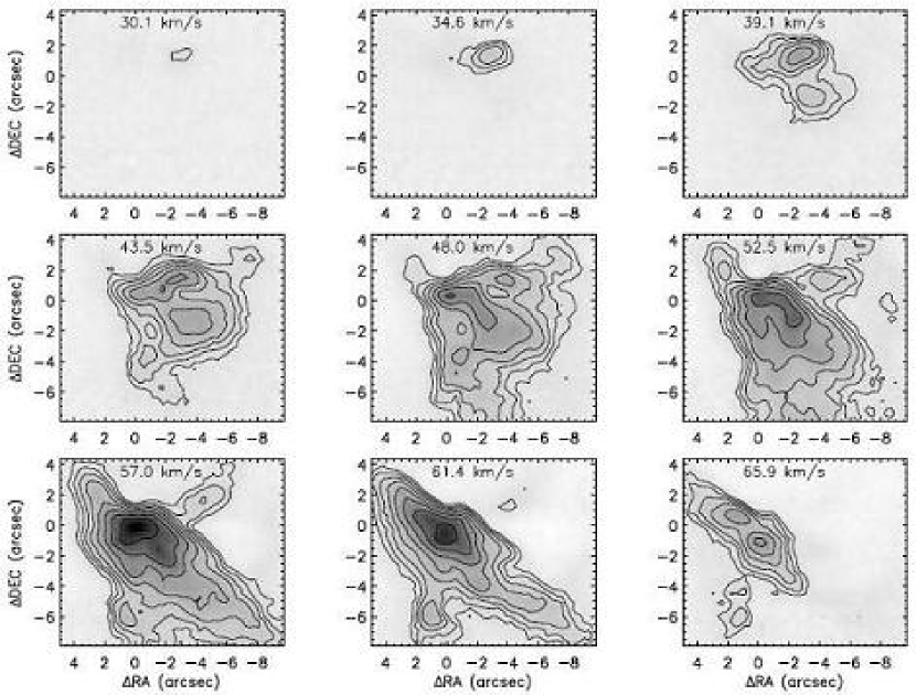
Figure 24: Channel maps for G45.45 +0.06 [Ne II] line observations. Contours are drawn at $70\%$, $50\%$, $35\%$, $25\%$, $17.5\%$, $12.5\%$, $9\%$ and $6\%$ of the peak value of all channels. The peak value is 4.2 ergs cm^-2 s^-1 sr^-1 (cm^-1)^-1. The molecular cloud velocity is V_LSR = 59 km s^-1.

The overall morphology of the [Ne II] line emission (Figure 23, right) does not look like that of the radio continuum map. Most of the line emission comes from an elongated structure aligned northeast to southwest with the extended emission to the southwest roughly matching that seen in Br$\gamma$ by Feldt et al. (1998). The intermediate velocity (43-53 km s^-1) channel maps (Figure 24) most nearly match the radio emission. The NE-SW elongated structure is primarily present in red-shifted velocity channels. Extended emission north of the radio arc and a overlying compact 11.7 $\mu$m source (Feldt et al., 1998) dominate the blue-shifted channels. The differences between the [Ne II] and radio distributions could be due to incomplete uv coverage of the snap shot radio observations or/and to greater sensitivity of [Ne II] line observations.

4.10 W51 IRS2

W51 IRS2 (W51d) is a luminous (L = 2-4 $\times$10⁶ L_⊙, Erickson & Tokunaga, 1980; Jaffe et al., 1987) ultracompact HII region/molecular cloud core within a more extensive star forming complex (Carpenter & Sanders 1998). Proper motion studies of H₂O maser features place W51 IRS2 at a distance of $\sim$ 7 kpc (Genzel et al., 1981; Schneps et al., 1981; Imai et al., 2002). Elsewhere, we have presented 0.5^′′ resolution maps of the [S IV] 10.5 $\mu$m and [Ne II] 12.8 $\mu$m lines toward this source (Lacy et al., 2007). These maps reveal a number of embedded UCHII regions, which dominate the [Ne II] emission, a more extensive surface flow, seen mostly in [S IV], and a prominent $\sim$ 100 km s^-1 jet, which we attribute to ionization of one lobe of a protostellar jet. The surface flow has a position-velocity pattern indicating that the gas is moving along a shell with its vertex pointed away from the observer. At the shell edges, the emission is blue shifted by 10-15 km s^-1 with respect to the ambient cloud. The flow is less evident in [Ne II] where several compact sources are much brighter, either because of the lower extinction at 12.8 $\mu$m or because of the lower ionization potential of neon than of S⁺⁺.

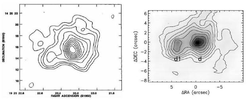
Figure 25: 2 cm continuum map (left, Gaume & Mutel, 1987, resolution: $1.^{\prime\prime}2$) and integrated [Ne II] line flux map (right) of W51 IRS2. Contours in the radio map were drawn at $90\%$, $80\%$, $70\%$, $60\%$, $50\%$, $40\%$, $30\%$ ,$20\%$, $10\%$ and $-10\%$ of the peak value. Contours in the [Ne II] map are drawn at $70\%$, $50\%$, $35\%$, $25\%$, $17.5\%$, $12.5\%$, $9\%$ and $6\%$ of peak line emission at (0,0). The peak [Ne II] surface brightness is 0.66 ergs cm^-2 s^-1 sr^-1. The total [Ne II] flux is 4.2$\times$10^-10 ergs cm^-2 s^-1.

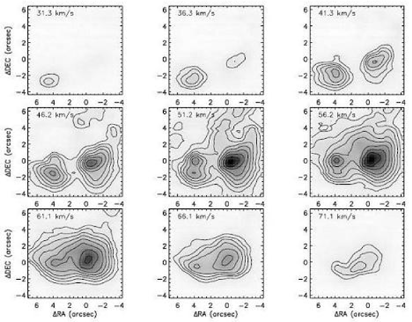
Figure 26: Channel maps of W51 IRS2 [Ne II] line observations. Contours are drawn at $70\%$, $50\%$, $35\%$, $25\%$, $17.5\%$, $12.5\%$, $9\%$ and $6\%$ of the peak value of all channels. The peak value is 13.2 ergs cm^-2 s^-1 sr^-1 (cm^-1)^-1. The molecular cloud velocity is V_LSR = 58 km s^-1.

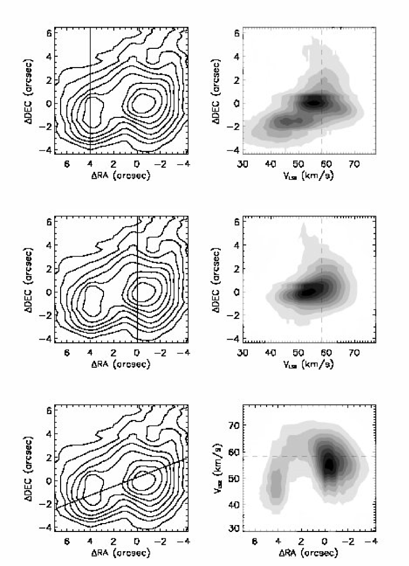
Figure 27: Position-velocity diagrams of W51 IRS2 [Ne II] line observations. Contours in line flux maps are drawn at $70\%$, $50\%$, $35\%$, $25\%$, $17.5\%$, $12.5\%$, $9\%$ and $6\%$ of peak values (0.66 ergs cm^-2 s^-1 sr^-1) of the maps. Dashed lines in p-v diagrams show the ambient molecular material velocity.

We include our somewhat more extensive 2^′′ resolution IRTF map of W51 IRS2 in the [Ne II] line here for completeness. Figure 25 compares the distribution of radio continuum and [Ne II] emission. The channel maps in Figure 26, as well as the top p-v diagram in Figure 27 show that the two components of the eastern source d1 have velocities that differ by $\sim$ 10 km s^-1, with the southern component blueshifted by $\sim$ 12 km s^-1 from the molecular cloud velocity. The molecular emission spectra of CS show a second feature close to the [Ne II] velocity in the southern component (49.5 km s^-1, Plume et al. 1997). The northern component of W51d1 and W51d have [Ne II] velocities close to the velocity of the main component of the molecular cloud. We also notice that the ionized gas toward the center of the region is somewhat redshifted with respect to ambient material, which is likely because the ionized gas is pushed into the cloud by stellar/cluster winds.

4.11 G61.48 +0.09B

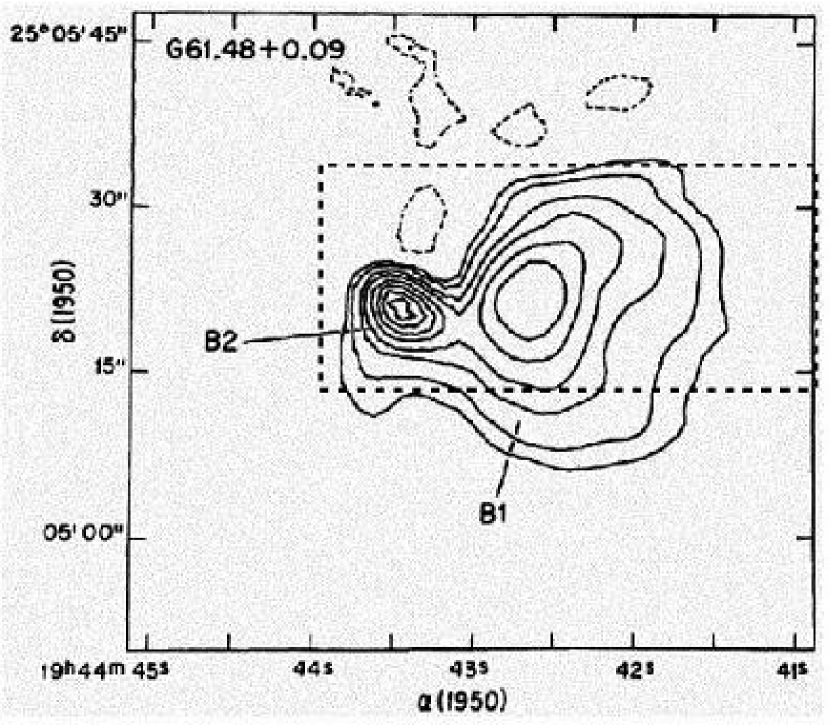
Figure 28: 1.3 cm continuum map of G61.48 +0.09 (Gomez et al., 1995, resolution $\sim 4^{\prime\prime}$). Contours were drawn at $90\%$, $75\%$, $60\%$, $45\%$, $30\%$ ,$20\%$, $10\%$, $5\%$ and $-5\%$ of the peak value. The box drawn with dashed lines indicates the approximate area covered by our [Ne II] observations.

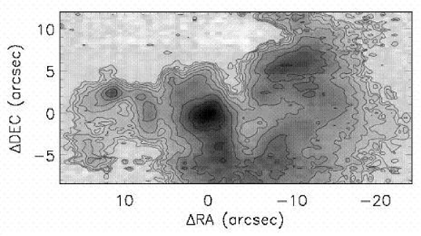
Figure 29: Integrated [Ne II] line flux map of G61.48 +0.09. The (0,0) position is the location of the [Ne II] line emission peak. Contours are drawn at $70\%$, $50\%$, $35\%$, $25\%$, $17.5\%$, $12.5\%$, $9\%$ and $6\%$ of the peak value. The peak [Ne II] surface brightness is 0.052 ergs cm^-2 s^-1 sr^-1. The total [Ne II] flux is 2.2$\times$10^-10 ergs cm^-2 s^-1.

G61.48 +0.09B belongs to the emission nebula complex Sh2-88B at a distance of 5.4 kpc (Churchwell et al., 1990). Garay et al. (1994) compared kinematics from hydrogen recombination line and molecular line observations (MacDonald et al., 1981; Churchwell et al., 1990) and concluded that the region was undergoing a blister flow to the southwest. They argued that the hydrogen recombination line kinematics and the radio continuum morphology of the region were best explained by expansion of ionized gas in a non-uniform medium. Radio continuum observations show that the region consists of two components, designated as B1 and B2 in Figure 28. The more compact and spherical B2 is located $\sim$11^′′ east of the peak of B1, which is extended and has slightly curved contours that hint toward a cometary morphology. Our [Ne II] line emission distribution (Figure 29), which is very similar to the distribution of Br$\gamma$ emission (Puga et al., 2004), shows significantly different structure than the radio continuum map. The morphological difference between the [Ne II] line emission and the radio continuum emission is likely due to dust extinction. The [Ne II] emission has complex morphology and kinematics. Multiple components are present over a 35^′′ by 20^′′ area. A bright ridge of emitting gas runs diagonally from the northeast to south central in the map. A less bright irregular structure extends to the northwest from the south.

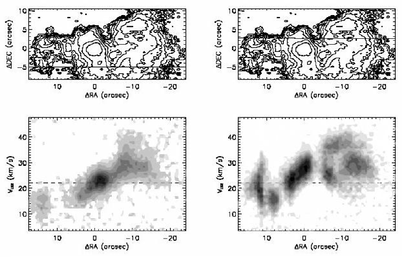
Figure 30: Position-velocity diagrams of G61.48 +0.09 [Ne II] line observations. Contours in line flux maps are drawn at $70\%$, $50\%$, $35\%$, $25\%$, $17.5\%$, $12.5\%$, $9\%$ and $6\%$ of peak values (0.052 ergs cm^-2 s^-1 sr^-1) in the maps. The spatial resolution of the map is $\sim 4^{\prime\prime}$. Dashed lines in p-v diagrams show the ambient molecular material velocity.

The p-v diagrams (Figure 30) show that the gas observable in the [Ne II] line has a steep velocity gradient. The [Ne II] emission near B2 is blueshifted by a few km s^-1 with respect to the neutral cloud velocity. Over much of B1, the bulk of the neon emission arises in redshifted material with the westernmost gas ranging from 0-20 km s^-1 to the red of the molecular line center. The morphological differences between the radio and [Ne II] maps make it difficult to associate the kinematic and morphological structures. The RRL observations of Garay et al. (1994), which are not affected by extinction, show that the bulk of the ionized material is redshifted with respect to the molecular cloud.

4.12 K3-50A (G70.3 +1.6)

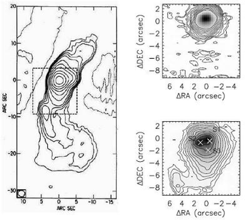
Figure 31: The 2.0 cm continuum map of K3-50A (left) (de Pree et al., 1994, resolution$\sim 1.^{\prime\prime}3$). The (0,0) position marks the peak continuum emission. First positive and negative contours were drawn at the 3$\sigma$ flux level. Other contours were drawn at 1.4, 2, 2.8, 4, 8, 16, 32, 64, 128 and 256 times the 3$\sigma$ flux level. The box drawn with dashed lines indicates the approximate area covered by our [Ne II] observations. The 12.8 $\mu$m dust continuum map (top right) and integrated [Ne II] line flux map (bottom right). For both maps, the (0,0) position is the location of the [Ne II] emission peak. Three crosses show the approximate positions of S1, S2, and S3 which are [Ne II] emission concentrations identified in the channel maps (Figure 32). Contours are drawn at $70\%$, $50\%$, $35\%$, $25\%$, $17.5\%$, $12.5\%$, $9\%$, $6\%$, $4\%$, $2\%$ and $1\%$ of the peak values in both maps. The peak dust continuum flux density is 0.82 ergs cm^-2 s^-1 sr^-1 (cm^-1)^-1. The peak [Ne II] surface brightness is 0.34 ergs cm^-2 s^-1 sr^-1. The total [Ne II] flux is 1.0$\times$10^-10 ergs cm^-2 s^-1.

K3-50 is a four-component (A-D, Wynn-Williams, 1969) HII region complex at a distance of 8.7 kpc (Harris, 1975). The kinematic distance was computed using the galactic rotational curve of Schmidt (1965) with the assumed Sun-to-GC distance of 10 kpc and a 250 km s^-1 circular velocity at the position of the Sun (Rubin & Turner, 1969; Rubin, 1965). More recent estimates of the distance to the Galactic Center ($sim$7.94 kpc) imply that this distance is too large (Eisenhauer et al., 2003). The UCHII region K3-50A appears to be the youngest and dominates the emission at infrared wavelengths. Hofmann et al. (2004) presented K^′ band bispectrum speckle interferometric data of K3-50A and their observations suggested that K3-50A is excited by a small cluster of massive to intermediate-mass stars. Radio continuum and hydrogen recombination line observations found that the ionized gas in K3-50A was undergoing a high-velocity bipolar outflow (de Pree et al., 1994). The left panel of Figure 31 shows the radio continuum image (de Pree et al., 1994). There is extended emission both north and south of the dashed box that shows the extent of the [Ne II] map.

The [Ne II] line emission in K3-50A peaks at the radio peak and has a remarkably similar distribution to that of the radio continuum within the dashed box (Figure 31). This is consistent with its relatively low extinction ($A_{K}=1.6$, Martín-Hernández et al., 2002). Most of the line emission comes from the core of the region. The integrated line map shows that the core of K3-50A consists of two sources, source 1 (S1) at the line emission peak and source 2 (S2) $\sim 1.5^{\prime\prime}$ southeast of S1. Line emission extends north and south from the central region. In the 12.8 $\mu$m continuum (Figure 31), a more compact emission peak is slightly offset ($\sim$1^′′) to the north of S1.

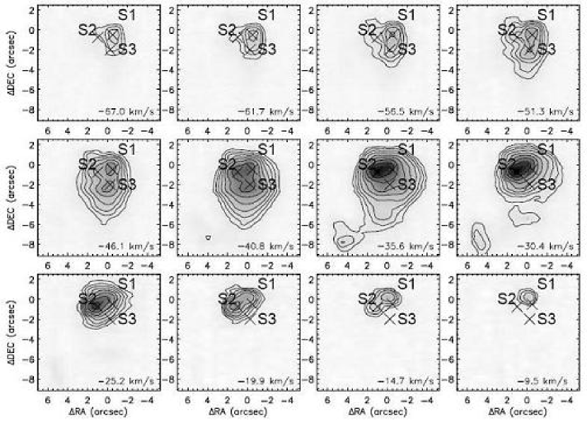
Figure 32: Channel maps of K3-50A [Ne II] line observations. Contours are drawn at $70\%$, $50\%$, $35\%$, $25\%$, $17.5\%$, $12.5\%$, $9\%$ and $6\%$ of the peak value of all channels. The peak value is 5.1 ergs cm^-2 s^-1 sr^-1 (cm^-1)^-1. The molecular cloud velocity is V_LSR = -24 km s^-1.

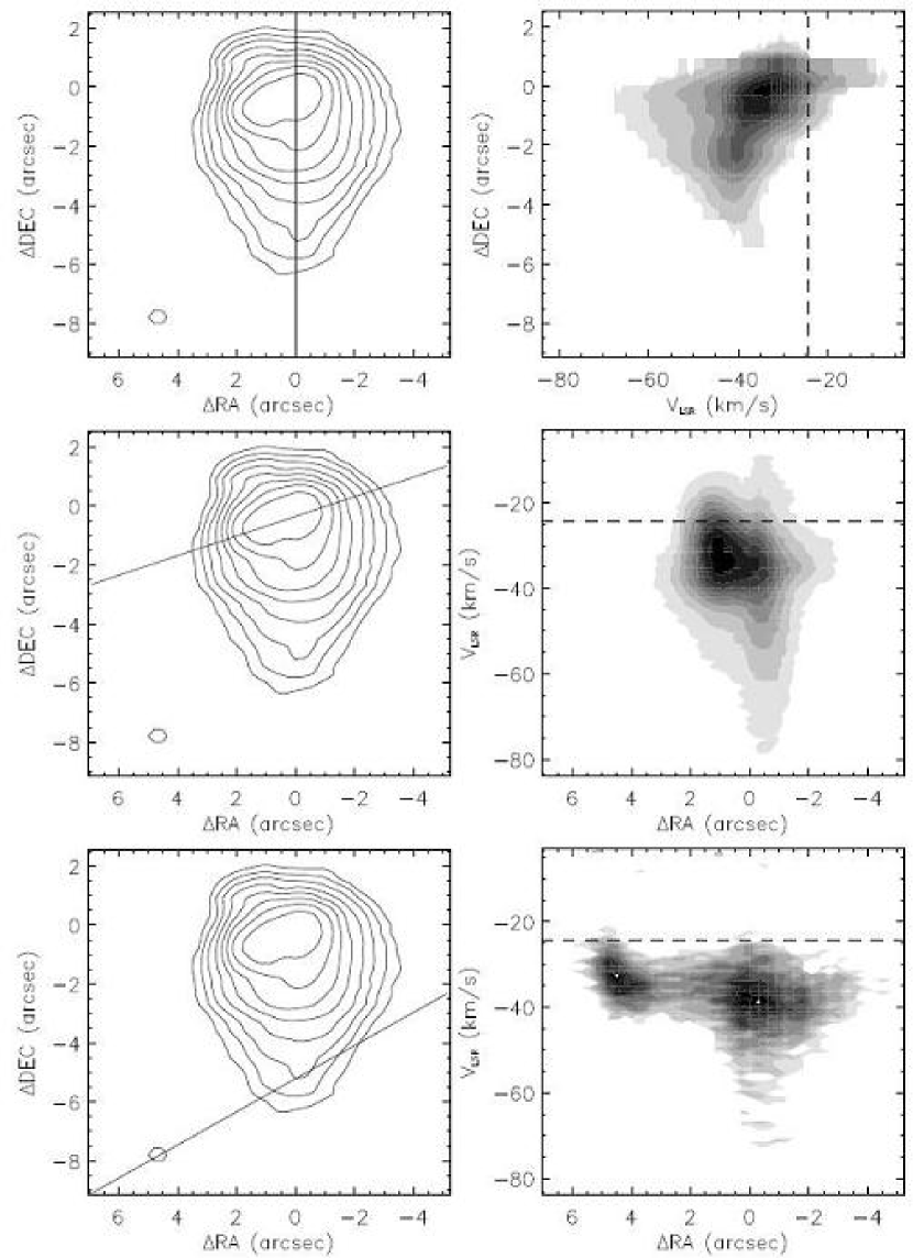
Figure 33: Position-velocity diagrams of K3-50A [Ne II] line observations. Contours in line flux maps are drawn at $70\%$, $50\%$, $35\%$, $25\%$, $17.5\%$, $12.5\%$, $9\%$ and $6\%$ of peak values (0.34 ergs cm^-2 s^-1 sr^-1) of the maps. Dashed lines in p-v diagrams show the ambient molecular material velocity.

The [Ne II] emission has a very broad velocity range, from -67 km s^-1 to -8 km s^-1 (Figure 32). S1, at (0,0), is present in all velocity channels. S2 is bright in the channels at the red end of the spectrum. A third component (S3) $\sim 2^{\prime\prime}$ to the south of S1 is present in the channels at central and blue-shifted velocities. All three components lie significantly to the blue of the molecular cloud which has V_LSR = -24 km s^-1 (Shepherd & Churchwell, 1996). S3 has the biggest velocity shift with a line center at $\sim$-39 km s^-1, with S1 and S2 at $\sim$-35 km s^-1. Position-velocity diagrams of K3-50A show the velocity differences between different sources (Figure 33). The position-velocity diagram for a north-south cut (top panel of Figure 33) shows a velocity gradient while the region right around S1 shows evidence for a barely resolved bipolar structure with a total velocity extent of 60 km s^-1 (middle panel of Figure 33). Because the region is very extended north-south, line emission from the region fills our slit from end to end and emission from the northern and southern lobes are very faint. The emission indicated by the last four contours in Figure 31 is at least 100 times fainter than emission at the peak. Our map did not cover enough area to show the two more extended emission lobes.

4.13 S106

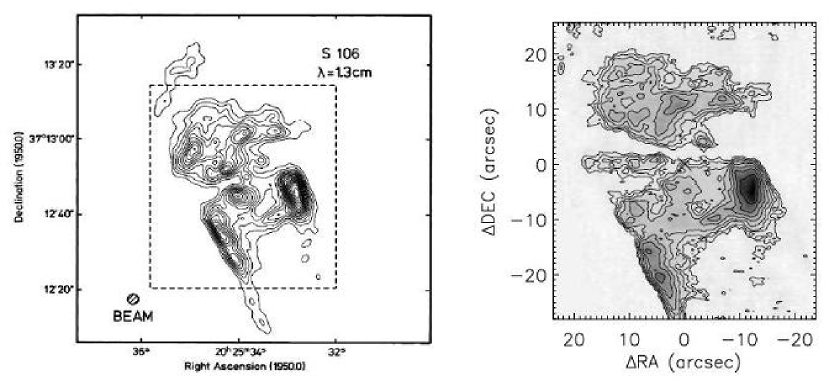
Figure 34: 1.3 cm continuum map (left, Felli et al., 1984, resolution$\sim 2.^{\prime\prime}3$) and integrated [Ne II] line flux map (right) of S106. Contours in the continuum map were drawn at each $5\%$ step from $5\%$ to $95\%$ of the peak value. The box drawn with dashed lines indicates the approximate area covered by the [Ne II] observations. Contours in the [Ne II] line map are drawn at $70\%$, $50\%$, $35\%$, $25\%$, $17.5\%$, $12.5\%$, $9\%$ and $6\%$ of the peak line emission. The spatial resolution of the radio map is $\sim 2.^{\prime\prime}3$. The (0,0) position is the location of a weak continuum source seen in the line observations. The peak [Ne II] surface brightness is 0.23 ergs cm^-2 s^-1 sr^-1. The total [Ne II] flux is 1.1$\times$10^-9 ergs cm^-2 s^-1.

S106 (G76.4 -0.6) is a well-known bipolar HII region consisting of two lobes with the symmetry axis oriented at a position angle of $\sim$30^∘. An equatorial gap is seen in all wavelengths from optical to radio. Earlier investigators suggest that a dense, circumstellar disk surrounds a star and blocks the ionizing photons in the disk plane forming a biconical nebula (Bally & Scoville, 1982). A point source, presumably the excitation source of the nebula, is located at the center of the equatorial gap (Pipher et al., 1976; Felli et al., 1984). Felli et al. (1984) noticed that the bright radio continuum peaks in S106 tended to be distributed at the edges of the radio lobes and inferred that the inner volume was filled with gas with lower density. A radio continuum map from their observations is shown in Figure 34. Dense molecular clumps were identified on both sides of the central source of the HII region (Schneider et al., 2002) but there is no evidence of a smooth molecular disk. Smith et al. (2001) imaged the region at 3 to 20 $\mu$m. Some of their images (11.7 $\mu$m) show two dark lanes. One crosses the center of the region from the east to the west and divides the region into the north and south lobes. The other originates east of the region, crosses the south lobe and forms a small angle ($\sim$30^∘) with the first dark lane.

The integrated [Ne II] line map and the radio continuum map are stunningly similar (Figure 34). The bipolar morphology and individual emission concentrations are clearly seen in both maps. The south lobe is characterized by a few bright clumps along the edge, while the north lobe contains more diffuse emission. The axis of the bipolar structure, which is indicated by the sharp edges of the south lobe, runs NNE-SSW. The main difference between the radio and [Ne II] maps is that the second dark lane seen in the infrared continuum is also seen in [Ne II].

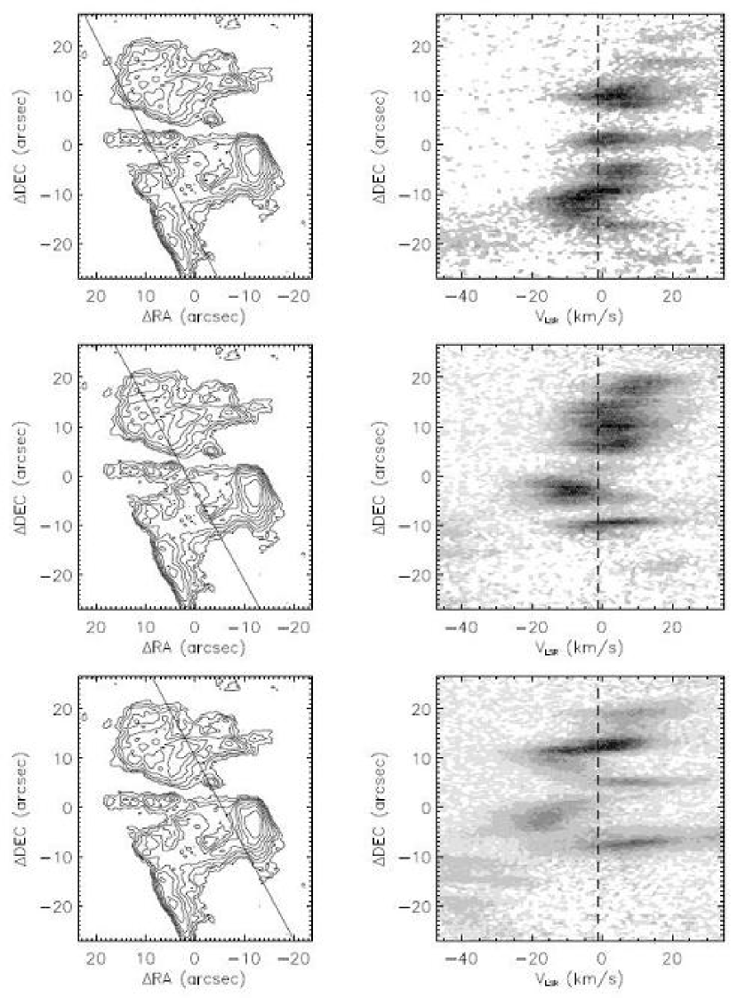
Figure 35: Position-velocity diagrams of S106 [Ne II] line observations. Contours in [Ne II] line flux maps are drawn at $70\%$, $50\%$, $35\%$, $25\%$, $17.5\%$, $12.5\%$, $9\%$ and $6\%$ of peak values (0.23 ergs cm^-2 s^-1 sr^-1) in the maps. Dashed lines in p-v diagrams show the ambient molecular material velocity.

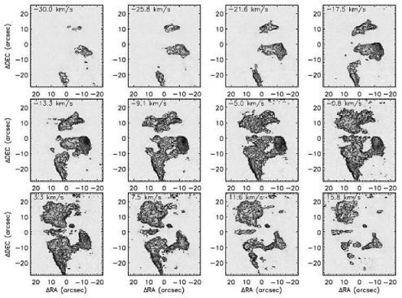
Figure 36: Channel maps of S106 [Ne II] line observations. Contours are drawn at $70\%$, $50\%$, $35\%$, $25\%$, $17.5\%$, $12.5\%$, $9\%$ and $6\%$ of the peak value of all channels. The peak value is 3.6 ergs cm^-2 s^-1 sr^-1 (cm^-1)^-1. The molecular cloud velocity is V_LSR = -1 km s^-1.

The velocity structure shown in the p-v diagrams (Figure 35) and the channel maps (Figure 36) is consistent with a picture of S106 as a nearly edge-on bipolar nebula. Both figures indicate that the south lobe is slightly blue shifted ($\sim$3 km s^-1) with respect to the molecular cloud velocity while the material in the northern lobe is on-average red-shifted by $\sim$4 km s^-1. At the same time, individual intensity peaks show moderately narrow ($\sim$10 km s^-1 lines. Projection effects may lead to velocity shifts from one emission peak to its neighbors.

4.14 NGC7538A

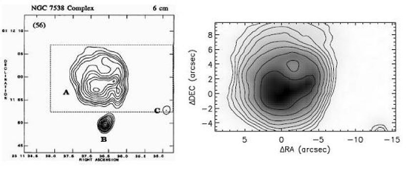
Figure 37: 6 cm continuum map (left, Wood & Churchwell, 1989b, restoring beam: $0.^{\prime\prime}38\times 0.^{\prime\prime}38$) and integrated [Ne II] line flux map (right) of NGC7538A. Contours in the continuum map were drawn at $95\%$, $90\%$, $80\%$, $70\%$, $60\%$, $50\%$, $40\%$ ,$30\%$, $20\%$, $15\%$, $10\%$, $5\%$, $-5\%$, $-10\%$, $-15\%$ and $-20\%$ of the peak value. The box drawn with dashed lines indicates approximately the area covered by the [Ne II] observations. Contours in the [Ne II] line map are drawn at $70\%$, $50\%$, $35\%$, $25\%$, $17.5\%$, $12.5\%$, $9\%$ and $6\%$ of the peak value in the map. The radio map has a synthesized beam with FWHM$\sim 0.^{\prime\prime}38\times 0.^{\prime\prime}38$. The (0,0) position is the location of the [Ne II] line emission peak. The peak [Ne II] surface brightness is 0.16 ergs cm^-2 s^-1 sr^-1. The total [Ne II] flux is 2.7$\times$10^-10 ergs cm^-2 s^-1.

NGC7538A belongs to an HII region-molecular cloud complex at a distance of ${\sim}3.5$ kpc (Hanson et al., 2002). In the 6 cm radio continuum image, it is a compact, spherical HII region with a radius $\sim 5^{\prime\prime}$ (Wood & Churchwell, 1989b) (Figure 37, left), corresponding to $\sim$19,000 AU. Molecular line observations show that molecular gas toward NGC7538 has a LSR velocity $-56.9$ km s^-1 (Dickel et al., 1981). Bloomer et al. (1998) suggested that NGC7538A is formed by a stellar wind bow shock with a star moving from the northwest to the southeast away from the Earth into the molecular cloud.

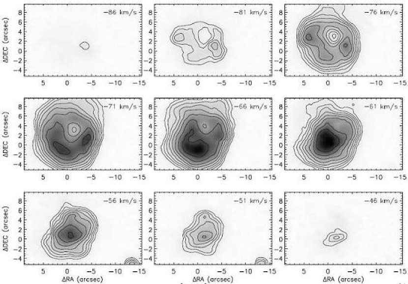
Figure 38: Channel maps of N7538 A [Ne II] line observations. Contours are drawn at $70\%$, $50\%$, $35\%$, $25\%$, $17.5\%$, $12.5\%$, $9\%$ and $6\%$ of the peak value of all channels. The peak value is 3.1 ergs cm^-2 s^-1 sr^-1 (cm^-1)^-1. The molecular cloud velocity is V_LSR = -57 km s^-1.

Since dust extinction toward the region is not huge ($A_{K}\sim 1.3$, Werner et al., 1979; Herter et al., 1981; Campbell & Thompson, 1984), our [Ne II] line map of NGC7538A (Figure 37, right) resembles the radio continuum map closely except that the radio component which should be at the southwestern corner of the source A, $\sim$(-5,-2), is not present in our [Ne II] map. This is probably due to our poor spatial resolution. [Ne II] line channel maps, spanning a velocity range from -82 to -51 km s^-1, are shown in Figure 38. A cavity can be seen in the most blue-shifted channels and in the integrated line map. The shape of the region changes from ring-like at the blue-shifted channels to core-like at the red-shifted channels. The channel maps in Figure 38 show that most of the ionized gas in NGC7538A is blue-shifted with respect to the molecular cloud. The limb-brightened appearance of the source in the integrated line strength and radio continuum maps (Figure 37) might lead to the conclusion that the source is a limb-brightened spherical shell. However, the pattern of a small central source at the molecular cloud velocity and a larger, shell-like structure at bluer velocities, combined with the “$\Lambda$” and “7” structures seen in the pv cuts through the source (Figure 39) argue against this picture. The kinematics and morphology are more consistent with a tangential flow along a shell with the symmetry axis close to the line of sight and with the vertex pointing away from the observer.

4.15 W3A+B

W3 belongs to an extensive HII region-molecular cloud complex located in the Perseus spiral arm (D = 2.0 kpc, Hachisuka et al., 2006). Aperture synthesis observations identified four compact/ultracompact radio continuum sources in a 3 arc minute diameter region (A-D, Wynn-Williams, 1971). Infrared imaging at 1.65 to 20$\mu$m revealed nine objects (IRS 1-9) in W3 (Wynn-Williams et al., 1972), four of which are associated with the compact radio continuum sources: IRS1 and IRS2 with the circular source W3A; IRS3 with W3B and IRS4 with W3C. Earlier authors have used the “broken-shell” morphology and the small velocity gradients seen in hydrogen recombination lines toward W3A to argue for a picture of this region as a blister flow (Dickel et al., 1983; Tieftrunk et al., 1997). W3B has also been characterized as an emerging blister flow (Tieftrunk et al., 1997).

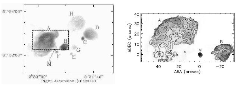
Figure 40: Grey-scale map of the radio 6 cm free-free continuum of W3 core (left) (Tieftrunk et al., 1997). The observations have a FWHM beam with a size of $0.^{\prime\prime}71\times 0.^{\prime\prime}56$. The flux in the region ranges from 0.1 mJy to 40 mJy beam^-1. The box drawn with dashed lines indicates the approximate area covered by our [Ne II] observations. Integrated [Ne II] line flux map of W3 A and B region (right). The (0,0) position is the peak location of integrated emission map. Contours are drawn at $70\%$, $50\%$, $35\%$, $25\%$, $17.5\%$, $12.5\%$, $9\%$ and $6\%$ of the peak value. The peak [Ne II] surface brightness is 0.26 ergs cm^-2 s^-1 sr^-1. The total [Ne II] flux from W3A is 1.3$\times$10^-9 ergs cm^-2 s^-1. The total [Ne II] flux from W3B is 3.7$\times$10^-10 ergs cm^-2 s^-1.

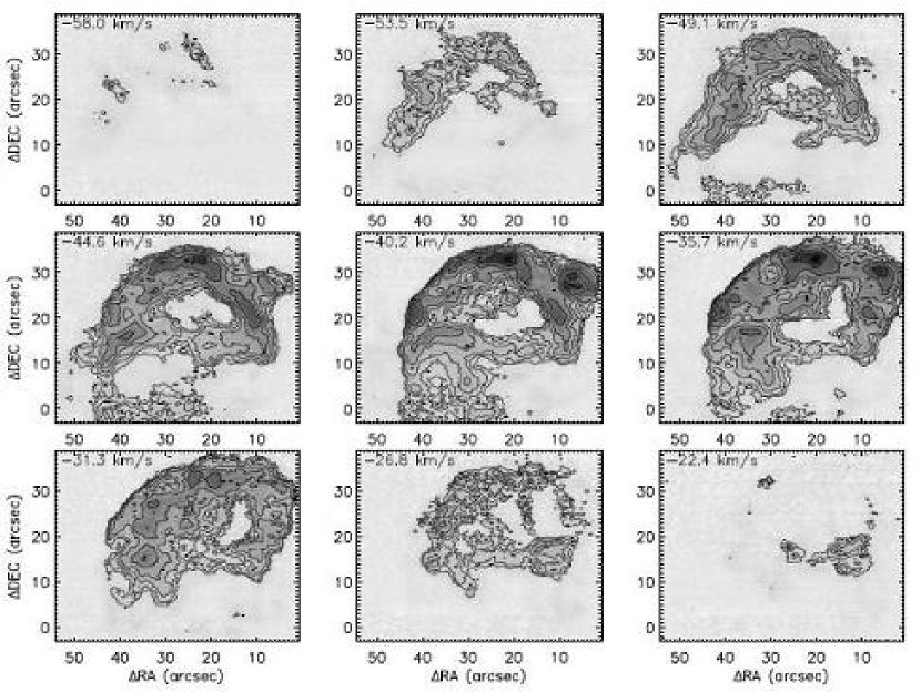
Figure 41: Channel maps of W3 A [Ne II] line observations. Contours are drawn at $70\%$, $50\%$, $35\%$, $25\%$, $17.5\%$, $12.5\%$, $9\%$ and $6\%$ of the peak value of all channels. The peak value is 2.8 ergs cm^-2 s^-1 sr^-1 (cm^-1)^-1. The molecular cloud velocity is V_LSR = -40 km s^-1.

W3A has the morphology of a limb-brightened broken shell in our [Ne II] map (Figure 40), in close agreement with the distribution of the radio continuum emission. Most of the line emission forms a crescent open to the south with a horizontal structure crossing the center of the incomplete shell. An irregular emission cavity is present inside the crescent. Two finger-like structures extend from the southeast corner of the ring to the south. If we ignore these finger-like structures and another small lobe of emission on the northwest edge of the shell, the region closely resembles a half-ring. Such an image becomes clear in the channel maps of the region (Figure 41). The half-ring morphology is present in channels over a broad velocity range. The sharp outer edge of the ring is evident. The emission level drops rapidly to the background level within a few arcseconds.

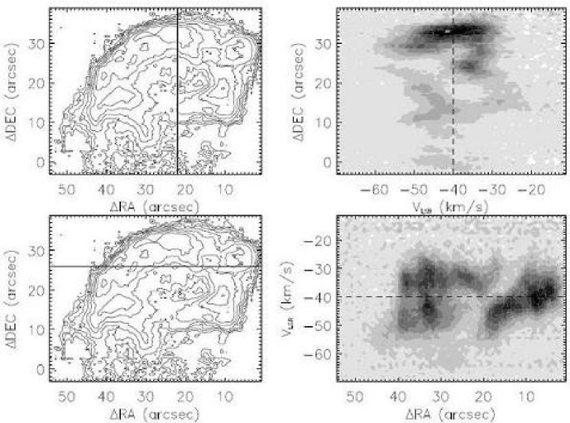
Figure 42: Position-velocity diagrams of W3 A line observations. Contours in line flux maps are drawn at $70\%$, $50\%$, $35\%$, $25\%$, $17.5\%$, $12.5\%$, $9\%$ and $6\%$ of peak values (0.13 ergs cm^-2 s^-1 sr^-1) of the maps. Dashed lines in p-v diagrams show the ambient molecular material velocity.

The shell-like morphology of W3A might lead one to expect the source to have the kinematics of an expanding shell. However, p-v diagrams (Figure 42) of the region do not support this picture. We do not see the two components toward the center of the source which, in an expanding shell, would arise from the front and back sides of the shell and would gradually merge into one component at an intermediate velocity at the edge of the shell. Instead, we see a very broad line ($\geq$25 km s^-1) along the bright arc-like rim of the region becoming narrow blue-shifted and red-shifted lines toward the center of the region. The change of the line width and the center velocities of the lines are abrupt. A surface flow, rather than an expanding shell, can better explain the observed p-v structure. The fact that both p-v cuts show the same pattern of a broad feature at the bright limb followed by a double line within the cavity implies that the vertex of the flow lies between the two cuts. An examination of the -53.5 km s^-1 and -26.8 km s^-1 channel maps in Figure 41 supports this picture. The emission in the southern part of W3A comes from a narrower velocity range and therefore is not part of the surface flow seen in the north.

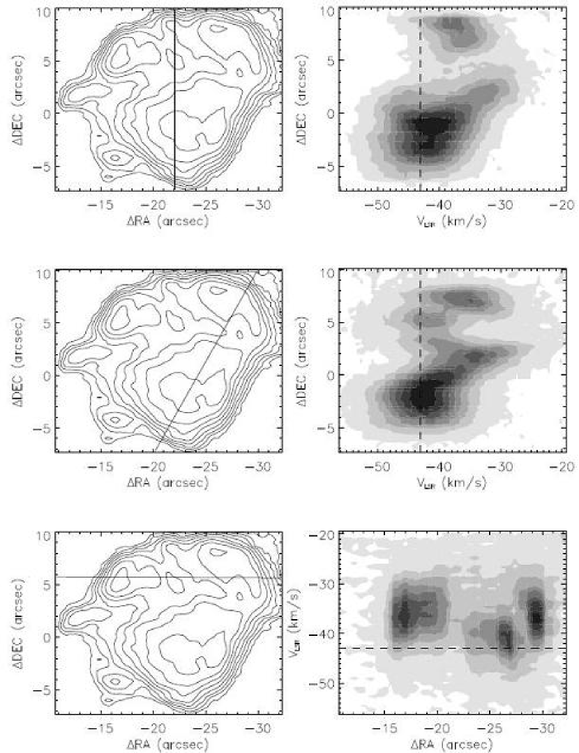
Figure 43: Position-velocity diagrams of W3 B line observations. Contours in line flux maps are drawn at $70\%$, $50\%$, $35\%$, $25\%$, $17.5\%$, $12.5\%$, $9\%$ and $6\%$ of peak values (0.17 ergs cm^-2 s^-1 sr^-1) of the maps.

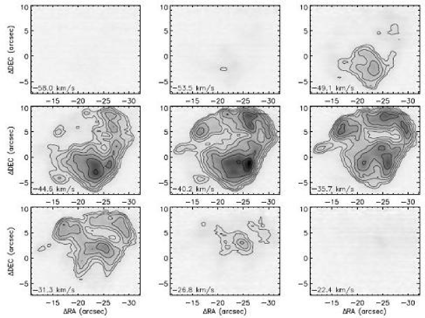
Figure 44: Channel maps of W3 B [Ne II] line observations. Contours are drawn at $70\%$, $50\%$, $35\%$, $25\%$, $17.5\%$, $12.5\%$, $9\%$ and $6\%$ of the peak value of all channels. The peak value is 5.2 ergs cm^-2 s^-1 sr^-1 (cm^-1)^-1. The molecular cloud velocity is V_LSR = -43 km s^-1.

The compact HII regions W3B and W3A have similar central velocities and line widths. The overall [Ne II] line emission distribution in W3B (see left panels in Figure 43) looks like an irregular shell. The line profile at most positions in the region can be fit by a single Gaussian. W3B contains a low surface brightness cavity, which can be seen in both the integrated line map and the channel maps (Figure 44) of the region. The total shift in velocity centroid in W3B is relatively modest, from $\sim$-42 km s^-1 to -34 km s^-1 and there is an apparently random element to the velocity variations at the 2-3 km s^-1 level. Nonetheless, both the channel maps (Figure 44) and the p-v cuts (Figure 43) are consistent with tangential flow along the ionized walls of a cavity. The channel maps show emission from the central region primarily at the least negative velocities, while the shell is most prominent in the bluer channels. The p-v diagrams also show the reddest velocities at positions crossing the center of the cavity and the bluest velocities along the edge.

5 Discussion

We have presented high spatial and spectral resolution mapping of the 12.8 $\mu$m [Ne II] line toward a sample of 18 compact and ultracompact HII regions, where we count distinct HII regions within clusters as separate sources. In our discussion, we make use of previously published results for two of the 18 regions: G29.96-0.02 (Zhu et al., 2005) and W51 IRS2 (Lacy et al., 2007). We also include in the discussion one source (Mon R2, Jaffe et al., 2003), for which no results are presented in the current paper, bringing our sample to 19 sources.

In order to discuss possible interpretations of the observed source morphologies and kinematics, we first sketch p-v diagrams of several types of models that have been suggested for UCHII regions. We then compare the observed morphologies and kinematics to these sketches. We emphasize that the sketches are only meant to be qualitative descriptions of generic models. They are not derived from hydrodynamic simulations.

5.1 Qualitative Models

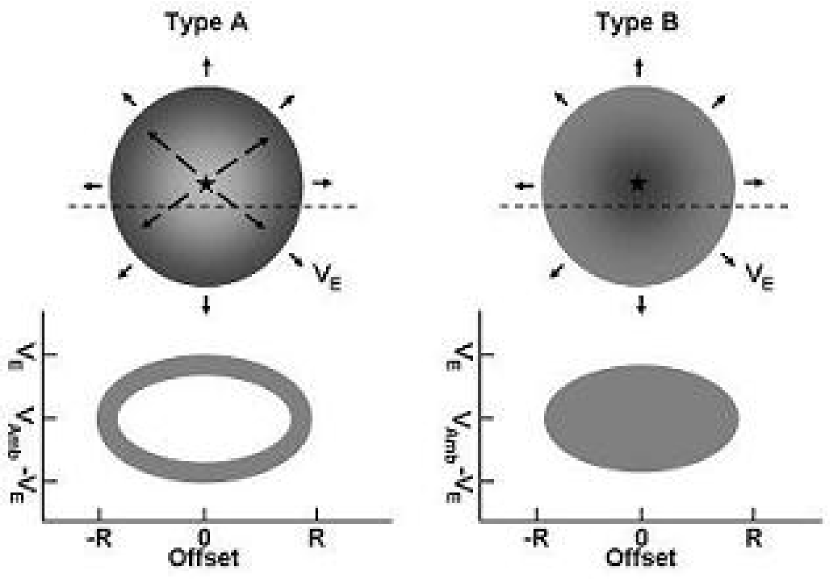
Figure 45: Sketches of position-velocity diagrams of an expanding shell-like HII region (left) and an expanding spherical HII region (right). The expansion speed is V_E. The molecular cloud velocity is V_amb. The dashed lines show the locations of the p-v cuts. The solid arrows in the morphology diagrams indicate the moving directions of ionized gas relative to ambient molecular material and the dashed arrows show the moving directions of stellar wind material with respect to the central stars.

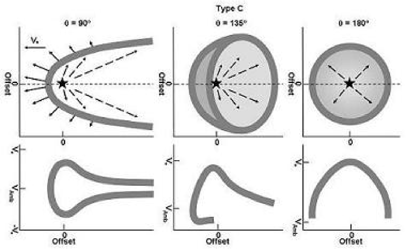
Figure 46: Sketches of position-velocity diagrams of a stellar wind bow shock HII region at three different viewing angles. Note that the velocity vectors are shown in the frame of reference of the ambient molecular cloud; the shell is not expanding in the moving frame of reference of the star. The molecular cloud velocity is V_amb and the ionizing star is moving supersonically at a speed of V_⋆ relative to the molecular cloud. The ram pressures of incoming cloud material and stellar wind material confine the ionized material in a compressed shell which moves with the star in the cloud. The dashed lines show the locations of the p-v cuts. The p-v diagrams in the middle and right panels are drawn for stars moving away from the observer ($\theta>90^{\circ}$). The p-v diagrams would be mirrored about V_amb for stellar motions toward the observer ($\theta<90^{\circ}$).

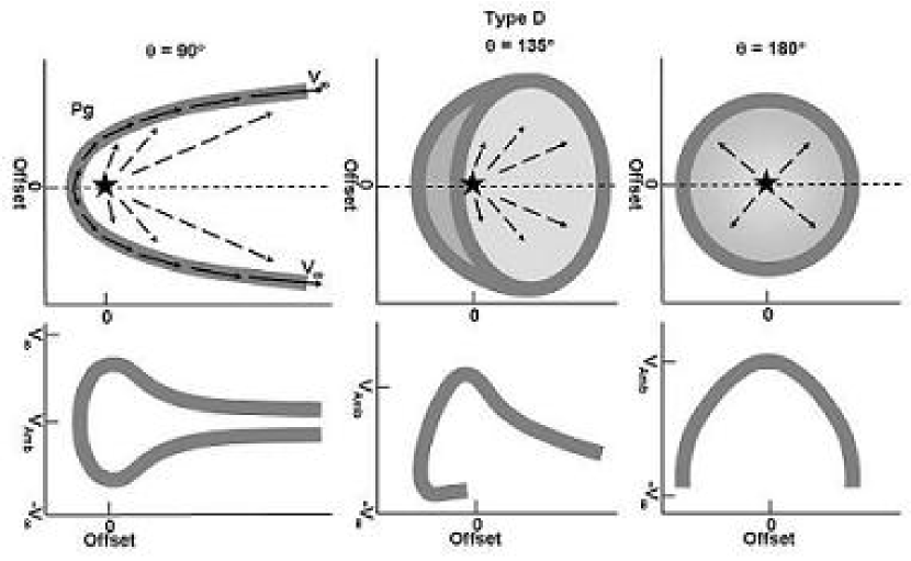
Figure 47: Sketches of position-velocity diagrams of a stellar wind pressure-driven HII region at three different viewing angles. The molecular cloud velocity is V_amb and the star with a stellar wind is stationary with the cloud. The ionized gas is compressed by the stellar wind into a shell and moves along the shell under the influences of the density gradient and the stellar wind pressure. V_∞ is the exiting speed of the ionized gas. The dashed lines show the locations of the p-v cuts. The p-v diagrams are similar to those in Fig. 46, but are offset toward negative V_LSR for the head of the shell tipped away from the observer ($\theta>90^{\circ}$). The p-v diagrams would be mirrored about V_amb for stellar motions toward the observer ($\theta<90^{\circ}$).

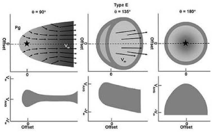
Figure 48: Sketches of position-velocity diagrams of a blister flow HII region at three different viewing angles. The molecular cloud velocity is V_amb and the star is stationary. No stellar wind is present. The cloud material is continually evaporated by the stellar radiation and forced by pressures to flow along the density gradient. The V_∞ is the exiting speed of the ionized gas. The dashed lines show the locations of the p-v cuts. The figures show p-v diagrams of the region when the head of the region is tipped away from the observer ($\theta>90^{\circ}$). The p-v diagrams would be mirrored about V_amb for stellar motions toward the observer ($\theta<90^{\circ}$).

To facilitate the discussion of the observed gas motions, we first consider qualitative kinematic models of UCHII regions. Sketches of several types of models of UCHII regions are shown in Figures 45-48.

A. (Figure 45) An uniformly expanding shell source appears as a limb-brightened disk. Its p-v diagram is ring-like, centered on the molecular cloud velocity, V_amb.

B. (Figure 45) An expanding filled sphere appears as a limb-darkened disk. Its p-v diagram is a filled ellipse centered at V_amb.

C. (Figure 46) The appearance of a bow-shock source, in which a wind from a star moving supersonically through a molecular cloud sweeps up a paraboloidal shell, with the motion of the gas in the shell resulting from the combined momenta of the stellar wind and the swept-up material (Mac Low et al., 1991; van Buren & Mac Low, 1992; Wilkin, 2000; Zhu et al., 2005; Arthur & Hoare, 2006) depends on the viewing angle. If viewed from the side ($\theta=90^{\circ}$, left panel), two velocities are seen at each offset, on opposite sides of V_amb. The line is broad in the head, and the two velocities approach each other in the tail. If viewed from the tail ($\theta=180^{\circ}$, right panel), the source would not be obviously cometary in appearance, and the velocity would vary from V_⋆ at the center to V_amb at the edges. From an intermediate angle ($\theta=135^{\circ}$, middle panel), we see a p-v pattern like those seen in G29.96, but offset in velocity. A broad line, centered between V_amb and V_⋆ is seen at the head of the comet. Of the two velocities seen at $\theta=90^{\circ}$, the V $<$ V_amb branch is foreshortened and may blend into the head (see Figure 4). The V $>$ V_amb branch rises toward V_⋆ then falls back toward V = V_amb. The line centroid is at V $>$ V_amb. The p-v diagrams would be mirrored about V_amb if the star were moving toward the observer ($\theta<90^{\circ}$).

D. (Figure 47) A paraboloidal shell can also occur in which the motion of the gas in the shell is predominantly due to the pressure gradient along the shell, which causes an acceleration of the gas toward the tail (Zhu et al., 2005; Arthur & Hoare, 2006). In this case, the paraboloidal shape of the shell could result either from a relatively slow motion of the star through the molecular cloud or from a density gradient in the cloud. The resulting appearance and p-v diagrams are similar to those of the bow-shock model, but the p-v diagrams are offset toward negative velocities, with the velocity centroid at V $<$ V_amb (for $\theta>90^{\circ}$). This is the offset seen in G29.96, indicating that it belongs to this category.

E. (Figure 48) A filled blister flow could result if the wind from the ionizing star is too weak to prevent the ionized gas from flowing away from the surface of the molecular cloud, past the star (Yorke et al., 1983; Comeron, 1997; Henney et al., 2005; Arthur & Hoare, 2006). Such a region is formed when a density gradient is present in the natal molecular cloud. In this case, the source morphology and p-v diagrams would depend on the shape of the blister cavity in the molecular cloud, but blister flows are largely axial and a broad line would be likely to be seen at all positions. For $\theta>90^{\circ}$, the line centroid is at V $<$ V_amb. The largest velocities would be seen toward the tail, or at the center for $\theta\approx 180^{\circ}$.

A number of sources in our sample either have confused kinematics or have kinematics for which we have no simple qualitative models: Several sources show ring, horseshoe, or bipolar morphologies, without the kinematic signatures of shells or paraboloidal flows. Several regions appear to be clusters of overlapping sources, making the interpretation of their kinematics difficult. Several sources have distinctly different morphologies in [Ne II] and the radio continuum, suggesting that variable extinction is distorting their appearance in the infrared. These sources also have confusing kinematics. And several sources are too small for their [Ne II] kinematics to have been resolved.

5.2 Observed Source Morphologies

The extraordinarily good match between the radio and [Ne II] morphologies in the majority (12 of 16) of the resolved sources indicates that most neon is in Ne⁺, that the gas density is almost everywhere below the critical density of the 12.8 $\mu$m line, and that the centimeter-wave radio continuum emission is for the most part optically thin. Extinction is the most likely cause of the strong differences between radio continuum and [Ne II] morphologies in the other four sources. Some of the differences could also be due to incomplete UV coverage in the radio snapshot observations. And, differences in sensitivity between [NeII] and radio continuum observations may also play a role.

In many cases, radio interferometer observations show that UCHII regions are accompanied by substantial radio continuum flux from extended, low-surface brightness ionized gas (Kurtz et al., 1999; Kim & Koo, 2001). These results imply that UCHII regions may exist in asymmetric regions where the ionizing radiation reaches dense gas in one direction and more extended low density gas in the other direction. Our scanning technique does not permit us to find these extended haloes in [Ne II] due to limited sky area we can cover and the sky background subtraction method we use, but the frequent presence of emission halos may have implications for the interpretation of the source kinematics.

5.3 Observed Source Kinematics

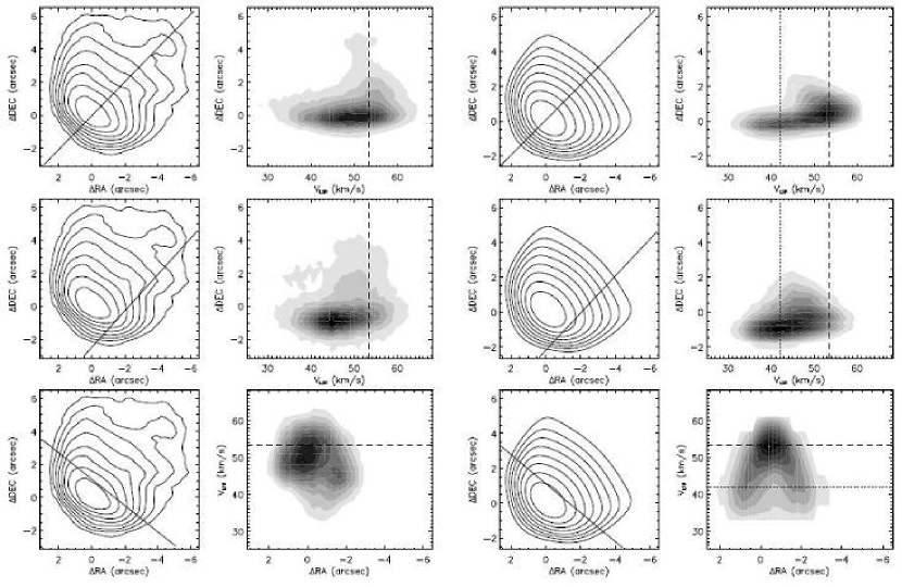
Figure 17: Position-velocity diagrams of [Ne II] line observations (two columns on the left) and a bow shock model (two columns on the right) of G43.89 -0.78. Contours in line flux maps are drawn at $70\%$, $50\%$, $35\%$, $25\%$, $17.5\%$, $12.5\%$, $9\%$ and $6\%$ of the peak values (0.22 ergs cm^-2 s^-1 sr^-1) in the maps. See text for a description of the model. The dashed lines in the p-v diagrams show the ambient molecular cloud velocity. Dotted lines in the model p-v diagrams show the ambient material velocity in the model.

Of the 12 sources that are resolved and not badly confused by extinction, nine show clear evidence of bulk motions, which are usually not symmetric about the molecular cloud velocities. These nine sources all show strong evidence of tangential flows along the surfaces of shells. Three of these sources, G29.96 (Figures 3 and 4), G33.92 (Figure 13), and G43.89 (Figure 17), show, with varying degrees of clarity, the “$\Lambda$” and “7” patterns in p-v diagrams that are similar to the patterns established in the surface flow models (types C and D). In these three cases, the patterns indicate that the terminal velocities are blueshifted with respect to the molecular cloud velocities. Along the symmetry axis, the velocities cross the molecular cloud velocity from blue to red and back to blue going from the vertex into the source for G29.96 and G33.92. In G43.89, the velocity approaches the cloud velocity from the blue side but does not cross it before moving back to the blue. The kinematic behavior we observe in all three sources is very similar to what we see in the models of G29.96 (Figures 3 and 4), which are tilted with the vertex away from the observer and have an inclination of the symmetry axis of about 45^∘ with respect to the line of sight. With their vertices pointed away from the observer, the blueshift relative to V_amb means that these sources are of kinematic type D (pressure-driven surface flows; Figure 47).

The three sources in our sample whose [Ne II] and radio continuum morphologies most closely resemble limb-brightened spherical shells do not have kinematic patterns consistent with a closed-shell geometry. The kinematic patterns for three of the sources, NGC 7538A (Figure 39), W3B (Figure 43), and W51 IRS2, (see Lacy et al., 2007), are consistent with motion of the ionized gas along roughly parabolic shells with vertices pointing almost directly away from the observer. In the position-velocity plots, the most positive velocities, usually close to the velocity of the dense molecular gas, are toward the vertex while the velocities along the bright rim are shifted to the blue. The presence of this pattern is largely independent of the position angle of the position-velocity cut through the center of the source. These sources are of kinematic type D with $\theta\approx 180^{\circ}$.

The remaining sources with understandable kinematics also have a strongly limb-brightened appearance. The kinematics revealed by the [Ne II] spectroscopy show that G30.54 (Figure 11), W3A (Figure 42), and Mon R2 (Jaffe et al., 2003) are also likely to be limb-brightened parabolas with significant flow of the ionized gas along the ionized shell. For these three sources, however, the kinematics indicate that the symmetry axes lie near the plane of the sky. The sources show broad lines at the source vertex and then double lines farther along the symmetry axis with the two components appearing at the extreme velocities of the line seen at the vertex. Along the edges of each source, the lines are single and significantly narrower. These sources are of either kinematic type D or type C, with $\theta\approx 90^{\circ}$.

Four sources have very similar [Ne II] and radio morphologies, but do not fit into any of the kinematic categories we have discussed. S106 (Figure 34) has a clear bipolar morphology, but confused kinematics. G45.12N (Figure 21) has a cometary morphology, but does not have obvious cometary kinematics, of either type C or type D. G45.12SW (Figure 22) has a ring or shell morphology, but does not have the kinematic signature of a shell. K3-50A (Figure 31) appears to be a cluster of sources, which are too blended to allow us to sort out their kinematics. The peaks in the IRTF map of [Ne II] in W51 IRS2 (Figure 25) are also blended. The Gemini map of Lacy et al. (2007) separates these sources but does not resolve their kinematics. However, the kinematics of the extended ionized gas in W51 IRS2 shown in Lacy et al. (2007) look much like a type D surface flow with $\theta\approx 180^{\circ}$.

Complex morphologies and kinematics in the four sources with substantially different [Ne II] and radio continuum morphologies prevent a coherent explanation for gas motion in these sources. However, it is clear that systematic gas motions are present. In G11.94, there is a component of the [Ne II] emission at the same velocity as the ambient cloud (Figure 8), but there is also a substantial amount of emission at many positions in a red wing or in an identifiable red component. In G45.45 (Figure 23), the kinematic pattern is confusing, and the most prominent feature in [Ne II] is not apparent in the radio continuum. G61.48 (Figure 29) is the source where the [Ne II] morphology least resembles the distribution of the radio continuum emission. The [Ne II] emission we see may therefore not be sampling the bulk of the gas, but the dominance of red-shifted gas in the RRL observations (Garay et al., 1994) is consistent with the conclusion from the [Ne II]-radio continuum morphology difference, namely that the source is on the back side of the molecular cloud and the ionized material is flowing away from the neutral core.

5.4 Comparison of Observed Sources with Qualitative Models

The kinematic types that we have assigned to observed sources are given in Table 2. Examination of this list shows that none of the observed sources fits into category A or B, the classical expanding shell and sphere models of HII regions. None has a ring-like p-v diagram of an expanding shell, and the sources with broad lines are either too small for their morphologies to be apparent or have confused morphologies. In addition, none of the sources fits into category E, the classical filled blister flow with the ionized gas flowing away from the ionization front.

Even more remarkably, in spite of the frequency of bow-shock morphologies, none of the observed sources clearly fits into category C, a bow shock moving with a star through a molecular cloud. Because they are nearly edge-on, Mon R2, G30.54, and W3A could fit into either category C or category D. The other sources with cometary kinematic signatures all have p-v patterns characteristic of sources tipped away from the observer (${\theta}>90^{\circ}$) with their velocity centroids blueshifted relative to the neighboring molecular material, the signature of a pressure-driven surface flow.

The preponderance of sources with their tails tipped toward the observer ($\theta\geq 90^{\circ}$) probably results from a combination of extinction and selection effects. The extinction at 12.8 $\mu$m is relatively low (A_12.8/A_V$\sim$0.05, Rieke & Lebofsky, 1985; Rosenthal et al., 2000), but the column density through the kind of massive core that harbors massive young stars and UCHII regions can be substantial (A_V $\approx$ a few hundred, Beuther et al., 2000). The density in such cores drops rather steeply, with power-law exponents of 1.6-1.8 (Mueller et al., 2002; Beuther et al., 2002). If UCHII regions are not in the centers of cores, they should therefore be visible in [Ne II] when the exciting stars lie between the front side and $\theta\approx 90^{\circ}$. Our survey was somewhat biased in favor of sources lying on the front sides of molecular clouds by including sources known from optical and near-infrared observations (NGC 7538, W3, and Mon R2). In addition, we were forced to abandon efforts to observe several UCHII regions (G8.67-0.36, G10.10+0.74, G10.62-0.38, G12.208-0.10, G33.50+0.20, G42.42-0.27, G45.47+0.05, G50.23+0.33) because they were undetectable or too faint to map. These selection effects are likely to explain the lack of sources with kinematics indicating that they lie on the back sides of their clouds.

More than half of the observed sources fit into category D, a flow along the surface of a paraboloidal shell, which accelerates relative to molecular cloud as it moves away from the apex of the paraboloid. Although we have not made a hydrodynamic model of such a flow, we know of no driving mechanism for the acceleration other than the pressure gradient in the ionized gas. Zhu et al. (2005) found that the pressure gradient acceleration would be small if the ionized and swept-up molecular gas were coupled so both had to be accelerated. But we have estimated the acceleration if the ionized gas is allowed to slip past the molecular shell, and we find that speeds $\sim$20-30 km s^-1 can occur. The hydrodynamic models of Arthur & Hoare (2006) include the essential effects present in the combination of blister and bow shock models: density gradients in the neutral medium, stellar winds, and stellar motion. The Arthur & Hoare (2006) models do an excellent job of matching the range of source morphologies and reproduce the most significant kinematic signatures using reasonable values for density gradients, mass loss rates, and stellar velocities. One critical area where they fall short is in explaining the width of the lines at the source vertex. The observed effect is most evident in W3A (Figure 42) and in Mon R2 (Jaffe et al., 2003) where the symmetry axes are near the plane of the sky. The splitting of the broad line into two narrow lines at the velocity extremes of the broad line as one crosses the shell to the inside implies that the gas accelerates to $\sim~{}\pm$10 km s^-1 within a small solid angle (less than a steradian, as seen from the point of view of the ionizing star) at the vertex. This, in turn, implies a significant pressure gradient.

The [Ne II] kinematics of our sample unite a large and diverse group of UCHII and compact HII regions into a single empirical picture: The HII regions coexist with dense and massive molecular cores (Beuther et al., 2002; Shirley et al., 2003; Sridharan et al., 2002). The ionized regions have the form of partial, roughly parabolic shells with their open sides usually pointing away from the centers of the dense neutral condensations and gas flows tangentially along these shells.

The evidence that very many UCHII regions are dense shells with tangential flows away from the parent molecular cores has implications for the survivability of the molecular cores. Earlier examinations of the erosion of dense cores by external O stars did not take the compression of neutral material by stellar wind shocks into account. These efforts led to estimates that when as little as 4% of the core material formed into stars with a Salpeter IMF, these stars could erode the remaining core entirely away (Whitworth, 1979). It has already been pointed out, however that the dense shells formed by stellar wind pressure would greatly inhibit the process of erosion (Churchwell, 1991; Lumsden & Hoare, 1999; Hoare, 2006). Our results indicate that most if not all OB stars breaking out of dense cores form such dense shells at their boundaries.

Figure 39: Position-velocity diagrams of NGC7538 A [Ne II] line observations. Contours in line flux maps are drawn at $70\%$, $50\%$, $35\%$, $25\%$, $17.5\%$, $12.5\%$, $9\%$ and $6\%$ of the peak values (0.16 ergs cm^-2 s^-1 sr^-1) of the maps. Dashed lines in p-v diagrams show the ambient molecular material velocity.

Table 1: OBSERVATIONAL DATA

Object	Date	RA(J2000.0)	DEC	d	VLSR	SW	SL	STS	PS	ME	IT
	mm/dd/yy	hh mm ss.sss	dd mm ss.sss	(kpc)	(km s-1)	(′′)	(′′)	(′′)	(′′)	(′′ $\times$ ′′)	(sec)
2G5.89 -0.39	06/11/03	18 00 30.4	-24 04 00	2.6	9	0.9	10.8	0.4	0.360	6${\times}$6	180
1G11.94 -0.62	07/02/03	18 14 02.2	-18 53 26	4.2	39	1.4	10.8	0.7	0.360	18${\times}$16	12
2G29.96 -0.02	06/11/01	18 46 03.9	-02 39 22	7.4	98	0.9	10.8	0.4	0.360	20.4${\times}$13	16
2G30.54 +0.02	06/30/03	18 46 59.5	-02 07 26	13.8	48	1.4	10.8	0.7	0.360	12${\times}$12	16
2G33.92 +0.11	06/11/01	18 52 50.2	00 55 29	8.3	108	0.9	10.8	0.4	0.360	17${\times}$15	50
2G43.89 -0.78	07/01/03	19 14 26.2	09 22 34	4.2	53.5	1.4	10.8	0.7	0.360	12${\times}$12	16
2G45.07 +0.13	07/01/03	19 13 22.1	10 50 53	6.0	59	1.4	10.8	0.7	0.360	7${\times}$8	12
2G45.12 +0.13	07/01/03	19 13 27.8	10 53 36	6.9	59	1.4	10.8	0.7	0.360	15${\times}$18	16
2G45.45 +0.06	06/11/01	19 14 21.4	11 09 14	6.6	59.5	0.9	10.8	0.4	0.360	15${\times}$12	52
1W51 IRS2	06/30/03	19 23 39.9	14 31 09	6.6	58.3	1.4	10.8	0.7	0.360	30${\times}$14	12
1G61.48 +0.09B	07/01/03	19 46 49.2	25 12 43	5.4	22	1.4	10.8	0.7	0.360	60${\times}$19	16
1K3-50A	06/30/03	20 01 45.7	33 32 43	8.7	-24.4	1.4	10.8	0.7	0.360	12${\times}$12	24
1S106	06/29/03	20 27 26.8	37 22 48	0.6	-1.0	1.4	10.8	0.7	0.360	47${\times}$53	16
1NGC7538A	09/13/02	23 13 45.6	61 28 18	3.5	-56.9	1.4	10.1	1.0	0.360	29.4${\times}$16.2	$\geq$20
1W3A	07/01/03	02 25 40.8	62 05 53	2.0	-40	1.4	10.8	0.7	0.360	86${\times}$37	$>$8
1W3B	07/03/03	02 25 36.9	62 05 45	2.0	-43	1.4	10.8	0.7	0.360	61${\times}$44	$>$8

Note. — The observational parameters (SW: slit width, SL: slit length, STS: step size, PS: plate scale, ME: map extent, IT: pixel integration time) of observations. The shown coordinates are for the (0,0) positions in [Ne II] line maps. Two methods are used in determining these coordinates: ¹ Read from published figures. Both qualities of the figures and the reading process can affect uncertainties of the resulting coordinates, which can be over 1^′′. ² Cross-correlate [Ne II] line maps resampled on fine grids (pixel size $\leq$0.1^′′) and available radio continuum maps to find the best morphological fit. Uncertainties of these coordinates should be better than 0.5^′′. Nasa/IPAC Extragalactic Database (NED) coordinate calculator is used to convert obtained B1950.0 coordinates to J2000.0 coordinates. ^a Kim & Koo (2003); ^b Hatchell et al. (1998); ^c Churchwell et al. (1990); ^d Wood & Churchwell (1989b); ^e Shepherd & Churchwell (1996); ^f Harris (1975); ^g Staude et al. (1982); ^h Schneider et al. (2002); ⁱ Hanson et al. (2002) ^j Dickel et al. (1981); ^k Hachisuka et al. (2006); ^l only for W3A, Kantharia et al. (1998); ^m only for W3B, Tieftrunk et al. (1995)

Table 2: OBSERVED KINEMATIC TYPES

Object	Type	Comments
Mon R2	C/D	70∘ viewing angle, see Zhu et al. (2005)
G5.89 -0.39	?	barely resolved
G11.94 -0.62	?	multiple peaks, extinction lanes, complex kinematics, $\bar{V}\approx V_{amb}$
G29.96 -0.02	D	140∘ viewing angle, see Zhu et al. (2005)
G30.54 +0.02	C/D?	horseshoe morphology, weak type D signature on axis
G33.92 +0.11	D	confused morphology, but clear kinematic signature
G43.89 -0.78	D	clear type D morphology and kinematics
G45.07 +0.13	?	unresolved, 1′′ diameter
G45.12 +0.13N	?	appears cometary but without obvious cometary kinematics
G45.12 +0.13SE	?	barely resolved
G45.12 +0.13SW	?	broken ring, multiple peaks
G45.45 +0.06	?	confused line morphology, with different [Ne II] and ff morphologies
W51 IRS2	D	[S IV] has $\theta\approx 180^{\circ}$, type D kinematics (Lacy et al., 2007),
		[Ne II] shows superimposed sources
G61.48 +0.09B	?	extinction lanes, complex line morphology and kinematics, $\bar{V}>V_{molec}$
K3-50A	?	three blended peaks, extended line emission
S106	?	bipolar, with unclear kinematics
NGC7538A	D	shell-like appearance, tail-on type D kinematics
W3A	C/D	cometary with $\theta\approx 90^{\circ}$
W3B	D?	shell-like appearance, confusing kinematics

Note. — Kinematic types: A. expanding shell, B. expanding sphere, C. bow shock from moving star, D. pressure-driven surface flow, E. blister.

References

- Acord et al. (1998) Acord, J. M., Churchwell, E., & Wood, D. O. S. 1998, ApJ, 495, L107+
- Arthur & Hoare (2006) Arthur, S. J. & Hoare, M. G. 2006, ApJS, 165, 283
- Ball et al. (1992) Ball, R., Arens, J. F., Jernigan, J. G., Keto, E., & Meixner, M. M. 1992, ApJ, 389, 616
- Bally & Scoville (1982) Bally, J. & Scoville, N. Z. 1982, ApJ, 255, 497
- Beuther et al. (2000) Beuther, H., Kramer, C., Deiss, B., & Stutzki, J. 2000, A&A, 362, 1109
- Beuther et al. (2002) Beuther, H., Schilke, P., Menten, K. M., Motte, F., Sridharan, T. K., & Wyrowski, F. 2002, ApJ, 566, 945
- Bloomer et al. (1998) Bloomer, J. D., Watson, D. M., Pipher, J. L., Forrest, W. J., Ali, B., Greenhouse, M. A., Satyapal, S., Smith, H. A., Fischer, J., & Woodward, C. E. 1998, ApJ, 506, 727
- Campbell & Thompson (1984) Campbell, B. & Thompson, R. I. 1984, ApJ, 279, 650
- Churchwell (1991) Churchwell, E. 1991, in NATO ASIC Proc. 342: The Physics of Star Formation and Early Stellar Evolution, ed. C. J. Lada & N. D. Kylafis, 221–+
- Churchwell (1999) Churchwell, E. 1999, in NATO ASIC Proc. 540: The Origin of Stars and Planetary Systems, ed. C. J. Lada & N. D. Kylafis, 515
- Churchwell (2002) Churchwell, E. 2002, ARA&A, 40, 27
- Churchwell et al. (1990) Churchwell, E., Walmsley, C. M., & Cesaroni, R. 1990, A&AS, 83, 119
- Comeron (1997) Comeron, F. 1997, A&A, 326, 1195
- Crowther & Conti (2003) Crowther, P. A. & Conti, P. S. 2003, MNRAS, 343, 143
- De Buizer et al. (2003) De Buizer, J. M., Radomski, J. T., Telesco, C. M., & Piña, R. K. 2003, ApJ, 598, 1127
- de Pree et al. (1994) de Pree, C. G., Goss, W. M., Palmer, P., & Rubin, R. H. 1994, ApJ, 428, 670
- de Pree et al. (2005) de Pree, C. G., Wilner, D. J., Deblasio, J., Mercer, A. J., & Davis, L. E. 2005, ApJ, 624, L101
- Dickel et al. (1981) Dickel, H. R., Dickel, J. R., & Wilson, W. J. 1981, ApJ, 250, L43
- Dickel et al. (1983) Dickel, H. R., Harten, R. H., & Gull, T. R. 1983, A&A, 125, 320
- Dopita et al. (2006) Dopita, M. A., Fischera, J., Crowley, O., Sutherland, R. S., Christiansen, J., Tuffs, R. J., Popescu, C. C., Groves, B. A., & Kewley, L. J. 2006, ApJ, 639, 788
- Downes et al. (1980) Downes, D., Wilson, T. L., Bieging, J., & Wink, J. 1980, A&AS, 40, 379
- Dyson et al. (1995) Dyson, J. E., Williams, R. J. R., & Redman, M. P. 1995, MNRAS, 277, 700
- Eisenhauer et al. (2003) Eisenhauer, F., Schödel, R., Genzel, R., Ott, T., Tecza, M., Abuter, R., Eckart, A., & Alexander, T. 2003, ApJ, 597, L121
- Erickson & Tokunaga (1980) Erickson, E. F. & Tokunaga, A. T. 1980, ApJ, 238, 596
- Feldt et al. (1998) Feldt, M., Stecklum, B., Henning, T., Hayward, T. L., Lehmann, T., & Klein, R. 1998, A&A, 339, 759
- Felli et al. (1984) Felli, M., Massi, M., Staude, H. J., Reddmann, T., Eiroa, C., Hefele, H., Neckel, T., & Panagia, N. 1984, A&A, 135, 261
- Fey et al. (1992) Fey, A. L., Claussen, M. J., Gaume, R. A., Nedoluha, G. E., & Johnston, K. J. 1992, AJ, 103, 234
- Fey et al. (1995) Fey, A. L., Gaume, R. A., Claussen, M. J., & Vrba, F. J. 1995, ApJ, 453, 308
- Garay et al. (1994) Garay, G., Lizano, S., & Gomez, Y. 1994, ApJ, 429, 268
- Garay et al. (1986) Garay, G., Rodriguez, L. F., & van Gorkom, J. H. 1986, ApJ, 309, 553
- Gaume & Mutel (1987) Gaume, R. A. & Mutel, R. L. 1987, ApJS, 65, 193
- Genzel et al. (1981) Genzel, R., Downes, D., Schneps, M. H., Reid, M. J., Moran, J. M., Kogan, L. R., Kostenko, V. I., Matveenko, L. I., & Ronnang, B. 1981, ApJ, 247, 1039
- Georgelin & Georgelin (1976) Georgelin, Y. M. & Georgelin, Y. P. 1976, A&A, 49, 57
- Giveon et al. (2007) Giveon, U., Richter, M. J., Becker, R. H., & White, R. L. 2007, AJ, 133, 639
- Gomez et al. (1995) Gomez, Y., Garay, G., & Lizano, S. 1995, ApJ, 453, 727
- Hachisuka et al. (2006) Hachisuka, K., Brunthaler, A., Menten, K. M., Reid, M. J., Imai, H., Hagiwara, Y., Miyoshi, M., Horiuchi, S., & Sasao, T. 2006, ApJ, 645, 337
- Hanson et al. (2002) Hanson, M. M., Luhman, K. L., & Rieke, G. H. 2002, ApJS, 138, 35
- Harris (1975) Harris, S. 1975, MNRAS, 170, 139
- Harvey & Forveille (1988) Harvey, P. M. & Forveille, T. 1988, A&A, 197, L19
- Hatchell et al. (1998) Hatchell, J., Thompson, M. A., Millar, T. J., & MacDonald, G. H. 1998, A&AS, 133, 29
- Henney et al. (2005) Henney, W. J., Arthur, S. J., & García-Díaz, M. T. 2005, ApJ, 627, 813
- Herter et al. (1981) Herter, T., Helfer, H. L., Forrest, W. J., McCarthy, J., Houck, J. R., Willner, S. P., Puetter, R. C., Rudy, R. J., Soifer, B. T., & Pipher, J. L. 1981, ApJ, 250, 186
- Hoare (2006) Hoare, M. G. 2006, ApJ, 649, 856
- Hoare et al. (2007) Hoare, M. G., Kurtz, S. E., Lizano, S., Keto, E., & Hofner, P. 2007, in Protostars and Planets V, ed. B. Reipurth, D. Jewitt, & K. Keil, 181–196
- Hofmann et al. (2004) Hofmann, K.-H., Balega, Y. Y., Preibisch, T., & Weigelt, G. 2004, A&A, 417, 981
- Hofner & Churchwell (1996) Hofner, P. & Churchwell, E. 1996, A&AS, 120, 283
- Hollenbach et al. (1994) Hollenbach, D., Johnstone, D., Lizano, S., & Shu, F. 1994, ApJ, 428, 654
- Imai et al. (2002) Imai, H., Watanabe, T., Omodaka, T., Nishio, M., Kameya, O., Miyaji, T., & Nakajima, J. 2002, PASJ, 54, 741
- Jaffe et al. (1987) Jaffe, D. T., Harris, A. I., & Genzel, R. 1987, ApJ, 316, 231
- Jaffe et al. (2003) Jaffe, D. T., Zhu, Q., Lacy, J. H., & Richter, M. 2003, ApJ, 596, 1053
- Kantharia et al. (1998) Kantharia, N. G., Anantharamaiah, K. R., & Goss, W. M. 1998, ApJ, 504, 375
- Kim & Koo (2001) Kim, K. & Koo, B. 2001, ApJ, 549, 979
- Kim & Koo (2003) Kim, K.-T. & Koo, B.-C. 2003, ApJ, 596, 362
- Kurtz et al. (1994) Kurtz, S., Churchwell, E., & Wood, D. O. S. 1994, ApJS, 91, 659
- Kurtz et al. (1999) Kurtz, S. E., Watson, A. M., Hofner, P., & Otte, B. 1999, ApJ, 514, 232
- Lacy et al. (2007) Lacy, J. H., Jaffe, D. T., Zhu, Q., Richter, M. J., Bitner, M. A., Greathouse, T. K., Volk, K., Geballe, T. R., & Mehringer, D. M. 2007, ApJ, 658, L45
- Lacy et al. (2002) Lacy, J. H., Richter, M. J., Greathouse, T. K., Jaffe, D. T., & Zhu, Q. 2002, PASP, 114, 153
- Lada (1999) Lada, C. J. 1999, in NATO ASIC Proc. 540: The Origin of Stars and Planetary Systems, ed. C. J. Lada & N. D. Kylafis, 143
- Lim & White (1999) Lim, J. & White, S. M. 1999, in Star Formation 1999, Proceedings of Star Formation 1999, held in Nagoya, Japan, June 21 - 25, 1999, Editor: T. Nakamoto, Nobeyama Radio Observatory, 306–307
- Lumsden & Hoare (1996) Lumsden, S. L. & Hoare, M. G. 1996, ApJ, 464, 272
- Lumsden & Hoare (1999) —. 1999, MNRAS, 305, 701
- Mac Low et al. (1991) Mac Low, M., van Buren, D., Wood, D. O. S., & Churchwell, E. 1991, ApJ, 369, 395
- MacDonald et al. (1981) MacDonald, G. H., Little, L. T., Brown, A. T., Riley, P. W., Matheson, D. N., & Felli, M. 1981, MNRAS, 195, 387
- Martín-Hernández et al. (2002) Martín-Hernández, N. L., Peeters, E., Morisset, C., Tielens, A. G. G. M., Cox, P., Roelfsema, P. R., Baluteau, J.-P., Schaerer, D., Mathis, J. S., Damour, F., Churchwell, E., & Kessler, M. F. 2002, A&A, 381, 606
- Morisset et al. (2002) Morisset, C., Schaerer, D., Martín-Hernández, N. L., Peeters, E., Damour, F., Baluteau, J.-P., Cox, P., & Roelfsema, P. 2002, A&A, 386, 558
- Mueller et al. (2002) Mueller, K. E., Shirley, Y. L., Evans, II, N. J., & Jacobson, H. R. 2002, ApJS, 143, 469
- Pipher et al. (1976) Pipher, J. L., Sharpless, S., Kerridge, S. J., Krassner, J., Schurmann, S., Merrill, K. M., Savedoff, M. P., & Soifer, B. T. 1976, A&A, 51, 255
- Puga et al. (2004) Puga, E., Alvarez, C., Feldt, M., Henning, T., & Wolf, S. 2004, A&A, 425, 543
- Redman et al. (1996) Redman, M. P., Williams, R. J. R., & Dyson, J. E. 1996, MNRAS, 280, 661
- Redman et al. (1998) —. 1998, MNRAS, 298, 33
- Rieke & Lebofsky (1985) Rieke, G. H. & Lebofsky, M. J. 1985, ApJ, 288, 618
- Rodríguez-Rico et al. (2002) Rodríguez-Rico, C. A., Rodríguez, L. F., & Gómez, Y. 2002, Revista Mexicana de Astronomia y Astrofisica, 38, 3
- Rosenthal et al. (2000) Rosenthal, D., Bertoldi, F., & Drapatz, S. 2000, A&A, 356, 705
- Rothman et al. (1998) Rothman, L. S., Rinsland, C. P., Goldman, A., Massie, S. T., Edwards, D. P., Flaud, J.-M., Perrin, A., Camy-Peyret, C., Dana, V., Mandin, J.-Y., Schroeder, J., McCann, A., Gamache, R. R., Wattson, R. B., Yoshino, K., Chance, K., Jucks, K., Brown, L. R., Nemtchinov, V., & Varanasi, P. 1998, Journal of Quantitative Spectroscopy and Radiative Transfer, 60, 665
- Rubin & Turner (1969) Rubin, R. H. & Turner, B. E. 1969, ApJ, 157, L41+
- Rubin (1965) Rubin, V. C. 1965, ApJ, 142, 934
- Savedoff & Greene (1955) Savedoff, M. P. & Greene, J. 1955, ApJ, 122, 477
- Schmidt (1965) Schmidt, M. 1965, in Galactic Structure, ed. A. Blaauw & M. Schmidt, 513–+
- Schneider et al. (2002) Schneider, N., Simon, R., Kramer, C., Stutzki, J., & Bontemps, S. 2002, A&A, 384, 225
- Schneps et al. (1981) Schneps, M. H., Moran, J. M., Genzel, R., Reid, M. J., Lane, A. P., & Downes, D. 1981, ApJ, 249, 124
- Shepherd & Churchwell (1996) Shepherd, D. S. & Churchwell, E. 1996, ApJ, 457, 267
- Shirley et al. (2003) Shirley, Y. L., Evans, II, N. J., Young, K. E., Knez, C., & Jaffe, D. T. 2003, ApJS, 149, 375
- Smith et al. (2001) Smith, N., Jones, T. J., Gehrz, R. D., Klebe, D., & Creech-Eakman, M. J. 2001, AJ, 121, 984
- Sridharan et al. (2002) Sridharan, T. K., Beuther, H., Schilke, P., Menten, K. M., & Wyrowski, F. 2002, ApJ, 566, 931
- Staude et al. (1982) Staude, H. J., Lenzen, R., Dyck, H. M., & Schmidt, G. D. 1982, ApJ, 255, 95
- Tenorio-Tagle (1979) Tenorio-Tagle, G. 1979, A&A, 71, 59
- Tieftrunk et al. (1997) Tieftrunk, A. R., Gaume, R. A., Claussen, M. J., Wilson, T. L., & Johnston, K. J. 1997, A&A, 318, 931
- Tieftrunk et al. (1995) Tieftrunk, A. R., Wilson, T. L., Steppe, H., Gaume, R. A., Johnston, K. J., & Claussen, M. J. 1995, A&A, 303, 901
- Turner & Matthews (1984) Turner, B. E. & Matthews, H. E. 1984, ApJ, 277, 164
- van Buren & Mac Low (1992) van Buren, D. & Mac Low, M. 1992, ApJ, 394, 534
- Walsh et al. (1998) Walsh, A. J., Burton, M. G., Hyland, A. R., & Robinson, G. 1998, MNRAS, 301, 640
- Watt & Mundy (1999) Watt, S. & Mundy, L. G. 1999, ApJS, 125, 143
- Werner et al. (1979) Werner, M. W., Becklin, E. E., Gatley, I., Matthews, K., Neugebauer, G., & Wynn-Williams, C. G. 1979, MNRAS, 188, 463
- Whitworth (1979) Whitworth, A. 1979, MNRAS, 186, 59
- Wilkin (2000) Wilkin, F. P. 2000, ApJ, 532, 400
- Williams et al. (1996) Williams, R. J. R., Dyson, J. E., & Redman, M. P. 1996, MNRAS, 280, 667
- Wood & Churchwell (1989a) Wood, D. O. S. & Churchwell, E. 1989a, ApJ, 340, 265
- Wood & Churchwell (1989b) —. 1989b, ApJS, 69, 831
- Wynn-Williams (1969) Wynn-Williams, C. G. 1969, Astrophys. Lett., 3, 195
- Wynn-Williams (1971) —. 1971, MNRAS, 151, 397
- Wynn-Williams et al. (1972) Wynn-Williams, C. G., Becklin, E. E., & Neugebauer, G. 1972, MNRAS, 160, 1
- Yorke et al. (1983) Yorke, H. W., Tenorio-Tagle, G., & Bodenheimer, P. 1983, A&A, 127, 313
- Zhu et al. (2005) Zhu, Q., Lacy, J. H., Jaffe, D. T., Richter, M., & Greathouse, T. K. 2005, ApJ, 631, 381