Spin-stiffness of anisotropic Heisenberg model on square lattice and possible mechanism for pinning of the electronic liquid crystal direction in YBCO

Abstract

Using series expansions and spin-wave theory we calculate the spin-stiffness anisotropy $\rho_{sx}/\rho_{sy}$ in Heisenberg models on the square lattice with anisotropic couplings $J_{x},J_{y}$. We find that for the weakly anisotropic spin-half model ($J_{x}\approx J_{y}$), $\rho_{sx}/\rho_{sy}$ deviates substantially from the naive estimate $\rho_{sx}/\rho_{sy}\approx J_{x}/J_{y}$. We argue that this deviation can be responsible for pinning the electronic liquid crystal direction, a novel effect recently discovered in YBCO. For completeness, we also study the spin-stiffness for arbitrary anisotropy $J_{x}/J_{y}$ for spin-half and spin-one models. In the limit of $J_{y}/J_{x}\to 0$, when the model reduces to weakly coupled chains, the two show dramatically different behavior. In the spin-one model, the stiffness along the chains goes to zero, implying the onset of Haldane-gap phase, whereas for spin-half the stiffness along the chains increases monotonically from a value of $0.18J_{x}$ for $J_{y}/J_{x}=1$ towards $0.25J_{x}$ for $J_{y}/J_{x}\to 0$. Spin-wave theory is extremely accurate for spin-one but breaks down for spin-half presumably due to the onset of topological terms.

This work is motivated by the recent discovery Hinkov2007 ; Hinkov et al. (2008) of the electronic liquid crystal in underdoped cuprate superconductor YBa₂Cu₃O_6.45. The electronic liquid crystal manifests itself in a strong anisotropy of the low energy inelastic neutron scattering. The liquid crystal picture implies a spontaneous violation of the directional symmetry: the “crystal” can be oriented either along the (1,0) or along the (0,1) axes of the square lattice. The YBa₂Cu₃O_6.45 compound has a tetragonal lattice with tiny in-plane lattice anisotropy, ${a^{*}}/{b^{*}}\approx 0.99$. This tiny anisotropy is sufficient to pin the orientation of the electronic liquid crystal along the $a^{*}$-axis. As a result the low energy neutron scattering Hinkov2007 ; Hinkov et al. (2008) demonstrates a quasi-1D structure along $a^{*}$.

To understand the pinning mechanism of the electronic crystal, in the present work, we study the anisotropic Heisenberg model. We calculate the in-plane anisotropy of the spin-stiffness and demonstrate that this is strongly enhanced by quantum fluctuations. We argue that the enhancement is sufficient to provide a pinning mechanism for the initially spontaneous orientation of the electronic liquid crystal and suggest a specific mechanism for the pinning.

The anisotropic Heisenberg model has previously attracted a lot of theoretical interestAffleck and Halperin (1996); Affeck et al. (1994); Parola et al. (1993); Sandvik (1999); Irkhin and Katanin (2000). However, most theoretical studies have focussed on the regime of strong anisotropy, where the system reduces to one of weakly coupled spin-chains, and the most significant issue there is that of dimensional crossover and the onset of long range antiferromagnetic order. To the best of our knowledge the anisotropy of spin-stiffness has not been studied before. This is an important theoretical problem in itself and therefore we extend our study to the case of arbitrary strong anisotropy. We consider both spin-half model, where in the limit of strong anisotropy we come to the situation of weakly coupled Heisenberg S=1/2 chains, and also spin-one model, where in the limit of strong anisotropy we come to the situation of weakly coupled Haldane chains.

Our series expansion results show that the spin-stiffness indeed behaves very differently in the two cases. For spin-one, the stiffness along the chains vanishes at an anisotropy ratio of $J_{y}/J_{x}\approx 0.01$. Self-consistent spin-wave theory remains highly accurate in this case all the way down to the transition. On the other hand, for spin-half, series expansions show that the stiffness along the chains increases from $0.18J_{x}$ in the isotropic limit towards the knownShastry and Sutherland (1990) 1D result of $0.25J_{x}$ as $J_{y}\to 0$. In this case spin-wave theory clearly breaks down with increasing anisotropy, presumably due to the onset of Berry phase interferenceSachdev (1995).

The structure of the paper is as follows: in Section I we calculate the spin-stiffness using series expansions. This is probably the most accurate method that is valid from small to very large anisotropy. In Section II we calculate the same spin-stiffness using spin-wave theory. This method is valid as long as one is not close to 1D limit. In Section III we discuss the application of our results to the explanation of the electronic liquid crystal pinning in YBa₂Cu₃O_6.45. Finally, in Section IV, we draw our conclusions.

I Hamiltonian and series calculation

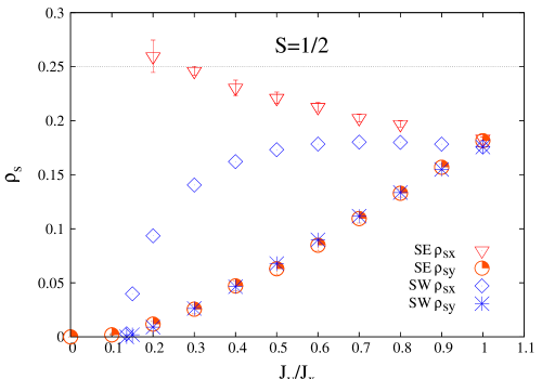
Figure 1: (Color online) Series Expansion (SE) and Spin-Wave (SW) spin-stiffness of the spin-half Heisenberg model on the anisotropic square lattice along the x and y axis as a function of the anisotropy $J_{y}/J_{x}$. The dotted line shows the value of the spin-stiffness $\rho_{sx}$ in the 1D limit of the model ($J_{y}/J_{x}=0$).

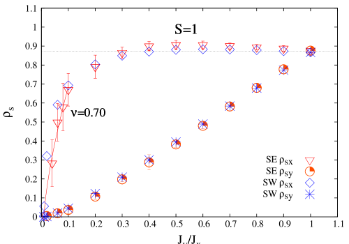
Figure 2: (Color online) Series Expansion (SE) and Spin-Wave (SW) spin-stiffness of the spin-one Heisenberg model on the anisotropic square lattice along the x and y axis as a function of the anisotropy $J_{y}/J_{x}$. In the region $0.01\leq J_{y}\leq 0.1$ the data points for the SE $\rho_{sx}$ have been fitted to the curve $\rho_{sx}=(J_{y}-0.01)^{\nu}$, with $\nu=0.7\pm 0.1$. The dotted line represents the spin-stiffness in the 2D isotropic limit of the model ($J_{y}/J_{x}=1$).

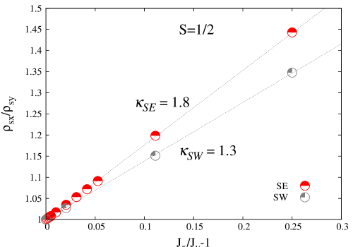
Figure 3: (Color online) Series Expansion (SE) and Spin-Wave (SW) spin-stiffness anisotropy $\rho_{sx}/\rho_{sy}$ as a function of $J_{x}/J_{y}-1$ for the spin-half Heisenberg model on the anisotropic square lattice. The data points have been fitted to the linear function given in Eq. (5) yielding $\kappa_{SE}=1.8$ and $\kappa_{SW}=1.3$

Table 1: Series expansion coefficients for the spin-stiffness of the spin-1/2 Heisenberg model on the anisotropic square lattice for selected values of the anisotropy coupling $J_{y}$.

order	$J_{x}$	$J_{y}$	$\rho_{sx}$	$\rho_{sy}$
0	1	0.9	0.2500000000	0.2250000000
1			0.0892857142	0.0698275862
2			-0.0927175942	-0.0926628428
3			-0.0151861349	-0.0132149279
4			-0.0045297105	-0.0011224771
5			0.0003357042	0.0021422839
6			-0.0057755038	-0.0049661531
7			-0.0003145877	-0.0002219010
8			-0.0042654841	-0.0038964097
0	1	0.7	0.2500000000	0.1750000000
1			0.1041666666	0.0453703703
2			-0.0868950718	-0.0850367899
3			-0.0172969207	-0.0105492432
4			-0.0045937341	0.0050836143
5			-0.0012261711	0.0039781766
6			-0.0059912113	-0.0040000116
7			-0.0006353314	-0.0005917251
8			-0.0045520522	-0.0033419898
0	1	0.5	0.2500000000	0.1250000000
1			0.1250000000	0.0250000000
2			-0.0891666666	-0.0779166666
3			-0.0235044642	-0.0081537698
4			0.0013212991	0.0140706091
5			-0.0017270061	0.0056040091
6			-0.0060489454	-0.0045071391
7			-0.0009351484	-0.0017589857
8			-0.0057105087	-0.0027490512
0	1	0.3	0.2500000000	0.0750000000
1			0.1562500000	0.0097826086
2			-0.1094346417	-0.0666305597
3			-0.0408511573	-0.0052660964
4			0.0234241580	0.0242642206
5			0.0016805213	0.0056385893
6			-0.0085614425	-0.0079166392
7			-0.0010470671	-0.0031407541
8			-0.0085663482	-0.0003268242

Table 2: Series expansion coefficients for the spin-stiffness of the spin-1 Heisenberg model on the anisotropic square lattice for selected values of the anisotropy coupling $J_{y}$.

order	$J_{x}$	$J_{y}$	$\rho_{sx}$	$\rho_{sy}$
0	1	0.9	1.0000000000	0.9000000000
1			0.1515151515	0.1208955223
2			-0.1535289080	-0.1422381534
3			0.0207519434	0.0193249175
4			-0.0428180052	-0.0391942098
5			0.0072984862	0.0068989716
6			-0.0210286555	-0.0190202422
7			0.0043677522	0.0041430202
0	1	0.7	1.0000000000	0.7000000000
1			0.1724137931	0.0803278688
2			-0.1553008729	-0.1192091787
3			0.0196401862	0.0152963896
4			-0.0421528844	-0.0313929868
5			0.0066352559	0.0055840695
6			-0.0210149617	-0.0149157761
7			0.0040511283	0.0034008244
0	1	0.5	1.0000000000	0.5000000000
1			0.2000000000	0.0454545454
2			-0.1688941361	-0.0982465564
3			0.0182177620	0.0106543293
4			-0.0421971280	-0.0242928541
5			0.0050652115	0.0041087839
6			-0.0210666888	-0.0106538747
7			0.0035338724	0.0025923026
0	1	0.3	1.0000000000	0.3000000000
1			0.2380952380	0.0183673469
2			-0.2069165600	-0.0746342335
3			0.0173382982	0.0055030901
4			-0.0479905685	-0.0189077310
5			0.0002743242	0.0023851969
6			-0.0213911544	-0.0061871738
7			0.0021597090	0.0016832884

We consider Antiferromagnetic Heisenberg model on a square-lattice, with spatially anisotropic exchange couplings given by the Hamiltonian

$$\mathcal{H}=J_{x}\sum_{\vec{r}}{\vec{S}_{\vec{r}}\cdot{\vec{S}_{\vec{r}+\hat{x}}+J_{y}\sum_{\vec{r}}{\vec{S}_{\vec{r}}\cdot{\vec{S}_{\vec{r}+\hat{y}}}}}}\ ,$$ (1)

where the sum over $\vec{r}$ runs over all sites of the square-lattice. Spin-stiffness can be defined by the change in the ground state energy of the system under an applied twist along one of the axesSingh and Huse (1989); Hamer et al. (1994). In general, it can be decomposed into a sum of two parts, a paramagnetic part and a diamagnetic part. For the anisotropic model, one can define two different twists $\rho_{sx}$ and $\rho_{sy}$ depending on whether the twist is applied along the $x$ or the $y$ axis. Following Ref. Singh and Huse, 1989; Hamer et al., 1994, the diamagnetic component of the twist for $\rho_{sy}$ is given by the expression

$$\rho_{sy}^{dia}=-J_{y}<S_{\vec{r}}^{z}S_{\vec{r}+\hat{y}}^{z}+S_{\vec{r}}^{x}S_{\vec{r}+\hat{y}}^{x}>\ ,$$ (2)

where angular brackets denote expectation value in the ground state of the Hamiltonian in Eq. (1). The paramagnetic term is given by the equation

$$\rho_{sy}^{para}=2E_{\theta}\ ,$$ (3)

where $E_{\theta}$ is the coefficient of the $\theta^{2}$ term in the ground state energy per site of the Hamiltonian in Eq. (1) with a perturbation

$$\mathcal{H}^{para}=J_{y}\theta\sum_{\vec{r}}S^{x}_{\vec{r}}(S^{z}_{\vec{r}+\hat{y}}-S^{z}_{\vec{r}-\hat{y}})\ .$$ (4)

In order to calculate these quantities we introduce an Ising anisotropyOitmaa et al. (2006) by scaling all XY parts of the exchange interactions by a factor $\lambda$. Then $\rho_{sx}$ and $\rho_{sy}$ can be calculated as a power series in $\lambda$ for any value of the coupling anisotropy. Series expansions for selected values of the anisotropy for the spin-half and spin-one model are given in Table 1 and Table 2 respectively.

The series are analyzed by Integrated Differential Approximants (IDA)Oitmaa et al. (2006). Before the analysis, a change of variable of the form $\sqrt{1-\lambda}=(1-y)$ has been introduced to remove leading singularities as $\lambda\to 1$. The results for the spin-half model are shown in Fig. 1 and the results for spin-one model are shown in Fig. 2. In the 1D limit, the spin-stiffness constant is know to be $0.25J$ from exact calculations by Shastry and SutherlandShastry and Sutherland (1990). This value is clearly larger than the square-lattice case where $\rho_{s}\approx 0.18J$. Our results are more accurate away from the 1D limit, but they clearly appear to approach the 1D limit in a smooth and monotonic manner. For the spin-one case it is known that the Neél order disappears at an anisotropy ratio of approximately $J_{y}/J_{x}=0.01$Affleck (1989); Pardini and Singh . The transition should be in the universality class of the 3D Heisenberg model. The spin-stiffness should vanish at the transition with an exponent of $\nu=0.7$Sachdev (1995). The fit shows that the data agrees well with these expectations.

For the spin-half case we also fit the small anisotropy regime to a linear behavior. The results are shown in Fig. 3 where they are compared to the spin-wave results discussed in the next section. We find that the anisotropy can be expressed as

$$\rho_{sx}/\rho_{sy}=1+\kappa(J_{x}/J_{y}-1)\ ,$$ (5)

where $\kappa=1.8$. This deviates significantly from the naive expectation $\kappa=1$.

II Spin-wave calculation

In this Section we consider the self-consistent version of spin-wave theoryIrkhin et al. (1999); Katanin and Irkhin (2007); Takahashi (1989). To apply this approach we subdivide the lattice into sublattices $A$ and $B$ and use the Dyson-Maleev representation for spin operators on each sublattice,

$$S_{i}^{+} = \sqrt{2S}a_{i}\,,\;S_{i}^{z}=S-a_{i}^{\dagger}a_{i},\;i\in A$$ (6)

$$S_{i}^{-} = \sqrt{2S}(a_{i}^{\dagger}-\frac{1}{2S}a_{i}^{\dagger}a_{i}^{\dagger}a_{i})$$

and

$$S_{i}^{+} = \sqrt{2S}b_{i}^{\dagger}\,,\;S_{i}^{z}=-S+b_{i}^{\dagger}b_{i},\;i\in B$$ (7)

$$S_{i}^{-} = \sqrt{2S}(b_{i}-\frac{1}{2S}b_{i}^{\dagger}b_{i}b_{i}),$$

where $a_{i}^{\dagger},a_{i},$ and $b_{i}^{\dagger},b_{i}$ are the Bose operators. Introducing the operators

$$B_{i}=\left\{\begin{array}[]{cc}a_{i}&i\in A\\ b_{i}^{\dagger}&i\in B\end{array}\right.$$ (8)

and decoupling the four-boson terms in the Hamiltonian into all possible two-boson combinations, we derive (see Refs. Irkhin et al., 1999; Katanin and Irkhin, 2007)

$$\mathcal{H}_{\text{SSWT}}=\sum_{i,\delta}J_{\delta}\gamma_{\delta}\left(B_{i}^{\dagger}B_{i}-B_{i+\delta}^{\dagger}B_{i}\right)\ ,$$ (9)

where $\delta=x,y$ correspond to the nearest neighbour sites in the x and y directions,

$$\gamma_{\delta}=\overline{S}+\langle a_{i}b_{i+\delta}\rangle$$ (10)

are the short-range order parameters and

$$\overline{S}=\langle S_{i\in A}^{z}\rangle=-\langle S_{i\in B}^{z}\rangle$$

is the sublattice magnetization. Diagonalizing the Hamiltonian (9) one finds the self-consistent equations at $T=0$

$$\gamma_{\delta} = \overline{S}+\sum_{\mathbf{k}}\frac{\Gamma_{\mathbf{k}}}{2E_{\mathbf{k}}}\cos k_{\delta}$$

$$\overline{S} = S+1/2-\sum_{\mathbf{k}}\frac{\Gamma_{0}}{2E_{\mathbf{k}}}\ ,$$ (11)

where the antiferromagnetic spin-wave spectrum has the form

$$E_{\mathbf{k}}=\sqrt{\Gamma_{\mathbf{0}}^{2}-\Gamma_{\mathbf{k}}^{2}}\ ,$$ (12)

with

$$\Gamma_{\mathbf{k}}=2\left(J_{x}\gamma_{x}\cos k_{x}+J_{y}\gamma_{y}\cos k_{y}\right)$$ (13)

and $\Gamma_{\mathbf{0}}\equiv\Gamma_{\mathbf{k}=0}$ (we assume here that the ground state is antiferromagnetically ordered, otherwise a bosonic chemical potential $\mu\neq 0$ should be introduced in the dispersion (12) to fulfill the condition $\overline{S}=0$, see Refs. Irkhin et al., 1999; Katanin and Irkhin, 2007). The parameters $\gamma_{\delta}$ are simply related to the spin correlation function at the nearest-neighbor sites by

$$\gamma_{\delta}=|\langle\mathbf{S}_{i}\mathbf{S}_{i+\delta}\rangle|^{1/2}.$$ (14)

The spin-wave stiffnes along the x and y axes is expressed through these parameters as

$$\rho_{s\delta}=J_{\delta}S\overline{S}\gamma_{\delta}$$ (15)

The results obtained according to Eqs. (11) and (15) are shown in Figs. 1, 2. While for $S=1$ the spin-wave results are close to those obtained by series expansions over the entire parameter range, for $S=1/2$ at large anisotropy, the two techniques give results for $\rho_{sy}$ which are qualitatively different. This difference is most probably due to topological excitations within the half-integer spin chains, which are not considered by spin-wave theory. For $S=1$, at the transition to the Haldane phase, we find the stiffness exponents to be $\nu_{x}=0.50$ and $\nu_{y}=1.07$, in qualitative agreement with series expansions.

For $S=1/2$, a quantitative discrepancy between spin-wave theory and series expansions is visible already at small anisotropies. While series expansion and spin-wave stiffness along the weaker exchange couplings axis ($J_{y}$) remain very close to each other, a discrepancy arises from the stiffness along the stronger coupling direction. We find the coefficient in the linear fit (5) $\kappa_{\text{SW}}=1.3,$ somewhat lower than what found by series expansion, as shown in Fig 3. It is possible that part of the difference is due to numerical inaccuracies or high order effects in $1/S$. However, with increasing anisotropy the difference is not just quantitative. It becomes qualitative and it implies the onset of new physics for the spin-half case associated with the Berry phase terms Sachdev (1995).

III Pinning

We base our considerations on the theory of underdoped cuprates suggested in Ref. Milstein and Sushkov, . According to this theory, the ground state of an underdoped uniformly doped cuprate is a spin spiral, spontaneously directed along the (1,0) or the (0,1) direction. At sufficiently small doping, $x<x_{c}$, the spiral has a static component while at $x>x_{c}$ it is fully dynamic. Here $x$ is the concentration of holes in CuO₂ plane. According to this picture, the electronic liquid crystal observed in Ref. Hinkov2007, ; Hinkov et al., 2008 is the mostly dynamic spin spiral which may still have some small static component. For Sr doped La₂CuO₄, the value of the critical concentration is $x_{c}\approx 0.11$, and for YBa₂Cu₃O_6.+y is $x_{c}\approx 0.09$. The absolute value of the wave vector of the spin spiral (static or dynamic) is given by

$$Q=\frac{g}{\rho_{s}}x\ .$$ (16)

Here $\rho_{s}\approx 0.18J$ is the spin-stiffness of the initial Heisenberg model Singh and Huse (1989), $J\approx 130meV$ is the antiferromagnetic exchange parameter of the model, and $g$ is the coupling constant for the interaction between mobile holes and spin waves. We set the spacing of the tetragonal lattice equal to unity, so the the wave vector $Q$ is dimensionless. To fit the neutron scattering experimental data to the position of the incommensurate structure in Sr doped single layer La₂CuO₄, we need to set $g\approx J$, and to fit similar data for double layer YBa₂Cu₃O_6.+y, we need to set $g\approx 0.7J$. It is not clear yet why the values of $g$ for these compounds are slightly different, but for purposes of the present work this difference is not important. The coupling constant $g$ was calculated within the extended t-J model Igarashi and Fulde (1992); Sushkov and Kotov (2004). The result is $g=Zt$ where $t$ is the nearest site hopping matrix element and $Z$ is the quasihole residue. It is known that in cuprates $t\approx 3J$ and $Z\approx 0.3$. Thus the calculated value of the coupling constant, $g\approx J$, agrees well with that found by fitting of experimental data. The ground state energy of the spin spiral state consists of two parts. The spin spiral with the wave vector $Q$ gives rise to the gain $-gQ$ in the kinetic energy of a single hole. On the other hand the spiral costs the spin elastic energy $\rho_{s}Q^{2}/2$. So the total balance is $E=\rho_{s}Q^{2}/2-xgQ$, and minimization with respect to $Q$ gives the wave vector (16) and the energy per elementary cell

$$E=\rho_{s}Q^{2}/2-xgQ=-\frac{Z^{2}t^{2}x^{2}}{2\rho_{s}}\ .$$ (17)

There are also quantum corrections to this energy, but they are small and hence not important for our purposesMilstein and Sushkov . Note, that Eq. (17) is valid for both $x<x_{c}$ and $x>x_{c}$, assuming that $x$ is not large.

Up to now we have disregarded the anisotropy assuming a perfect square lattice. To analyze anisotropy in the spiral direction we have to replace

$$t\to t(1\pm\epsilon)\ ,$$ (18)

where $\epsilon$ is due to the lattice deformation, so $t_{a}=t(1+\epsilon)$ and $t_{b}=t(1-\epsilon)$. The antiferromagnetic exchange, $J\propto t^{2}/U$, also becomes anisotropic, $J_{a}=J(1+2\epsilon)$, $J_{b}=J(1-2\epsilon)$. Hence the spin-stiffness is replaced by $\rho_{s}\to\rho_{s}(1\pm 2\kappa\epsilon)$, where $\kappa\approx 1.8$ has been calculated above. Now we can see how the lattice deformation influences the spiral energy (17). In the case when ${\bm{Q}}$ is directed along the $a^{*}=(1,0)$ we have to replace in (17) $t\to t_{a}$ and $\rho_{s}\to\rho_{sa}$; and in the case when ${\bm{Q}}$ is directed along the $b^{*}=(0,1)$ we have to replace in (17) $t\to t_{b}$ and $\rho_{s}\to\rho_{sb}$. Note that the quasiparticle residue $Z$ is a scalar property and therefore it is independent of direction of ${\bm{Q}}$. Altogether, with account of the anisotropy, the energy (17) is replaced by

$$E\to-\frac{g^{2}x^{2}}{2\rho_{s}}\left[1\mp 2(\kappa-1)\epsilon\right]\ .$$ (19)

The minus sign corresponds to $\mathbf{Q}$ directed along the $a^{*}=(1,0)$ axis, and the plus sign corresponds to $\mathbf{Q}$ directed alone the $b^{*}=(0,1)$ axis. Interestingly, without the spin-quantum-fluctuations effect (i. e. if $\kappa=1$) the anisotropy in energy disappears.

Since $a^{*}<b^{*}$ it is most natural to assume that $t_{a}>t_{b}$, This means that $\epsilon>0$. This point is supported by the LDA calculation performed in Ref. Andersen et al., 1995. In this case, according to Eq. (19), the energy of the state with $\mathbf{Q}$ along the $a^{*}$-axis is higher than that with $\mathbf{Q}$ along the $b^{*}$-axis. This disagrees with the experimental data in Ref. Hinkov2007, ; Hinkov et al., 2008. However, the anisotropy of the hopping matrix element $t$ is not straightforward. There are two competing contributions to $\epsilon$. The first one is related to the lattice deformation and is positive. The second one is related to oxygen chains that are present in YBa₂Cu₃O_6.45 and is negative. In principle it is possible for the negative contribution to win, making $\epsilon$ negative PC . The neutron scattering anisotropy has been previously discussed within the Pomeranchuk instability scenario Yamase and Metzner (2006). This is probably not sufficient to explain the newest data, see discussion in Ref. Yamase, . However, it is interesting to note that, to explain the sign of the pinning, the Pomeranchuk scenario also requires a negative $\epsilon$. Anyway, for further numerical estimates, we will assume

$$\epsilon\approx-0.02$$ (20)

The absolute value is consistent with the 1% lattice deformation and the sign has been discussed above. In this case, according to Eq. (19), the energy of the state with $\mathbf{Q}$ along the $a^{*}$-axis is lower and this is consistent with experimental data. The direction of pinning energy at $x=0.09$ reads

$$\epsilon(\kappa-1)\frac{g^{2}x^{2}}{\rho_{s}}\sim 5\times 10^{-2}meV$$ (21)

This is the pinning energy per Cu site and it is a pretty strong pinning. For comparison, the pinning energy of spin to the orthorhombic b-direction in undoped La₂CuO₄ is just $\sim 1.5\times 10^{-3}meV$. Assuming that the correlation length is at least comparable with the period of the spin spiral, $\xi\sim 2\pi/Q\sim 17$, we find that the total pinning energy per correlation unit is $\sim 5\times 10^{-2}\xi^{2}\sim 15meV$, which is a significant energy scale.

IV conclusions

In this paper, we have studied the spin-stiffness constants for spatially anisotropic spin-half and spin-one Heisenberg models using series expansions and self-consistent spin-wave theory. The theoretical results have been of interest in themselves and show the importance of Berry phase interference terms in anisotropic square-lattice models.

Our primary motivation for the study has been to understand the phenomena of electronic liquid crystal and its pinning in high temperature superconductors. We find that quantum interference effects significantly enhance the spin-stiffness anisotropy and this can provide the primary mechanism for the pinning of the liquid crystal direction. We have provided a detailed quantitative account of the pinning energy in YBCO.

- (1) V. Hinkov, P. Bourges, S. Pailhes, Y. Sidis, A. Ivanov, C. D. Frost, T. G. Perring, C. T. Lin, D. P. Chen, B. Keimer, Nature Physics 3, 780 (2007).
- Hinkov et al. (2008) V. Hinkov, D. Haug, B. Fauque, P. Bourges, Y. Sidis, A. Ivanov, C. Bernhard, C. T. Lin, and B. Keimer, Science 319, 597 (2008).
- Affleck and Halperin (1996) I. Affleck and B. I. Halperin, Journal of Physics A: Mathematical and General 29, 2627 (1996).
- Affeck et al. (1994) I. Affeck, M. P. Gelfand, and R. R. P. Singh, Journal of Physics A: Mathematical and General 27, 7313 (1994).
- Parola et al. (1993) A. Parola, S. Sorella, and Q. F. Zhong, Phys. Rev. Lett. 71, 4393 (1993).
- Sandvik (1999) A. W. Sandvik, Phys. Rev. Lett. 83, 3069 (1999).
- Irkhin and Katanin (2000) V. Y. Irkhin and A. A. Katanin, Phys. Rev. B 61, 6757 (2000).
- Shastry and Sutherland (1990) B. S. Shastry and B. Sutherland, Phys. Rev. Lett. 65, 243 (1990).
- Sachdev (1995) S. Sachdev, Low Dimensional Quantum Field Theories for Condensed Matter Physicists (World Scientific, Singapore, 1995), edited by Y. Lu, S. Lundqvist, and G. Morandi.
- Singh and Huse (1989) R. R. P. Singh and D. A. Huse, Phys. Rev. B 40, 7247 (1989).
- Hamer et al. (1994) C. J. Hamer, Z. Weihong, and J. Oitmaa, Phys. Rev. B 50, 6877 (1994).
- Oitmaa et al. (2006) J. Oitmaa, C. Hamer, and W. Zheng, Series Expansion Methods for Strongly Interacting Lattice Models (Cambridge University Press, New York, 2006).
- Affleck (1989) I. Affleck, Phys. Rev. Lett. 62, 474 (1989).
- (14) T. Pardini and R. R. P. Singh, arXiv:0801.3855v1 [cond-mat.str-el].
- Irkhin et al. (1999) V. Y. Irkhin, A. A. Katanin, and M. I. Katsnelson, Phys. Rev. B 60, 1082 (1999).
- Katanin and Irkhin (2007) A. A. Katanin and V. Y. Irkhin, Physics-Uspekhii 50, 613 (2007).
- Takahashi (1989) M. Takahashi, Phys. Rev. B 40, 2494 (1989).
- (18) A. I. Milstein and O. P. Sushkov, arXiv:0711.4865.
- Igarashi and Fulde (1992) J.-i. Igarashi and P. Fulde, Phys. Rev. B 45, 10419 (1992).
- Sushkov and Kotov (2004) O. P. Sushkov and V. N. Kotov, Phys. Rev. B 70, 024503 (2004).
- Andersen et al. (1995) O. K. Andersen, A. I. Lichtenstein, O. Jepsen, and F. Paulsen, J. Phys. Chem. Solids 56, 1573 (1995).
- (22) O. K. Andersen, private communication.
- Yamase and Metzner (2006) H. Yamase and W. Metzner, Physical Review B 73, 214517 (2006).
- (24) H. Yamase, arXiv:0802.1149 [cond-mat.str-el].