Quantum Computation in a radio-single mode cavity: the dissipative Jaynes and Cummings Model

Abstract

In this paper we have considered the interaction of a Jaynes and Cummings system with the electromagnetic field in its vacuum state and, solving the dynamical problem, we have analyzed the amount of entanglement induced in the bipartite system (atom + cavity mode) by the common electromagnetic reservoir. This has allowed us to quantitatively characterize the regime under which field-induced cooperative effects are not vanished by dissipation. Once the Decoherence Free Regime is reached, transient entanglement tends to become stationary and, therefore, usable for quantum gate implementation.

1 Introduction

The idea of implementing quantum information devices based on the use of single atoms or molecules has gone progressively growing up in the course of the last few years. The reason can be envied in the high contemporary evolution of theoretical dynamical models along with the ability reached by experimentalists in manipulating quantum objects first considered theoretician’s tools raimond . The state of art is that, although it has been possible to obtain entanglement conditions between elementary systems in different physical scenarios raimond , the temporal persistence of quantum coherence is an open problem. In this moment, it is therefore necessary to put attention on the theoretical aspects of decoherence in order to predict the experimental conditions under which it is maximally reduced palma . Almost Decoherence Free Substates seem to have the characteristics of eligibility needed to implement quantum computation. Their generation and temporal persistence can be theoretically predicted in some high symmetrical models nud ; Nicolosi ; NicolosiPRL ; tesi ; Plenio1999 ; Pellizzari ; Ficek03 . The application of the formal solution of the Markovian Master Equation (Nud theorem) nud has supplied, in the few analyzed systems, the prediction of a conditional building up of entanglement. The result is obtained under symmetrical condition corresponding to specific locations of involved subsystems (atoms, molecules). Unfortunately, despite the positive results in isolating single quantum objects raimond , the difficulties connected with the location of more than one atoms in fixed arbitrary points is an open task.

Contrarily, the isolation of a single atom for enough long time inside a cavity is today possible. A single mode cavity and a two level atom may be considered a hybrid two qubits system. Moreover, the Jaynes and Cummings Model describing this system is one of the few exactly soluble models in quantum optics. It predicts many interesting non classical states experimentally testable in laboratory raimond . In realistic situation, however, one performs experiments in cavity with finite Q and in presence of atomic spontaneous emission. So it become of fundamental importance to know how the predictions of this model are affected by the unavoidable presence of loss mechanisms. This problem is currently very extensively studied, the main approximation being the assumption of two different reservoirs, one for the atom and one for the cavity mode respectively raimond2 . The Lindblad master equation describing this model is easy to solve, the solution being the total destruction of coherences because of the two different and nonspeaking channels of dissipation. Contrarily to this approach, we assume a common bath of interaction between the cavity mode and the atom. The master equation so derived contains the simple one as particular case. In this paper we show to be able to find the exact solution of a dissipative J-C model assuming a common reservoir for the bipartite system, which, on the ground of the above consideration, appears to be a more realistic hypothesis. This leads to the prediction of new cooperative effects, induced by the zero-point fluctuations of environment, between the atom and the cavity mode as the creation of conditional transient entanglement, tending to become stationary as the strengths of the coupling with the reservoir take a well defined value. Finally, in order to be maximally realistic, we consider also the loose of energy due to the imperfect reflection on the mirrors. This correction in the microscopic model does not introduce complication in the solution of the relative master equation because the new bath is independent from the first one and, indeed, easily treating from a theoretical point of view (not induced coherences). In presence of the second channel of decoherence the building up of entanglement exists during the transient period in which the atom is confined inside the cavity. The long time solution (the order of magnitude of the time involved is given in the next sections) shows that the introduction of the second bath makes disappear coherence (Rabi oscillation) among the two subsystem involved: the atom and the cavity mode. Despite this fact, the time involved in decoherence process can be made much longer than those necessary to implement a quantum protocol as deducible from the theoretical analysis here developed if interfaced with the experimental measures performed by Haroches’ group. The measure of the probability to find the atom in the excited state appear well fitted by the theoretical model here proposed. The standard models (two different baths) are able to reproduce only the top of the curve of atomic population. Instead our is able to reproduce also the lower part.

The paper is structured as follow: in section II we report the principal step and approximation leading to the microscopic derivation of the Markovian Master Equation and we solve it when $T=0$, showing also the full equivalence between MME and Piecewise Deterministic Processes (PDP) nud . In section III we apply the NuD theorem to derive the solution to the dissipative J-C model. In section IV we report the main conclusion of the paper.

2 The Markovian Master Equation

It is well know that under the Rotating Wave and the Born-Markov approximations the master equation describing the reduced dynamical behavior of a generic quantum system linearly coupled to an environment can be put in the form nud ; F.Petruccione

$$\dot{\rho_{S}}(t)=-i[H_{S}+H_{LS},\rho_{S}(t)]+D(\rho_{S}(t)),$$ (1)

where $H_{S}$ is the Hamiltonian describing the free evolution of the isolated system,

$$D(\rho_{S}(t)) = \sum_{\omega}\sum_{\alpha,\beta}\gamma_{\alpha,\beta}(\omega)(A_{\beta}(\omega)\rho_{S}(t)A^{{\dagger}}_{\alpha}(\omega)$$ (2)

$$- \frac{1}{2}\{A^{{\dagger}}_{\alpha}(\omega)A_{\beta}(\omega),\rho_{S}(t)\}),$$

$$H_{LS}=\sum_{\omega}\sum_{\alpha,\beta}S_{\alpha,\beta}(\omega)A^{\dagger}_{\alpha}(\omega)A_{\beta}(\omega),$$ (3)

$$S_{\alpha,\beta}(\omega)=\frac{1}{2i}(\Gamma_{\alpha,\beta}(\omega)-\Gamma^{\ast}_{\beta,\alpha}(\omega))$$ (4)

and

$$\gamma_{\alpha,\beta}(\omega)=\Gamma_{\alpha,\beta}(\omega)+\Gamma^{\ast}_{\beta,\alpha}(\omega),$$ (5)

$\Gamma_{\alpha,\beta}(\omega)$ being the one-sided Fourier transforms of the reservoir correlation functions. Finally we recall that the operators $A_{\alpha}(\omega)$ and $A_{\alpha}^{{\dagger}}(\omega)$, we are going to define and whose properties we are going to explore, act only in the Hilbert space of the system.

Eq. (1) has been derived under the hypothesis that the interaction Hamiltonian between the system and the reservoir, in the Schrödinger picture, is given by F.Petruccione

$$H_{I}=\sum_{\alpha}A^{\alpha}\otimes B^{\alpha},$$ (6)

that is the most general form of the interaction.

In the above expression $A^{\alpha}=(A^{\alpha})^{\dagger}$ and $B^{\alpha}=(B^{\alpha})^{\dagger}$ are operators acting respectively on the Hilbert space of the system and of the reservoir. The eq. (6) can be written in a slightly different form if one decomposes the interaction Hamiltonian into eigenoperators of the system and reservoir free Hamiltonian.

Definition 1

Definition Supposing the spectrum of $H_{S}$ and $H_{B}$ to be discrete (generalization to the continuous case is trivial) let us denote the eigenvalue of $H_{S}$ ($H_{B}$) by $\varepsilon$ ($\eta$) and the projection operator onto the eigenspace belonging to the eigenvalue $\varepsilon$ ($\eta$) by $\Pi(\varepsilon)$ ($\Pi(\eta)$). Then we can define the operators:

$$A_{\alpha}(\omega)\equiv\sum_{\varepsilon^{{}^{\prime}}-\varepsilon=\omega}\Pi(\varepsilon)A_{\alpha}\Pi(\varepsilon^{{}^{\prime}}),$$ (7)

$$B_{\alpha}(\omega)\equiv\sum_{\eta^{{}^{\prime}}-\eta=\omega}\Pi(\eta)B_{\alpha}\Pi(\eta^{{}^{\prime}}).$$ (8)

From the above definition we immediately deduce the following relations

$$[H_{S},A_{\alpha}(\omega)]=-\omega A_{\alpha}(\omega),$$ (9)

$$[H_{B},B_{\alpha}(\omega)]=-\omega B_{\alpha}(\omega),$$

$$[H_{S},A^{{\dagger}}_{\alpha}(\omega)] = +\omega A^{{\dagger}}_{\alpha}(\omega)\;\;\;and$$ (10)

$$[H_{B},B^{{\dagger}}_{\alpha}(\omega)] = +\omega B^{{\dagger}}_{\alpha}(\omega).$$

An immediate consequence is that the operators $A^{{\dagger}}_{\alpha}(\omega>0)$ e $A_{\alpha}(\omega>0)$ raise and lower the energy of the system $S$ by the amount $\hbar\omega$ respectively and that the corresponding interaction picture operators take the form

$$e^{iH_{S}t}A_{\alpha}(\omega)e^{-iH_{S}t}=e^{-i\omega t}A_{\alpha}(\omega),$$ (11)

$$e^{iH_{B}t}B_{\alpha}(\omega)e^{-iH_{B}t}=e^{-i\omega t}B_{\alpha}(\omega),$$

$$e^{iH_{S}t}A^{{\dagger}}_{\alpha}(\omega)e^{-iH_{S}t}=e^{+i\omega t}A^{{\dagger}}_{\alpha}(\omega)\;\;\;and$$ (12)

$$e^{iH_{B}t}B^{{\dagger}}_{\alpha}(\omega)B^{-iH_{B}t}=e^{+i\omega t}B^{{\dagger}}_{\alpha}(\omega).$$

Finally we note that

$$A^{{\dagger}}_{\alpha}(\omega)=A_{\alpha}(-\omega)\;\;\;and\;\;\;B^{{\dagger}}_{\alpha}(\omega)=B_{\alpha}(-\omega).$$ (13)

Summing eq. (13) over all energy differences and employing the completeness relation we get

$$\sum_{\omega}A^{{\dagger}}_{\alpha}(\omega)=\sum_{\omega}A_{\alpha}(-\omega)=A_{\alpha}\;\;\;and$$ (14)

$$\sum_{\omega}B^{{\dagger}}_{\alpha}(\omega)=\sum_{\omega}B_{\alpha}(-\omega)=B_{\alpha}$$

The above positions enable us to cast the interaction Hamiltonian into the following form

$$H_{I}=\sum_{\alpha,\omega,\omega^{\prime}}A_{\alpha}(\omega)\otimes B_{\alpha}(\omega^{\prime})=$$ (15)

$$\sum_{\alpha,\omega,\omega^{\prime}}A^{{\dagger}}_{\alpha}(\omega)\otimes B^{{\dagger}}_{\alpha}(\omega^{\prime}).$$

The reason for introducing the eigenoperator decomposition, by virtue of which the interaction Hamiltonian in the interaction picture can now be written as

$$H_{I}(t)=\sum_{\alpha,\omega,\omega^{\prime}}e^{-i(\omega+\omega^{\prime})t}A_{\alpha}(\omega)\otimes B_{\alpha}(\omega^{\prime}),$$ (16)

is that exploiting the rotating wave approximation, whose microscopic effect is to drop the terms for which $\omega\neq-\omega^{\prime}$, is equivalent to the Schrodinger picture interaction Hamiltonian:

$$H_{I}=\sum_{\alpha,\omega}A_{\alpha}(\omega)\otimes B_{\alpha}(-\omega)=\sum_{\alpha,\omega}A_{\alpha}(\omega)\otimes B^{{\dagger}}_{\alpha}(\omega).$$ (17)

Theorem 2.1

Lemma The Rotating Wave Approximation imply the conservation of the free energy of the global system, that is

$$[H_{S}+H_{B},H]=0$$ (18)

2.1 Proof

The necessary condition involved in the previous proposition is equivalent to the equation $[H_{S}+H_{B},H_{I}]=0$ we are going to demonstrate.

$$[H_{S}+H_{B},H] = [H_{S}+H_{B},H_{I}]$$

$$= [H_{S},H_{I}]+[H_{B},H_{I}]$$

$$= \sum_{\alpha,\omega}[H_{S},A_{\alpha}(\omega)]\otimes B_{\alpha}^{{\dagger}}(\omega)+$$

$$\sum_{\alpha,\omega}A_{\alpha}(\omega)\otimes[H_{B},B_{\alpha}^{{\dagger}}(\omega)]$$

$$= -\sum_{\alpha,\omega}\omega A_{\alpha}(\omega)\otimes B_{\alpha}(-\omega)+$$

$$\sum_{\alpha,\omega}\omega A_{\alpha}(\omega)\otimes B_{\alpha}(-\omega)=0.$$

where we have made use of eq. (9,10)  

Theorem 2.2

Lemma The detailed balance condition in the thermodynamic limit imply Alicki

$$\gamma_{\alpha\beta}(\omega)=e^{-\beta\omega}\gamma_{\alpha\beta}(-\omega)$$ (20)

where $\beta=(k_{B}T)^{-1}$  

Theorem 2.3

Corollary Let us suppose the temperature of the thermal reservoir to be the absolute zero, on the ground of Lemma 2 immediately we see that

$$\gamma_{\alpha\beta}(\omega<0)=0\;\;\;\rule{5.0pt}{5.0pt}$$ (21)

Let us now cast eq. (1) in a slightly different form splitting the sum over the frequency, appearing in eq. (2), in a sum over the positive frequencies and a sum over the negative ones so to obtain

$$D(\rho_{S}(t))$$ (22)

$$= \sum_{\omega>0,\alpha,\beta}\gamma^{\alpha,\beta}(\omega)(A^{\beta}(\omega)\rho_{S}A^{\alpha{\dagger}}(\omega)$$

$$- \frac{1}{2}\{A^{\beta{\dagger}}(\omega)A^{\alpha}(\omega),\rho_{S}\})$$

$$+ \sum_{\omega>0,\alpha,\beta}\gamma^{\alpha,\beta}(-\omega)(A^{\alpha{\dagger}}(\omega)\rho_{S}A^{\beta}(\omega)$$

$$- \frac{1}{2}\{A^{\alpha}(\omega)A^{\beta{\dagger}}(\omega),\rho_{S}\}),$$

where we again make use of eq. (13). In the above expression we can recognize the first term as responsible of spontaneous and stimulated emission processes, while the second one takes into account stimulated absorption, as imposed by the lowering and raising properties of $A^{\alpha}(\omega)$. Therefore if the reservoir is a thermal bath at $T=0$ the corollary 4 tell us that the correct dissipator of the Master Equation can be obtained by suppressing the stimulated absorption processes in eq. (22).

2.2 NuD Theorem

We are now able to solve the markovian master equation when the reservoir is in a thermal equilibrium state characterized by $T=0$. We will solve a Cauchy problem assuming the factorized initial condition to be an eigenoperator of the free energy $H_{S}+H_{B}$. This hypothesis doesn’t condition the generality of the found solution being able to extend itself to an arbitrary initial condition because of the linearity of the markovian master equation .

Theorem 2.4

NuD theorem If eq. (1) is the markovian master equation describing the dynamical evolution of a open quantum system S, coupled to an environment B, assumed to be in the detailed-balance thermal equilibrium state characterized by a temperature T=0, and if the global system is initially prepared in a state $\rho(0)=\rho_{B}(0)\rho_{S}(0)$ so that $(H_{S}+H_{B})\rho(0)(H_{S}+H_{B})=E_{L}^{2}\rho(0)$, where $E_{L}=E_{S}+E_{B}$ is the free energy of the global system then $\rho_{S}(t)$ is in the form of a Piecewise Deterministic Process F.Petruccione , that is a process obtained combining a deterministic time-evolution with a jump process.

The proof of the theorem is contained in the paper nud . My aim here is to give an explanation of the found implication.

A PDP is a statistical mixture of alternative generalized trajectories evolving individually in a deterministic way. This statement is mathematically given by the equation

$$\rho_{S}(t)=\sum_{i=0}^{N}\rho_{i}(t),$$ (23)

where the quantum trajectories $\rho_{i}(t)$ are obtained by the deterministic non-unitary equation

$$\rho_{i}(t)=U(t)f_{i}(t)U^{{\dagger}}(t),$$ (24)

where, in particular,

$$f_{N}(t)=\rho_{N}(0)$$ (25)

and $U(t)=e^{-\frac{i}{\hbar}Bt}$, $U^{\dagger}(t)=e^{\frac{i}{\hbar}B^{\dagger}t}$, $B$ being

$$B=H_{0}-\frac{i}{2\hbar}\sum_{\omega>0,\alpha,\beta}\gamma^{\alpha\beta}(\omega)A^{\beta{\dagger}}(\omega)A^{\alpha}(\omega)\equiv H_{0}-\frac{i}{2\hbar}H^{\prime},$$ (26)

with $H^{\prime}$ hermitian. Finally,

$$f_{N-j} (t)=\sum_{\omega^{\prime},\alpha^{\prime},\beta^{\prime}}\sum_{\omega",\alpha",\beta"}$$

$$... \sum_{\omega^{j},\alpha^{j},\beta^{j}}\gamma^{\alpha\beta}(\omega)\gamma^{\alpha^{\prime}\beta^{\prime}}(\omega^{\prime})\gamma^{\alpha"\beta"}(\omega")...\gamma^{\alpha^{j}\beta^{j}}(\omega^{j})$$

$$\times \int_{0}^{t}\int_{0}^{t^{\prime}}\int_{0}^{t"}...\int_{0}^{t^{j}}dt^{\prime}dt"...dt^{j}$$

. $$U^{-1}(t^{\prime})A^{\beta^{\prime}}(\omega^{\prime})U(t^{\prime})U^{-1}(t")A^{\beta"}(\omega")U(t")$$

$$... U^{-1}(t^{j})A^{\beta^{j}}(\omega^{j})U(t^{j})f_{N}(t^{j})U^{{\dagger}}(t^{j})A^{\alpha^{j}{\dagger}}(\omega^{j})U^{{\dagger}-1}(t")$$

$$... U^{{\dagger}}(t")A^{\alpha"{\dagger}}(\omega")U^{{\dagger}-1}(t")U^{{\dagger}}(t^{\prime})A^{\alpha^{\prime}{\dagger}}(\omega^{\prime})U^{{\dagger}-1}(t^{\prime}),$$

$$j =1,...,N\;\;\;\rule{5.0pt}{5.0pt}$$

These last are generalized respect to F.Petruccione and H.J.Carmochael approach, which leads to $\rho_{S}(t)=\sum_{i}|\psi_{i}><\psi_{i}|$. The last expansion, in terms of proper trajectories, is obtainable from ours if and only if we are able to put into diagonal form the spectral correlation tensor, that is known to be always possible because of the positivity of $\gamma^{\alpha\beta}$, but nobody is able to do it, with exception of few highly symmetrical systems.

The found solution (NuD theorem) ensures that the dynamical processes, whose statistical mixture gives the open system stochastic evolution, are deterministic. This demonstrates that the evolution is representable as a Piecewise Deterministic Process (PDP) F.Petruccione . The found solution generalizes the PDPs introduced by H.J.Carmichael and formalized by F.Petruccione and H.P.Breuer. Actually, it is applicable also when the Markovian Master Equation isn’t in the Lindblad form. This, as already highlighted, in general, introduces simplification in the further calculations, but because of the difficulty to recast the equation in this form the results obtained are in general merely formal. Tough the eq. (2.2) seems complicated to use it is a powerful predictive tool. We have tested it deriving the photocounting formula tesi ; Davies ; reproducing the environment-induced entanglement between two two-level not-direct-interacting atoms placed in fixed arbitrary points in the free space tesi ; Plenio1999 ; Pellizzari ; Ficek03 and Carmichael unravelling of the Master Equation tesi ; Carmichael .

Moreover, we have tested the NuD theorem’s predictive capability solving the dynamics of two two-level dipole-dipole interacting atoms placed in fixed arbitrary points inside a single mode cavity in presence of atomic spontaneous emission and cavity losses NicolosiPRL ; $n$ two-level not-direct-interacting atoms placed in fixed arbitrary points inside a single mode cavity in presence of atomic spontaneous emission and cavity losses Nicolosi ; a bipartite hybrid model, known as Jaynes-Cummings model, constituted by an atom and a single mode cavity linearly coupled and spontaneously emitting in the same environment (next subsection) and two harmonic oscillator linearly coupled and spontaneously emitting in the same environment (work in progress).

3 Dissipative Jaynes and Cummings model

The Jaynes-Cummings Model describes, under the Rotating Wave Approximation, the resonant interaction between a single two-level atom and the single mode of the electromagnetic field protected by a perfect cavity (no loosing of energy). The model has been introduced in 1963 Jaynes in order to analyze the classical aspects of spontaneous emission and to understand the effects of quantization on the atomic evolution. Actually, despite its apparent simplicity, this model has revealed interesting non-classical proprieties characterizing the matter-radiation interaction. Moreover, thanks to the recent experimental implementation of high Q cavities, it is today possible to verify the most of the theoretical predictions of the model raimond ; raimond2 ; raimond3 .

The major experimental limitation is related to the coupling with a chaotic environment able to destroy the quantum coherences. A theoretical approach including the loss of energy due to the interaction of the atom and the cavity mode with the free electromagnetic field is more complete and, as we will show, it is suitable to reproduce the experimental measured decay of the population of the atom raimond . In particular, assuming a common bath of interaction between the cavity mode and the atom, the theoretical probability to find the atom in the excited state performs Rabi oscillation exponentially decaying. This fact is consistent with the open dynamics but it is not the only effect. Actually, the common bath induces cooperation between the two involved parts (mode and atom). This behavior competes with the exponential decay. In the long time limit the the exponential decay wins on cooperation if we work under the experimental condition performed by Haroche group. In the paper raimond is reported the experimental graph relative to the probability to find the atom in its excited state as a function of the time. We can interpret the upper part of the figure as the exponential decay and the lower part of it (increasing of probability) as the cooperation induced by the common reservoir. The new theoretical approach, here presented, is better than the usual one (two independent baths) because it is able to reproduce the experimental curve in a complete way. In fact the two bath approximation keeps account only for the dissipation meaning that the Rabi oscillation of the atomic population goes to zero every period characterizing the free dynamics of the bipartite system. In this case the cooperative part of the dynamics disappears: the two parts do not speak trough the common bath, the main behavior being the dissipation of energy in the reservoirs. Moreover it is possible to demonstrate that single bath approach is more general than the other including it as particular case. This fact is very well understood if the parts are, for example, two or more atoms, in which case the cooperation is the maximum one if the distance among atoms is small enough and it reaches its minimum value when the distance goes to infinity Nicolosi . In the last case the out diagonal terms of the spectral correlation tensor go to zero meaning that the parts see independent reservoirs. The lack of a microscopical derivation of the coupling constant of the mode with the electromagnetic field makes difficult the analytical derivation of an analogue relation in the case here analyzed. Despite this fact it will be shown that the single bath case is more general than the other one because the independent baths case does not reproduce the out diagonal terms giving a simplified Master Equation unable to reproduce part of the experimental measurements.

The Hamiltonian describing the open system is

$$H = \hbar\frac{\omega_{0}}{2}S_{z}+\hbar\omega_{0}\alpha^{\dagger}\alpha+\hbar(\epsilon\alpha S_{+}+\epsilon^{\ast}\alpha^{\dagger}S_{-})$$

$$+ \hbar\sum_{\vec{k},\lambda}\omega_{\vec{k}}b^{\dagger}_{\lambda}(\vec{k})b_{\lambda}(\vec{k})$$

$$+ \sum_{\vec{k},\lambda}[g^{\ast}_{\vec{k},\lambda}b_{\lambda}(\vec{k})+g_{\vec{k},\lambda}b^{{\dagger}}_{\lambda}(\vec{k})](S_{+}+S_{-})$$

$$+ \sum_{\vec{k},\lambda}[s^{\ast}_{\vec{k},\lambda}b_{\lambda}(\vec{k})+s_{\vec{k},\lambda}b^{{\dagger}}_{\lambda}(\vec{k})](\alpha^{\dagger}+\alpha).$$

If we make the position

$$H_{S}=\hbar\frac{\omega_{0}}{2}S_{z}+\hbar\omega_{0}\alpha^{\dagger}\alpha+\hbar(\epsilon\alpha S_{+}+\epsilon^{\ast}\alpha^{\dagger}S_{-}),$$ (29)

$$H_{B}=\hbar\sum_{\vec{k},\lambda}\omega_{\vec{k}}b^{\dagger}_{\lambda}(\vec{k})b_{\lambda}(\vec{k}),$$ (30)

$$H_{I}=\sum_{\alpha=1}^{2}A^{\alpha}B^{\alpha},$$ (31)

where

$$B^{1}=\sum_{\vec{k},\lambda}[g^{\ast}_{\vec{k},\lambda}b_{\lambda}(\vec{k})+g_{\vec{k},\lambda}b{{}^{\dagger}}_{\lambda}(\vec{k})],$$ (32)

$$B^{2}=\sum_{\vec{k},\lambda}[s^{\ast}_{\vec{k},\lambda}b_{\lambda}(\vec{k})+s_{\vec{k},\lambda}b{{}^{\dagger}}_{\lambda}(\vec{k})]$$ (33)

$$A^{1}=(S_{+}+S_{-}),$$ (34)

$$A^{2}=(\alpha^{\dagger}+\alpha)$$ (35)

we can describe the reduced dynamics of the bipartite system at $T=0$ by a Master Equation of the standard form

$$\dot{\rho_{S}}(t)=-\frac{i}{\hbar}[H_{S},\rho_{S}(t)]+D(\rho_{S}(t)).$$ (36)

In this expression we have neglected the Lamb-Shift. This approximation is made possible because we have considered, ab initio, a direct linear static interaction among the parts respect to which the Lamb-Shift is negligible. In the above equation

$$D(\rho_{S}(t)) = \gamma^{1,1}(S_{-}\rho_{S}S_{+}-\frac{1}{2}\{S_{+}S_{-},\rho_{S}\})$$

$$+ \gamma^{2,2}(\alpha\rho_{S}\alpha^{\dagger}-\frac{1}{2}\{\alpha^{\dagger}\alpha,\rho_{S}\})$$

$$+ \gamma^{1,2}(\alpha\rho_{S}S_{+}-\frac{1}{2}\{\alpha^{\dagger}S_{-},\rho_{S}\})$$

$$+ \gamma^{2,1}(S_{-}\rho_{S}\alpha^{\dagger}-\frac{1}{2}\{S_{+}\alpha,\rho_{S}\})$$

where

$$\gamma^{1,1}=\pi\sum_{\vec{k},\lambda}\mid g_{\vec{k}\lambda}\mid^{2}\delta(\omega_{\vec{k}}-\omega)$$ (38)

$$\gamma^{2,2}=\pi\sum_{\vec{k},\lambda}\mid s_{\vec{k}\lambda}\mid^{2}\delta(\omega_{\vec{k}}-\omega)$$ (39)

$$\gamma^{1,2} = \pi\sum_{\vec{k},\lambda}Re(s^{\ast}_{\vec{k}\lambda}g_{\vec{k}\lambda})\delta(\omega_{\vec{k}}-\omega)$$

$$+ i\hbar\pi\sum_{\vec{k},\lambda}Im(s^{\ast}_{\vec{k}\lambda}g_{\vec{k}\lambda})\delta(\omega_{\vec{k}}-\omega)$$

$$\gamma^{2,1} = \pi\sum_{\vec{k},\lambda}Re(s^{\ast}_{\vec{k}\lambda}g_{\vec{k}\lambda})\delta(\omega_{\vec{k}}-\omega)$$

$$- i\hbar\pi\sum_{\vec{k},\lambda}Im(s^{\ast}_{\vec{k}\lambda}g_{\vec{k}\lambda})\delta(\omega_{\vec{k}}-\omega)$$

The master equation for $\rho_{S}$ can be solved applying the NuD theorem to this case:

$$\rho_{S}(t)=\sum_{i=0}^{n}\rho_{i}(t),\;\;\;\;i\in N$$ (42)

where $n$ is the number of the excitation initially given to the system ($\rho_{S}(0)\equiv\rho_{n}(0)$) and $i$ is the index giving the number of excitations characterizing every quantum trajectory.

The trajectories evolve in time in accordance with

$$\rho_{i}(t)=N(t)f_{i}(t)N^{{\dagger}}(t),$$ (43)

where $f_{i}(t)$ is given by eq.(2.2) and $N(t)=e^{-\frac{i}{\hbar}}Bt$ is a nonunitary temporal evolution operator, $B$ being, in general, non-hermitian as it appears from the following equation:

$$B=\frac{\hbar}{2}\Omega_{0}S_{z}+\hbar\Omega\alpha^{\dagger}\alpha+MS_{+}\alpha+P\alpha^{\dagger}S_{-}-i\frac{\gamma^{1,1}}{2},$$ (44)

where

$$\Omega_{0}=\omega_{0}-i\gamma^{1,1}$$ (45)

$$\Omega=\omega_{0}-i\gamma^{2,2}$$ (46)

$$M=\varepsilon-i\gamma^{2,1}$$ (47)

$$P=\varepsilon^{\ast}-i(\gamma^{2,1})^{\ast}.$$ (48)

Let us suppose the system in the initial state characterized by $(n-1)$ excitations in the cavity mode and the atom in its excited state $\mid+>$:

$$\rho_{S}(0)=\mid(n-1),+><(n-1),+\mid,$$ (49)

then every quantum trajectory $\rho_{i}(t)$ belonging to statistical mixture characterizing the dynamical evolution of the system will have the form

$$\rho_{i}(t) = \rho_{1,1_{i}}(t)\mid(i-1),+><(i-1),+\mid$$

$$+ \rho_{1,2_{i}}(t)\mid(i-1),+><i,-\mid$$

$$+ \rho_{2,1_{i}}(t)\mid i,-><(i-1),+\mid$$

$$+ \rho_{2,2_{i}}(t)\mid i,-><i,-\mid.$$

The highest energy subspace ($i=n$) is easily solved and the block vector relative to this subspace has the form:

$$\rho_{1,1_{n}}(t) = \frac{e^{-2\gamma_{2,2}\left(n-\frac{1}{2}\right)t-\gamma_{1,1}t}}{2\mid A_{n}\mid^{2}}\{(\mid A_{n}\mid^{2}-\mid\Delta\mid^{2})$$

. $$\cos(2a_{n}t)+(\mid A_{n}\mid^{2}+\mid\Delta\mid^{2})\cosh(2b_{n}t)$$

$$- 2ib_{n}\Delta(\sin(2a_{n}t)+\sinh(2b_{n}t))\}$$

$$\rho_{1,2_{n}}(t) = \frac{i\sqrt{n}M^{\ast}}{2A_{n}^{\ast}}e^{-2\gamma_{2,2}\left(n-\frac{1}{2}\right)t-\gamma_{1,1}t}$$

. $$\{\sin(2a_{n}t)-i\sinh(2b_{n}t)$$

$$+ i\frac{\Delta}{A_{n}}(\cos(2a_{n}t)-\cosh(2b_{n}t))\}$$

$$\rho_{2,1_{n}}(t)=\rho^{\ast}_{1,2_{n}}(t)$$ (53)

$$\rho_{2,2_{n}}(t) = \frac{n\mid M\mid^{2}}{4\mid A_{n}\mid^{2}}e^{-2\gamma_{2,2}\left(n-\frac{1}{2}\right)t-\gamma_{1,1}t}$$

. $$\{\sin(2a_{n}t)-i\sinh(2b_{n}t)\},$$

where

$$A_{n} = a_{n}+ib_{n}=\sqrt{\Delta^{2}+nMP}$$ (55)

$$\Delta = \frac{1}{2}(\gamma_{1,1}-\gamma_{2,2}).$$ (56)

Let us note that if we have started from the initial condition $\mid\psi_{1}(0)>=\mid n,->$ we have obtained the same dynamical behavior. This fact ensures that an arbitrary linear combination of the two different initial condition will bring to the same dynamics. This fact is really important because it is not simple to prepare one or the other of the initial states. Actually, when we inject an excitation inside the system we can only know that the system is in a statistical mixture of the two states. But we have seen seen that the dynamics is not case sensitive and therefore a statistical mixture of the two states leads to the described dynamical evolution.

3.1 Entanglement building up

The circumstance that we succeed in finding the explicit time dependence of the solution of the master equation (36) provides an occasion to analyze in detail at least some aspects of how entanglement is getting established in our bipartite system. As particular case we can choose $n=1$ so obtaining in a simple way the complete dynamics of the open system in the form

$$\rho_{S}(t)=\rho_{0}(t)+\rho_{1}(t),$$ (57)

where

$$\rho_{1}(t) = \rho_{1,1_{1}}(t)\mid 0,+><0,+\mid$$

$$+ \rho_{1,2_{1}}(t)\mid 0,+><1,-\mid$$

$$+ \rho_{2,1_{1}}(t)\mid 1,-><0,+\mid$$

$$+ \rho_{2,2_{1}}(t)\mid 1,-><1,-\mid$$

and

$$\rho_{0}(t)=(1-\rho_{1,1_{1}}(t)-\rho_{2,2_{1}}(t))\mid 0,-><0,-\mid$$ (59)

On the basis of the block diagonal form exhibited by Eq. (57), at a generic time instant $t$, the system is in a statistical mixture of the vacuum state of the system and of a one-excitation appropriate density matrix describing with certainty the storage of the initial energy. In order to analyze the time evolution of the degree of entanglement that gets established between the two initially uncorrelated parties, we exploit the concept of concurrence $C$ first introduced by Wootters Wootters97 ; Wootters98 . If, at an assigned time $t$, no photon have been emitted the conditional concurrence $C$ assumes the form:

$$C(t) = \sqrt{\frac{2(\rho_{1,1_{n}}\rho_{2,2_{n}}+\mid\rho_{1,2_{n}}\mid^{2})+4\rho_{2,2_{n}}\mid\rho_{1,2_{n}}}{\rho_{1,1_{n}}+\rho_{2,2_{n}}}}$$

$$- \sqrt{\frac{2(\rho_{1,1_{n}}\rho_{2,2_{n}}+\mid\rho_{1,2_{n}}\mid^{2})-4\rho_{2,2_{n}}\mid\rho_{1,2_{n}}}{\rho_{1,1_{n}}+\rho_{2,2_{n}}}}.$$

In the analyzed case ($n=1$), as clearly shown in Fig.1, obtained using the experimental values setted by Haroche’s group, the degree of entanglement (C(t)) starting from zero increases during the transient collapsing to the initial value when time is long enough. This fact depend on the choice of the atom whose spontaneous emission time $\gamma_{1,1}$ is much longer than the cavity damping time $\gamma_{2,2}$. In accordance to this fact the probability to find the atom in the excited state starting from $1$ go to zero when $t\gg(\gamma_{1,1}+\gamma_{2,2})^{-1}$ as clearly showed in Fig.2. This Figure reproduce in a perfect way the experimental measures performed by Haroche’s group raimond . The standard theoretical models assume two different channel of dissipation (one for the atom and one for the cavity mode). The corresponding Master Equation is simpler to solve because of the absence of cooperative terms nud but the corresponding dynamics fits only the upper part of the measures of the Haroche’s group (dissipative behavior). The low part of the graph represent the cooperation induced by the common reservoir between the cavity mode and the atom.

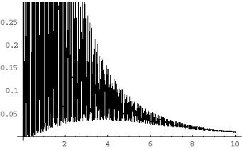
Figure 1: $\gamma_{1,1}=1/30KHz$, $\gamma_{2,2}=1KHz$, $\gamma_{1,2}=\gamma_{2,1}=1/\sqrt{30}KHz$ , $\epsilon=47\pi KHz$ , t=10=1ms

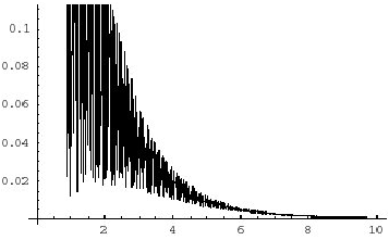
Figure 2: $\gamma_{1,1}=1/30KHz$, $\gamma_{2,2}=1KHz$, $\gamma_{1,2}=\gamma_{2,1}=1/\sqrt{30}KHz$ , $\epsilon=47\pi KHz$ , t=10=1ms

Such cooperation become the maximum one when $\gamma_{1,1}=\gamma_{2,2}$, as clearly shown in Fig.3 and Fig.4. These ones depicted the concurrence and the probability to find the atom in its excited state, respectively.

Under this condition (Decoherence Free Regime) Eq. (57) suggests that, for $t\gg(\gamma_{1,1}+\gamma_{2,2})^{-1}$, the correspondent asymptotic form assumed by $\rho_{S}(t)$ is time independent and such that the probability of finding energy in the bipartite system is $\frac{1}{2}$:

$$\rho_{S}(t\gg(\gamma_{1,1}+\gamma_{2,2})^{-1})=\frac{1}{2}\mid\psi_{G}><\psi_{G}\mid$$ (61)

$$+\frac{1}{2}\mid\psi_{A}><\psi_{A}\mid,$$

where

$$\mid\psi_{G}>=\mid 0,-><0,-\mid$$ (62)

is the ground state of the bipartite system and

$$\mid\psi_{A}>=\frac{1}{\sqrt{2}}(\mid 0,+><1,-\mid-\mid 1,-><0,+\mid)$$ (63)

is the maximally antisymmetric entangled state of the system.

This fact suggests that stationary entangled states of the JC system can be generated by putting a single photon detector able to capture in a continuous way all the excitations lost by the system in the reservoir. Reading out the detector states at $t\gg(\gamma_{1,1}+\gamma_{2,2})^{-1}$, if no photons have been emitted, then, as a consequence of the measurement outcome, our system is projected into the maximally antisymmetric entangled state $\mid\psi>=\frac{1}{\sqrt{2}}(\mid 0,+><1,-\mid-\mid 1,-><0,+\mid)$.

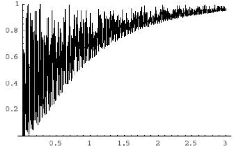
Figure 3: $\gamma_{1,1}=1KHz$, $\gamma_{2,2}=1KHz$, $\gamma_{1,2}=\gamma_{2,1}=1KHz$ , $\epsilon=47\pi KHz$ , t=10=1ms

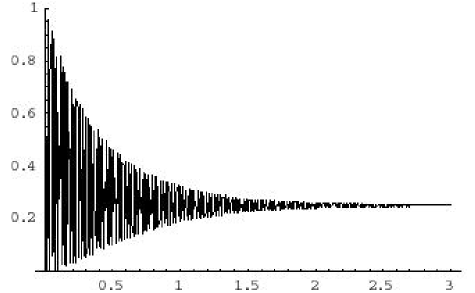
Figure 4: $\gamma_{1,1}=1KHz$, $\gamma_{2,2}=1KHz$, $\gamma_{1,2}=\gamma_{2,1}=1KHz$ , $\epsilon=47\pi KHz$ , t=10=1ms

This is the main result of the paper which means that a successful measurement, performed at large enough time instants, generates un uncorrelated state of the two subsystems, bipartite system and reservoir, leaving atom and cavity in their maximally antisymmetric entangled state.

This ideal result has to be corrected by the introduction in the microscopical model of a second bath of interaction able to take account of the cavity leakage of energy because of the imperfect mirrors. In terms of the hamiltonian operator this means:

$$H = \hbar\frac{\omega_{0}}{2}S_{z}+\hbar\omega_{0}\alpha^{\dagger}\alpha+\hbar(\epsilon\alpha S_{+}+\epsilon^{\ast}\alpha^{\dagger}S_{-})$$

$$+ \hbar\sum_{\vec{k},\lambda}\omega_{\vec{k}}b^{\dagger}_{\lambda}(\vec{k})b_{\lambda}(\vec{k})+\hbar\sum_{\vec{k},\lambda}\omega_{\vec{k}}c^{\dagger}_{\lambda}(\vec{k})c_{\lambda}(\vec{k})$$

$$+ \sum_{\vec{k},\lambda}[g^{\ast}_{\vec{k},\lambda}b_{\lambda}(\vec{k})+g_{\vec{k},\lambda}b^{{\dagger}}_{\lambda}(\vec{k})](S_{+}+S_{-})$$

$$+ \sum_{\vec{k},\lambda}[s^{\ast}_{\vec{k},\lambda}b_{\lambda}(\vec{k})+s_{\vec{k},\lambda}b^{{\dagger}}_{\lambda}(\vec{k})](\alpha^{\dagger}+\alpha)$$

$$+ \sum_{\vec{k},\lambda}[r^{\ast}_{\vec{k},\lambda}c_{\lambda}(\vec{k})+r_{\vec{k},\lambda}c^{{\dagger}}_{\lambda}(\vec{k})](\alpha^{\dagger}+\alpha).$$

If we make the position

$$H_{S}=\hbar\frac{\omega_{0}}{2}S_{z}+\hbar\omega_{0}\alpha^{\dagger}\alpha+\hbar(\epsilon\alpha S_{+}+\epsilon^{\ast}\alpha^{\dagger}S_{-}),$$ (65)

$$H_{B}=\hbar\sum_{\vec{k},\lambda}\omega_{\vec{k}}b^{\dagger}_{\lambda}(\vec{k})b_{\lambda}(\vec{k})+\hbar\sum_{\vec{k},\lambda}\omega_{\vec{k}}c^{\dagger}_{\lambda}(\vec{k})c_{\lambda}(\vec{k}),$$ (66)

$$H_{I}=\sum_{\alpha=1}^{2}A^{\alpha}B^{\alpha},$$ (67)

where

$$B^{1}=\sum_{\vec{k},\lambda}[g^{\ast}_{\vec{k},\lambda}b_{\lambda}(\vec{k})+g_{\vec{k},\lambda}b{{}^{\dagger}}_{\lambda}(\vec{k})],$$ (68)

$$B^{2} = \sum_{\vec{k},\lambda}[s^{\ast}_{\vec{k},\lambda}b_{\lambda}(\vec{k})+s_{\vec{k},\lambda}b{{}^{\dagger}}_{\lambda}(\vec{k})]$$

$$+ \sum_{\vec{k},\lambda}[r^{\ast}_{\vec{k},\lambda}c_{\lambda}(\vec{k})+r_{\vec{k},\lambda}c{{}^{\dagger}}_{\lambda}(\vec{k})]$$

$$A^{1}=(S_{+}+S_{-}),$$ (70)

$$A^{2}=(\alpha^{\dagger}+\alpha)$$ (71)

we can describe the reduced dynamics of the bipartite system at $T=0$ by a standard Master Equation and we can solve it in the same way of the previous case. The changes in the microscopical model do not introduce variation in the formal solution. Instead, the presence of two different channel of dissipation modifies the dynamical behavior. Actually, the system has now the possibility to loose energy in environments that do not speak each other. This means that, when the time is much longer than the sum of the single emission time, the coherence induced by the common bath during the transient will go to zero in the long time domain. Despite this fact, the dechoerence time can be made as long as we need to implement the required quantum protocol. Actually, named $k$ the cavity decay rate, if $k$ is much greater than $\gamma_{1,1}=\gamma_{2,2}$, then the storage of energy can be maximized for a time sufficient to realize the quantum protocol.

4 Conclusion

In this paper we have considered the interaction of a Jaynes and Cummings system with the electromagnetic field (and with another phenomenological zero temperature bath) in its vacuum state and, solving the dynamical problem, we have analyzed the amount of entanglement induced in the bipartite system by the common electromagnetic reservoir. This has allowed us to quantitatively characterize the regime under which field-induced cooperative effects are not vanished by dissipation. Once the Decoherence Free Regime is reached, transient entanglement tends to become stationary and, therefore, usable for quantum gate implementation.

The asymptotic solution of the dynamical problem appears to be a statistical mixture of a maximally entangled state and the ground state of the open system, the probability to obtain one or the others being the same. In the whole temporal domain the found solution tell us that the state of the system is a statistical mixture of the free energy system eigenoperators. This fact is general enough nud and it is consistent with the existence of a photon detector device because the act of measurement introduces a stochastic variable respect to which we can only predict the probability to have one or another of the possible alternative measures nud . These probabilities can be regarded as the weight of the possible alternative generalized trajectories. With this approach the dynamics has to be depicted as a statistical mixture of this alternative generalized trajectories. Moreover the found trajectories evolve in time in a deterministic way: for example the trajectory relative to the initially excited system state is a shifted free evolution characterized by complex frequencies that means an exponential decay free evolution. This statement may give the sensation that every system has to decay in its ground state because of the observed dynamics. It is in general not true. Actually, if the system is multipartite as ours, it is possible that it admits excited and entangled equilibrium Decoherence Free Subspace (DFS) Lidar (so as it happens in some highly symmetric models), constituted by states on which the action of $H_{I}$ is identically zero. If the system, during evolution, passes through one of these states, the successive dynamics will be decoupled from the environment evolution. An equilibrium condition is reached in which entanglement is embedded in the system.

References

- (1) J.M.Raimond, M.Brune, S.Haroche, Rev. Mod. Phys., 73, 565 (2001)
- (2) T. Nirrengarten, A. Qarry, C. Roux, A. Emmert, G. Nogues, M. Brune, J.-M. Raimond, and S. Haroche, Phys. Rev. Lett., 97, 200405 (2006)
- (3) G.M. Palma, K-A Suominen, A. Ekert, Quantum computers and dissipation, Proc. Roy. Soc. Lond. A 452 567-584 (1996)
- (4) S.Nicolosi, Open Systems and Information Dynamics 12, (2005)
- (5) E. Knill, R. Laflamme, H. Barnum, D. Dalvit, J. Dziarmaga, J. Gubernatis, L. Gurvits, G. Ortiz, L. Viola, W.H. Zurek quant-ph/0207171
- (6) S. Nicolosi, A. Napoli, A. Messina, Eurp Phys Jour D 1 115 (2005)
- (7) S. Nicolosi, A. Napoli, A. Messina , F.Petruccione Phys Rev A 70 022511 (2004)
- (8) S.Nicolosi, Soluzione operatoriale esatta di master equation ottiche generalizzate: applicazioni a problemi di interazione radiazione materia, Thesis (2003), unpublished
- (9) Plenio, Huelga, Beige, Knight, Phys. Rev. A 59 (1999) 2468
- (10) T. Pellizzari, S.A. Gardiner, J.I. Cirac, P.Zoller, Phys. Rev. Lett. 75, 3788 (1995)
- (11) Z.Ficek, R.Tanas, quant-ph 0302124
- (12) A.Olaya-Castro, Niel F.Johnson, quant-ph0306104 (2004), to appear in Handbook of Theoretical and Computational Nanotecnology
- (13) F.Petruccione, H.P.Breuer, The Theory of open quantum sistem, Oxford University Press (2002)
- (14) C.W.Gardiner, Quantum Noise, Springer-Verlag Berlin (1991)
- (15) W.H.Louiselle, Quantum statistical properties of radiation, Ed. John Wiley e Sons (1973)
- (16) R.Alicki, K.Lendi, Quantum Dynamical Semigroups and Applications, Lectures Notes in Physics V286, (Springer-Verlag 1987)
- (17) H.Carmichael, An Open System Approach to Quantum Optics, Lectures Notes in Physics m18, (Springer-Verlag 1993)
- (18) Y.Castin, K.Molmer, Phys. Rev. Lett. 74, 3772 (1995)
- (19) J.Dalibard, Y.Castin, K.Molmer, Phys. Rev. Lett. 68, 580 (1992)
- (20) E.B.Davies, Commun. Math. Phys. 15, 277 (1969)
- (21) M.D.Srinivas, E.B.Davies, Opt. Acta 28, 981 (1981)
- (22) M.B.Plenio, P.L.Knight, Rev. Mod. Phys. 70, 101 (1998)
- (23) F.Petruccione, H.P.Breuer, Concepts and methods in the theory of open quantum systems systems, Lectures Notes in Physics V622, Springer-Verlag Berlin (2003)
- (24) H.J. Carmichael and K. Kim, Optics Commun. 179, 417 (2000)
- (25) J.P. Clemens, L. Horvath, B.C. Sanders, and H.J. Carmichael, Phys. Rev. A 68, 023809 (2003)
- (26) V.B.Braginsky, F.Ya.Khalili, Quantum Measurement, Cambridge University Press (1992)
- (27) S.M.Barnett, P.M.Radmore, Methods in Theoretical Quantum Optics, Oxford Series in Optical and Imaging Science, 15 (2002)
- (28) C.Leonardi, F.Persico, G.Vetri, La rivista del Nuovo Cimento9(1986) 3,4
- (29) G.Benivegna A.messina, J.Mod.Opt. 36 (1989) 1205
- (30) M.Kozierowski, S.M.Chumakov, A.A.Mamedov, Journal of Mod. Opt. 40 (1993)453
- (31) B.W.Shore, P.L.Knight, Journal of Mod. Opt. 40 (1993)7
- (32) I.K.Kudryavstev, A.Lambrecht, H.Moya-Cessa, P.L.Knight, Journal of Mod. Opt. 40 (1993)8
- (33) S.J.D.Phoenix, S.M.Barnett, Journal of Mod. Opt. 40 (1993)6
- (34) Dicke, phys. rep. 93 (1954)99
- (35) M. A. Nielsen and I. L. Chuang, Quantum Computation and Quantum Information, Cambridge University Press, Cambridge, (2000).
- (36) Guo Ping Guo et al, Phys. Rev. A 65, 042102 (2002)
- (37) Lu-Ming Duan et al, Phys. Rev. A 58, (1998)
- (38) J.I.Cirac, P.Zoller, Phys. Rev. A 50, R2799 (1993)
- (39) Shneider, Milburn, Phys. Rev. A 65, 042107 (2002)
- (40) G.J.Yang, O.Zobay, P.Meystre, Phys. Rev. A 59, 4012 (1998)
- (41) E.Hagley, X.Maitre, G.Nogues, C.Wunderlich, M.Brune, J.M.Raimond, S.Haroche, Phys. Rev. Lett. 79, 1 (1997)
- (42) P.Foldi, M.G.Benedict, A.Czirjak, Phys. Rev. A 65, 021802 (2002)
- (43) M. Brune, F. Schmidt-Kaler, A. Maali, J. Dreyer, E. Hagley, J. M. Raimond, S. Haroche Phys. Rev. Lett. 76, 1800 (1996)
- (44) S. Hill, W. K. Wootters Phys. Rev. Lett. 78, 5022-5025 (1997)
- (45) W. K. Wootters Phys. Rev. Lett. 80, 2245-2248 (1998)
- (46) D.A.Lidar, B.Whaley quant-ph/0301032