Large deviation function for entropy production in driven one-dimensional systems

Abstract

The large deviation function for entropy production is calculated for a particle driven along a periodic potential by solving a time-independent eigenvalue problem. In an intermediate force regime, the large deviation function shows pronounced deviations from a Gaussian behavior with a characteristic “kink” at zero entropy production. Such a feature can also be extracted from the analytical solution of the asymmetric random walk to which the driven particle can be mapped in a certain parameter range.

The mathematical theory of large deviations is concerned with the exponential decay of the probability of extreme events while the number of observations grows Ellis (2006). In driven systems coupled to a heat reservoir, energy in the form of heat is dissipated and therefore entropy in the surrounding medium is produced. The large deviation function of the entropy production rate in nonequilibrium steady states is a frequently studied quantity (see Ref. Harris and Schütz (2007) and references therein) for basically two reason. First, since entropy is produced on average, the large deviation function captures the asymptotically time-independent behavior of the probability distribution for the entropy production. Second, the large deviation function exhibits a special symmetry called fluctuation theorem or Gallavotti-Cohen symmetry. First seen in computer simulations of a sheared liquid Evans et al. (1993), the fluctuation theorem has been proven for both deterministic thermostated dynamics Gallavotti and Cohen (1995); Evans and Searles (2002) and stochastic dynamics Kurchan (1998); Lebowitz and Spohn (1999).

Analytical solutions for the large deviation function exist only for a few simple models Lebowitz and Spohn (1999); Visco (2006); van Wijland (2006). Obtaining the large deviation function over the full range from experimental data is a difficult task since trajectories leading to negative entropy production are strongly suppressed with increasing trajectory length (see, e.g., Ref. Ciliberto et al. (2004)). For a study of the complete large deviation function one therefore has to rely on computer simulations. To follow rare trajectories, different schemes have been proposed and implemented Giardinà et al. (2006); Lecomte and Tailleur (2007); Imparato and Peliti (2007). All these approaches have in common that they simulate trajectories from which the Legendre transform of the large deviation function is determined. In contrast, in this Communication we calculate numerically the Legendre transform directly as the lowest eigenvalue of an evolution operator. We therefore reduce the problem of determining a time-dependent probability distribution to solving a time-independent eigenvalue problem.

For a simple paradigmatic system, we investigate a single driven colloidal particle immersed in a fluid and trapped in a toroidal geometry by optical tweezers such that it effectively moves in one dimension Faucheux et al. (1995); Blickle et al. (2007). For short and intermediate times, the experimentally measured probability distribution for the entropy production exhibits a detailed structure with multiple peaks arising from the periodic nature of the system Speck et al. (2007). As the observation time increases, the distribution becomes more and more sharply peaked around its mean. Rare large deviations from this mean are then governed by the large deviation function, which we determine in this study. We then compare our results in a certain parameter range to the analytically solvable model of the asymmetric random walk.

The colloidal particle is driven into a nonequilibrium steady state through a constant force $f$. In addition, the particle moves within an external periodic potential $V(\varphi)$, where $0\leqslant\varphi<2\pi$ is the angular coordinate of the particle. The total force acting on the particle is $F(\varphi)=-\partial_{\varphi}V(\varphi)+f$. The overdamped motion of the particle is governed by the Langevin equation

$$\partial_{t}\varphi(t)=F(\varphi)+\zeta(t).$$ (1)

The noise $\zeta$ represents the interactions of the particle with the fluid and has zero mean and short-ranged correlations $\langle\zeta(t)\zeta(t^{\prime})\rangle=2\delta(t-t^{\prime})$. Throughout the paper, we set Boltzmann’s constant to unity, leading to a dimensionless entropy. In addition, we scale time and energy such that the bare diffusion coefficient and the thermal energy become unity.

We are interested in the large deviation function of the entropy production

$$h(\sigma)\equiv\lim_{t\rightarrow\infty}-\frac{1}{t}\ln p(s_{\mathrm{m}},t).$$ (2)

The entropy $s_{\mathrm{m}}$ produced in the heat bath during the time $t$ is a stochastic quantity with probability distribution $p(s_{\mathrm{m}},t)$. The asymptotic large fluctuations of $s_{\mathrm{m}}$ are then given by $p(s_{\mathrm{m}},t)\sim\exp[-h(\sigma)t]$, where $\sigma\equiv(s_{\mathrm{m}}/t)/\langle\dot{s}_{\mathrm{m}}\rangle$ is the dimensionless, normalized entropy production rate. We will not determine the large deviation function $h(\sigma)$ directly through evaluating $p(s_{\mathrm{m}},t)$ but from the generating function

$$g(\varphi,\lambda,t)\equiv\int_{-\infty}^{+\infty}\mathrm{d}s_{\mathrm{m}}\;e^{-\lambda s_{\mathrm{m}}}\rho(\varphi,s_{\mathrm{m}},t).$$ (3)

Here, $\rho(\varphi,s_{\mathrm{m}},t)$ is the joint probability for the particle to be at an angle $\varphi$ and to have produced an amount $s_{\mathrm{m}}$ of entropy during the time $t$. This generating function obeys the equation of motion $\partial_{t}g=\hat{L}_{\lambda}g$ with an operator $\hat{L}_{\lambda}$ yet to be determined. We can then expand $g$ into eigenfunctions $\psi_{n}(\varphi,\lambda)$ determined from the eigenvalue equation

$$\hat{L}_{\lambda}\psi_{n}(\varphi,\lambda)=-\alpha_{n}(\lambda)\psi_{n}(\varphi,\lambda).$$ (4)

The lowest eigenvalue $\alpha_{0}(\lambda)$ determines the asymptotic time dependence of the generating function $g\sim\exp[-\alpha_{0}(\lambda)t]$. In particular, the mean entropy production rate is $\langle\dot{s}_{\mathrm{m}}\rangle=\alpha_{0}^{\prime}(0)$. The large deviation function finally is the Legendre transform

$$h(\sigma)=\alpha_{0}(\lambda^{\ast})-\langle\dot{s}_{\mathrm{m}}\rangle\sigma\lambda^{\ast},\qquad\langle\dot{s}_{\mathrm{m}}\rangle\sigma=\alpha^{\prime}_{0}(\lambda^{\ast})$$ (5)

of the cumulant generating function as can be shown by a saddle-point integration. The large deviation function for the entropy production shows the symmetry relation

$$h(-\sigma)=h(\sigma)+\langle\dot{s}_{\mathrm{m}}\rangle\sigma$$ (6)

called fluctuation theorem Gallavotti and Cohen (1995); Kurchan (1998); Lebowitz and Spohn (1999). If the fluctuation theorem holds then the lowest eigenvalue exhibits an equivalent symmetry, $\alpha_{0}(\lambda)=\alpha_{0}(1-\lambda)$. Hence, it is a symmetric function centered at $\lambda=1/2$ Lebowitz and Spohn (1999).

In this approach, the asymptotic fluctuations of $s_{\mathrm{m}}$ can be extracted from the solution of the eigenvalue equation (4) for $n=0$. As an advantage compared to following definition (2), we do not have to solve a time-dependent equation of motion for $p(s_{\mathrm{m}},t)$. Instead, the information of the asymptotic fluctuations is contained in a time-independent equation which we can tackle more easily.

The entropy change along a single stochastic trajectory is defined as the functional Seifert (2005a)

$$s_{\mathrm{m}}[x(\tau)]\equiv\int_{0}^{t}\mathrm{d}\tau\;F(x(\tau))\dot{x}(\tau)=f(x-x_{0})-\Delta V.$$

The time integration implies the introduction of a second angular coordinate $x$ which takes into account the number of revolutions of the particle and measures the total traveled distance in contrast to the bounded coordinate $\varphi$. Since the terms involving $\Delta V$ and $x_{0}$ are bounded they will not contribute to the entropy production rate in the limit of large times. Hence, the expression for the entropy production in this limit simplifies to $s_{\mathrm{m}}\approx fx$.

The Fokker-Planck operator corresponding to the Langevin equation (1) reads

$$\hat{L}_{0}\equiv-\partial_{\varphi}(F-\partial_{\varphi}).$$ (7)

In the next step, we want to obtain the evolution operator $\hat{L}$ for the joint probability $\rho(\varphi,s_{\mathrm{m}},t)$ which obeys $\partial_{t}\rho=\hat{L}\rho$. This operator is then converted to the sought-after evolution operator $\hat{L}_{\lambda}$ for the generating function (3). The stochastic processes for $\varphi$ and $x$ (and hence $s_{\mathrm{m}}$) share the same noise. We can therefore replace $\partial_{\varphi}\mapsto(\partial_{\varphi}+\partial_{x})$ to obtain

$$\hat{L}=\hat{L}_{0}+(2\partial_{\varphi}-F)\partial_{x}+\partial_{x}^{2}.$$ (8)

Differentiating Eq. (3) with respect to time and inserting the operator (8) leads after partial integration to

$$\hat{L}_{\lambda}=\hat{L}_{0}+(2\partial_{\varphi}-F)f\lambda+(f\lambda)^{2}$$ (9)

with vanishing boundary terms.

For the numerical evaluation, we represent the operator $\hat{L}_{\lambda}$ as a matrix through choosing a basis. To this end, we distinguish left sided $\langle k|$ from right sided $|k\rangle$ basis states. The basis must be complete and orthonormal, $\langle k|l\rangle=\delta_{kl}$. Expanding the eigenfunctions $\psi_{n}(\lambda)=\sum_{k}c^{(n)}_{k}(\lambda)|k\rangle$ into the basis, Eq. (4) becomes

$$\sum_{l=-\infty}^{\infty}L_{kl}c^{(n)}_{l}=-\alpha_{n}(\lambda)c^{(n)}_{k},\qquad L_{kl}\equiv\langle k|\hat{L}_{\lambda}l\rangle.$$ (10)

Hence, we seek the lowest eigenvalue $\alpha_{0}(\lambda)$ of the matrix $\mathbf{L}_{\lambda}\equiv(L_{kl})$ where $\lambda$ appears as a mere parameter. A suitable choice for the basis is

$$\langle k|\varphi\rangle=\frac{e^{-\mathrm{i}k\varphi}}{\sqrt{2\pi}},\quad\langle\varphi|k\rangle=\frac{e^{+\mathrm{i}k\varphi}}{\sqrt{2\pi}},\quad\int_{0}^{2\pi}\mathrm{d}\varphi\;|\varphi\rangle\langle\varphi|=1$$ (11)

due to the periodic nature of the system.

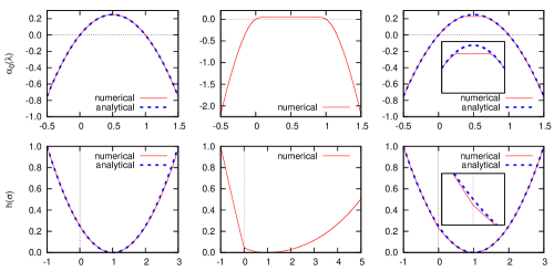
Figure 1: Eigenvalue $\alpha_{0}(\lambda)$ (top row) and large deviation function $h(\sigma)$ (bottom row) for the entropy production versus the force values $f=0.05$ (left), $f=4.05$ (center), and $f=100$ (right) for a potential depth $v_{0}=5$. The ordinates are in units of the mean production rate $\langle\dot{s}_{\mathrm{m}}\rangle$. For small and large forces, the large deviation function and therefore the eigenvalues are almost parabolic. The corresponding analytical functions (12) are shown for comparison. The insets in the right panels show the enlarged regions around $\lambda=1/2$ and $\sigma=0$, respectively.

We now specialize our analysis to a cosine potential $V(\varphi)=v_{0}\cos\varphi$ introducing a second dimensionless parameter $v_{0}$. A straightforward calculation shows that the matrix $\mathbf{L}_{\lambda}$ becomes tridiagonal with elements

$$L_{kk}=-(k-\mathrm{i}f\lambda)^{2}-\mathrm{i}f(k-\mathrm{i}f\lambda),$$

$$L_{k,k\pm 1}=\pm\frac{v_{0}}{2}(k-\mathrm{i}f\lambda).$$

We are not aware of an analytic solution for the eigenvalues of such a matrix. However, by truncating the size of the matrix to some finite value, they can easily be found numerically by standard algorithms. In Fig. 1, we show both $\alpha_{0}(\lambda)$ and the large deviation function $h(\sigma)$ of the entropy production. The fluctuation theorem (6) is fulfilled as can be seen immediately by the symmetry of $\alpha_{0}(\lambda)$. For large driving forces $f\gg v_{0}$ as depicted in the right panels, both functions are almost parabolic. In this case, the particle hardly “feels” the potential and the mean velocity becomes $\langle\dot{x}\rangle\approx f$. Integrating over the angle $\varphi$, the eigenvalue can then be read off from the operator (9) as

$$\alpha_{0}(\lambda)=\langle\dot{s}_{\mathrm{m}}\rangle\lambda(1-\lambda),\quad h(\sigma)=(\langle\dot{s}_{\mathrm{m}}\rangle/4)(\sigma-1)^{2}$$ (12)

with $\langle\dot{s}_{\mathrm{m}}\rangle\approx f^{2}$. For small forces $f\ll v_{0}$ (left panels), the particle remains mostly within one potential minimum and the mean rate becomes exponentially small in the barrier height $2v_{0}$. In this case, the large deviation function again approaches a parabola for which the symmetry (6) enforces the same functional form (12) as in the large force regime. The analytical functions (12) are shown together with the numerical curves for both small and large forces in Fig. 1.

Deviations from the simple Gaussian behavior show up in the right panels of Fig. 1 even for surprisingly large forces. The eigenvalue exhibits a flattening compared to the analytical curve around its center $\lambda=1/2$. This feature becomes more pronounced in the intermediate force regime $f\simeq v_{0}$ (center panels). For the cosine potential $f_{\mathrm{c}}=v_{0}$ corresponds to the critical force $f_{\mathrm{c}}$, for which the barrier vanishes and deterministic running solution for $\varphi(t)$ set in. In the large deviation function $h(\sigma)$, this flattening corresponds to a “kink”, an abrupt albeit differentiable change around $\sigma=0$. For an explanation of the physical origin of this phenomenon note that all trajectories along which $s_{\mathrm{m}}$ grows slower than linearly in time are mapped onto $\sigma=0$. If for a large number of trajectories $s_{\mathrm{m}}$ grows sublinearly, i.e., if $\sigma=0$ has a high probability density then $h(0)$ becomes small. Due to the fluctuation theorem (6) and Eq. (5), $\alpha_{0}(1/2)=h(0)$ always holds. Since the slope $\alpha_{0}^{\prime}(0)=\alpha_{0}^{\prime}(1)=\langle\dot{s}_{\mathrm{m}}\rangle$ at $\lambda=0$ and $\lambda=1$ is fixed by the mean entropy production rate, for small $\alpha_{0}(1/2)$, i.e., for small $h(0)$ the concave curve $\alpha_{0}(\lambda)$ must become flat. In Fig. 2, the ratio $\langle\dot{s}_{\mathrm{m}}\rangle/h(0)$ is plotted together with the force curve $f^{\mathrm{max}}(v_{0})$ for which $\langle\dot{s}_{\mathrm{m}}\rangle/h(0)$ becomes maximal for fixed $v_{0}$. This curve indicating the strongest “kink” is of the order of the critical force $f_{\mathrm{c}}=v_{0}$. Hence, it seems that in this force regime the particle disproportionately often stays at or departs sublinearly from its initial position.

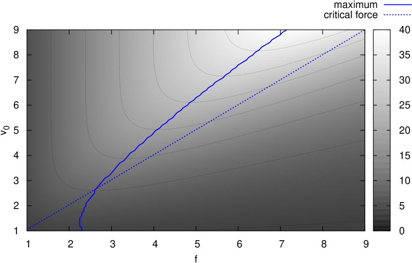
Figure 2: The ratio $\langle\dot{s}_{\mathrm{m}}\rangle/h(0)$ as a two dimensional contour plot for the parameters $f$ and $v_{0}$. The straight line is the critical force $f=v_{0}$. The thick line indicates the maximal value, i.e., it indicates the parameter pair for which the “kink” at $\sigma=0$ in Fig. 1 becomes the most pronounced.

A similar “kink” in the large deviation function around $\sigma=0$ can be observed for the analytically solvable asymmetric random walk. The asymmetric random walk is described by two rates $k^{+}$ and $k^{-}$ for a step forward and backward, respectively. The entropy produced or annihilated in a single jump is $b\equiv\ln(k^{+}/k^{-})$ Seifert (2005b, a). The random walker jumps $n^{+}$ steps forward and $n^{-}$ steps backward. The probability to have traveled $n\equiv n^{+}-n^{-}$ steps in the forward direction during a time $t$ is known analytically van Kampen (1981),

$$p(n,t)=I_{n}(2\sqrt{k^{+}k^{-}}t)(k^{+}/k^{-})^{n/2}e^{-(k^{+}+k^{-})t},$$ (13)

where $I_{n}(z)$ is the modified Bessel function of the first kind of order $n$. For the entropy production $s_{\mathrm{m}}=bn$, the generating function (3) becomes

$$\begin{split}g(\lambda,t)&\equiv\sum_{n=-\infty}^{\infty}e^{-\lambda bn}p(n,t)\\ &=e^{-(k^{+}+k^{-})t}\sum_{n=-\infty}^{\infty}I_{n}(z)\left[\sqrt{k^{+}/k^{-}}e^{-\lambda b}\right]^{n}.\end{split}$$

The sum can be evaluated using Abramowitz and Stegun (1972)

$$\sum_{n=-\infty}^{\infty}I_{n}(z)c^{n}=\exp\left[(z/2)(c+c^{-1})\right].$$

We thus obtain an exponentially decaying generating function $g(\lambda,t)=\exp[-\alpha_{0}(\lambda)t]$ with the single eigenvalue

$$\alpha_{0}(\lambda)=k^{+}\left[1+e^{-b}-e^{-\lambda b}-e^{-(1-\lambda)b}\right]$$ (14)

obeying the symmetry $\alpha_{0}(\lambda)=\alpha_{0}(1-\lambda)$ as expected . The curvature of the large deviation function $h(\sigma)$ at $\sigma=0$ can now be obtained analytically as

$$h^{\prime\prime}(0)=-\frac{[\alpha_{0}^{\prime}(0)]^{2}}{\alpha_{0}^{\prime\prime}(1/2)}=\frac{k^{+}}{2}e^{-(3/2)b}\left(e^{b}-1\right)^{2}.$$ (15)

For fixed forward rate $k^{+}$, this expression diverges for $k^{-}\rightarrow 0$ ($b\rightarrow\infty$), i.e., for vanishing backward steps.

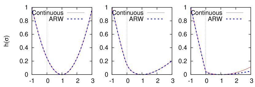
Figure 3: Comparison between the large deviation functions $h(\sigma)$ of the continuous dynamics and the asymmetric random walk (ARW). The parameters are: (left) $v_{0}=5$ and $f=0.05$, (center) $v_{0}=13$ and $f=1$, (right) $v_{0}=5$ and $f=4.05$.

In a parameter regime where the dynamics of the driven colloidal particle is dominated by hopping events from one potential minimum to another, i.e., for $f<v_{0}$, we can map the driven particle to the discrete asymmetric random walk. The escape rate $k^{+}$ can be obtained by specializing the general Kramers expression Hänggi et al. (1990) as

$$k^{+}=\frac{v_{0}}{2\pi}\chi\exp\left\{-2v_{0}[\chi-(\pi/2)a+a\arcsin a]\right\}$$ (16)

with $\chi\equiv\sqrt{1-a^{2}}$ depending on the two parameters $v_{0}$ and the ratio $a\equiv f/v_{0}$. In Fig. 3, we compare the large deviation functions of the continuous dynamics and the mapping to the corresponding asymmetric random walk for three different parameter sets $v_{0}$ and $f$. For small forces (left panel), the function $h(\sigma)$ is a parabola as it should be in such a linear response regime. Excellent agreement between the two models is also obtained for deep potentials and larger forces (center panel) for which $h(\sigma)$ significantly deviates from a parabola but still shows no “kink” at $\sigma=0$. Finally, in the right panel for $f$ approaching the critical force, the mapping to the Kramers model breaks down as expected. Still, both curves show a “kink” in this regime.

In summary, we have determined for a driven colloidal particle the large deviation function of the entropy production by calculating the lowest eigenvalue of the operator (9). We have used a numerical approach to directly calculate the eigenvalue without simulating trajectories. This approach can be extended to more complex systems with more than one degree of freedom through choosing an appropriate basis. We have further compared our results for a certain parameter range with a model where the large deviation function and the eigenvalue can be obtained analytically. In both cases, the large deviation function develops a “kink”, an abrupt change around zero entropy production. The question remains whether and to which extent this kink will be a general feature also present in interacting systems.

We acknowledge financial support from the DFG.

References

- Ellis (2006) R. S. Ellis, Entropy, Large Deviations, and Statistical Mechanics (Springer-Verlag, Berlin, 2006).
- Harris and Schütz (2007) R. J. Harris and G. M. Schütz, J. Stat. Mech.: Theor. Exp. p. P07020 (2007).
- Evans et al. (1993) D. J. Evans, E. G. D. Cohen, and G. P. Morriss, Phys. Rev. Lett. 71, 2401 (1993).
- Gallavotti and Cohen (1995) G. Gallavotti and E. G. D. Cohen, Phys. Rev. Lett. 74, 2694 (1995).
- Evans and Searles (2002) D. J. Evans and D. J. Searles, Adv. Phys. 51, 1529 (2002).
- Lebowitz and Spohn (1999) J. L. Lebowitz and H. Spohn, J. Stat. Phys. 95, 333 (1999).
- Kurchan (1998) J. Kurchan, J. Phys. A: Math. Gen. 31, 3719 (1998).
- Visco (2006) P. Visco, J. Stat. Mech.: Theor. Exp. p. P06006 (2006).
- van Wijland (2006) F. van Wijland, Phys. Rev. E 74, 063101 (2006).
- Ciliberto et al. (2004) S. Ciliberto, N. Garnier, S. Hernandez, C. Lacpatia, J.-F. Pinton, and G. R. Chavarria, Physica A 340, 240 (2004).
- Imparato and Peliti (2007) A. Imparato and L. Peliti, J. Stat. Mech.: Theor. Exp. p. L02001 (2007).
- Giardinà et al. (2006) C. Giardinà, J. Kurchan, and L. Peliti, Phys. Rev. Lett. 96, 120603 (2006).
- Lecomte and Tailleur (2007) V. Lecomte and J. Tailleur, J. Stat. Mech.: Theor. Exp. p. P03004 (2007).
- Faucheux et al. (1995) L. Faucheux, G. Stolovitzky, and A. Libchaber, Phys. Rev. E 51, 5239 (1995).
- Blickle et al. (2007) V. Blickle, T. Speck, C. Lutz, U. Seifert, and C. Bechinger, Phys. Rev. Lett. 98, 210601 (2007).
- Speck et al. (2007) T. Speck, V. Blickle, C. Bechinger, and U. Seifert, EPL 79, 30002 (2007).
- Seifert (2005a) U. Seifert, Phys. Rev. Lett. 95, 040602 (2005a).
- Seifert (2005b) U. Seifert, Europhys. Lett. 70, 36 (2005b).
- van Kampen (1981) N. G. van Kampen, Stochastic processes in physics and chemistry (North-Holland, Amsterdam, 1981).
- Abramowitz and Stegun (1972) M. Abramowitz and I. A. Stegun, eds., Handbook of Mathematical Functions (Dover, New York, 1972), 9th ed.
- Hänggi et al. (1990) P. Hänggi, P. Talkner, and M. Borkovec, Rev. Mod. Phys. 62, 251 (1990).