Results from an extensive simultaneous broadband campaign on the underluminous active nucleus M81*: further evidence for mass-scaling accretion in black holes

Abstract

We present the results of a broadband simultaneous campaign on the nearby low-luminosity active galactic nucleus M81*. From February through August 2005, we observed M81* five times using the Chandra X-ray Observatory with the High-Energy Transmission Grating Spectrometer, complemented by ground-based observations with the Giant Meterwave Radio Telescope, the Very Large Array and Very Large Baseline Array, the Plateau de Bure Interferometer at IRAM, the Submillimeter Array and Lick Observatory. We discuss how the resulting spectra vary over short and longer timescales compared to previous results, especially in the X-rays where this is the first ever longer-term campaign at spatial resolution high enough to nearly isolate the nucleus (17pc). We compare the spectrum to our Galactic center weakly active nucleus Sgr A*, which has undergone similar campaigns, as well as to weakly accreting X-ray binaries in the context of outflow-dominated models. In agreement with recent results suggesting that the physics of weakly-accreting black holes scales predictably with mass, we find that the exact same model which successfully describes hard state X-ray binaries applies to M81*, with very similar physical parameters.

1 Introduction

Black holes are a common feature in galaxies, spanning a huge range in mass, from the stellar-sized remnants scattered throughout the galaxy volume to the supermassive black hole often thought to lurk in the galaxy center. Black holes are known to operate over at least ten orders of magnitude in luminosity, and thus experience accretion rates that range from super-Eddington (defined with respect to an associated Eddington luminosity via $\dot{M}_{\rm Edd}\equiv L_{\rm Edd}/c^{2}$, where $L_{\rm Edd}\equiv{4\pi cGMm}/{\sigma_{\tau}}$) to extreme sub-Eddington. Clearly the accretion rate is the overall dominating factor determining the energy output; however, the accretion flow behavior of at least stellar mass black holes changes rather drastically between low to high accretion rates. Variations include the cyclic appearance and apparent subsequent quenching of jet outflows, alterations in accretion disk characteristics, and changes in the overall radiative efficiency. For a description of the most recent observations and their implications for theoretical models of accretion flows, see the reviews by Remillard & McClintock (2006); Done et al. (2007), and references therein.

Above a few percent of the Eddington luminosity, for instance, accretion around black holes seems to be well-characterized by a dominant, thermally emitting “standard thin disk” (Shakura & Sunyaev 1973). Somewhere below this threshold there appears to be a transition to a radiatively inefficient state with some form of advective accretion and/or outflow (see, e.g., Meyer & Meyer-Hofmeister 1994; Narayan & Yi 1994; Blandford & Begelman 1999; Quataert & Gruzinov 1999). Although this transition has been predicted theoretically, the physical details and configurations of weakly accreting flows are still under significant debate (see, e.g. Rykoff et al. 2007). In particular there are open questions regarding fundamental plasma characteristics such as the coupling– and therefore respective temperatures– of the ions and electrons, viscosity and the role of magnetic fields, the accretion flow geometry, and the relationship of the accretion flow to outflows and jet production.

For stellar mass black holes, we are learning a great deal by observing the transitions in real time between accretion states. Unfortunately, it is not possible to track such changes directly in supermassive black holes (SMBHs) as the relevant dynamical times scale approximately with the mass. Instead, ensemble comparisons can be made with large samples of accreting SMBHs that range from near-Eddington down to the intrinsically weakest active galactic nuclei (AGN), called low-luminosity AGN (LLAGN; Heckman 1980; Ho 1999). These sources are difficult to observe unless nearby, however, because of their intrinsically weak emission.

Given its special role as the weakest observable active nucleus, Sgr A*, our Galactic center SMBH, has become the poster-child for a multitude of theoretical and observational studies. Several extensive multiwavelength campaigns (e.g. Baganoff et al. 2003; Eckart et al. 2004; An et al. 2005; Yusef-Zadeh et al. 2006) have well established the simultaneous broadband spectrum of Sgr A*, which provides a tight constraint on physical models. Over the course of these campaigns, however, some very unusual flaring behavior has been discovered in Sgr A*’s X-ray emission. No other black hole has shown similar flaring; however, currently we are unable to detect any other Sgr A*-like objects for comparison. Furthermore, the presence of jets has not been definitively confirmed or ruled out for Sgr A*, complicating our ability to use it as a test source for accretion/outflow relationships at low accretion rates (but see Markoff et al. 2007). The distinct lack of any thin accretion disk component in its spectrum also makes Sgr A* unique compared to other LLAGN.

What seems to be required is a “bridge” source, to help span the gap between Sgr A* and other LLAGN in terms of accretion rate, while sharing as many other qualities as possible (mass, spectral features, galaxy type, etc.). Comparing Sgr A* to such a source would help us determine what processes may be different or absent at the lowest accretion rates. A comparison of this type, however, would require simultaneous broadband data for the bridge source, of the quality now only associated with the Galactic center campaigns.

The nucleus of the nearby galaxy M81 is an ideal candidate for such an extensive multiwavelength campaign on a LLAGN, for the following reasons. Although it is one of the intrinsically weakest LLAGN known, it is among the brightest because it is the nearest galaxy besides Centaurus A with a central AGN. Furthermore it is the nearest point-like LLAGN, similarly inside a spiral galaxy, for which reliable measurements of the black hole mass are available. Spectroscopy with the Hubble Space Telescope (HST) suggests a central mass of $7\times 10^{7}$$\rm\thinspace M_{\odot}$ (Devereux et al. 2003), and M81’s distance is only 3.6 Mpc (Freedman et al. 1994). The nucleus, M81* (following the convention based on Sgr A*), is associated with a compact radio core and exhibits both low-ionization emission line region (LINER; Heckman 1980; Ho 1999) and Seyfert 1 characteristics. In terms of radiative power, probable accretion rate, and the length of the jet emanating from the core, M81* lies in the intermediate range between radio loud AGN and Sgr A*.

The X-ray properties of M81* are very typical for the LLAGN class (e.g. Ho 1999). Its nonthermal X-ray luminosity is around a few $10^{-5}L_{\rm Edd}$, though its proximity means it is still bright. Similarly its spectral energy distribution (SED) displays no “big blue bump” yet does show evidence for double-peaked optical line emission (Bower et al. 1996), suggesting the presence of a weak accretion disk. HST observations with STIS indicate that the disk is close to face-on with an inclination of 14^∘ (Devereux et al. 2003).

As will be described in more detail below, M81* exhibits significant variability across its SED on both short (daily) and long (monthly/yearly) time scales. M81* has a low absorption column (Page et al. 2003), which allows UV and soft X-ray detection. Perhaps most importantly for the goals of this campaign, M81* shares several important characteristics with Sgr A*, specifically its radio slope and polarization, that make it the ideal comparison source. As studies of our own Galactic center have shown, detailed, multi-wavelength observations of single objects such as M81* are indispensable tools for understanding black hole accretion.

In this paper we will present the results of a simultaneous, broadband, multiwavelength campaign on M81*, and discuss how it compares with Sgr A*, as well as its weakly accreting black hole counterparts in X-ray binaries (XRBs). The Chandra observations specifically resulted in the first gratings-resolution X-ray spectrum of an isolated LLAGN nucleus, which is the focus of a companion paper (Young et al. 2007). The millimeter observations carried out with the Plateau de Bure Interferometer(PdBI) are also presented in more detail elsewhere (Schödel et al. 2007). In Section 2 we summarize the results of previous observations of M81* and in Section 3 we describe our new observations and analysis. We present the resulting broadband spectra in Section 4 and their interpretation in the specific context of a jet-dominated model in Sections 5 & 5.3. Section 6 contains our discussion and conclusions.

2 Previous Observations of M81*

The M81* nucleus has been observed extensively in many wavebands (partly due to its proximity to supernova SN 1993J, which undergoes regular monitoring). In this section we will briefly summarize the previously known broadband characteristics of M81* and discuss how they have provided the motivation for more detailed and higher resolution observations.

2.1 Radio/millimeter Observations

M81* exhibits the signature flat/inverted radio spectrum associated with the compact cores of AGN. Such a spectrum is well-explained by a collimated, steady jet which radiates via self-absorbed synchrotron emission along its length (see, e.g. Blandford & Königl 1979; Falcke 1996). Based on observations from 1.4–22.5 GHz using the VLA, several groups have observed an inverted spectrum ($\alpha\sim 0.0$–0.3, $F_{\nu}\propto\nu^{\alpha}$) with a flux in the range of $\approx 80-300$ mJy (Ho et al. 1999; Bietenholz et al. 2000; Brunthaler et al. 2001, 2006). Based on four years of observations with the VLA, Ho et al. (1999) note that M81* undergoes frequent radio outbursts, with the underlying flux around $100$ mJy and higher fluxes during flares. The larger flare events occur on time scales of months, and seem to roughly correspond with predictions of simple adiabatic expansion models (e.g. van der Laan 1966) in which the variability moves towards lower frequencies as the flare amplitude decreases. Ho et al. also claim they detect intraday variability at a level of 10-60% amplitude changes. If the longer term radio flares are indeed expanding ejecta moving out along otherwise steady jet structures, there should be even higher amplitude variations in the millimeter regime. Consistent with this view, Sakamoto et al. (2001) observed the 3 mm flux to double within a single day.

A one-sided jet system has been resolved in M81*. Bietenholz et al. (2000) identified a stationary radio core with a very small (700 AU at 22 GHz), precessing (over 20^∘) jet, the structure of which varies on relatively short timescales. Interestingly, this group found no significant intraday variations over a similar time frame as the Ho et al. study. Investigating this question of variability was one of our campaign’s goals for the lower frequencies.

M81*’s radio luminosity is about four orders of magnitude brighter than Sgr A*’s, but its shape and polarization are quite similar. A key, and somewhat unusual, trait that these two sources share is the dominance of circular polarization up to $\mathrel{\hbox to0.0pt{\raise 2.20013pt\hbox{$>$}\hss}{\lower 2.20013pt\hbox{$\sim$}}}22$ GHz in M81*, and $\sim 112$ GHz in Sgr A* (Brunthaler et al. 2001; Bower et al. 2002; Brunthaler et al. 2006). Sgr A* becomes increasingly linearly polarized towards its peak flux in the submm (Bower et al. 2003, 2005); however, the characteristics of M81* in the submm have not yet been determined. The interpretation of Sgr A*’s circular polarization is Faraday depolarization by the surrounding accretion flow. If the same physics is active in M81*, we would expect to detect linear polarization in the submm range as well.

2.2 Infrared through Ultraviolet Observations

Typical of LLAGN, M81* lacks a bright optically thick “standard thin disk” component in the optical range, although double-peaked optical lines do suggest the presence of a weak disk (Bower et al. 1996). The low column ($N_{h}\sim 5\times 10^{20}$ cm^-2; Page et al. 2003) allows us to detect UV and soft X-rays from the nucleus, which suggests a nearly face-on disk. Maoz et al. (2005) used the HST ACS to discover variable (by tens of %) UV emission, consistent with the results of Ho et al. (1996), who detected a weak and very steep ($\alpha\approx-2$) UV continuum. Instruments with less spatial resolution such as Spitzer (Willner et al. 2004; Murphy et al. 2006), MIRLIN (Grossan et al. 2001) and ISOPHOT-S (Satyapal et al. 2005) are all consistent with a steep ($\alpha\leq-1.7$) non-stellar spectrum, similar to what is observed in the IR/UV in the LLAGN NGC 4258 (Chary et al. 2000). This is of interest because it suggests that in LLAGN, the UV is likely nonthermal emission, while the optical, and perhaps IR, contain the only potential signatures of a radiatively efficient, thin accretion disk.

2.3 X-ray Observations

M81* has a persistent nonthermal power-law flux in the X-rays, with variations of factors of 3 or more over yearly time scales. ASCA has detected both long term variations, as well as 20–30% intraday variations which suggest that the source size is less than a few hundred gravitational radii ($r_{\rm g}\equiv GM/c^{2}$) (Iyomoto & Makishima 2001). ROSAT also confirmed long term X-ray variability, with a factor of $\approx 2.5$ amplitude (Immler & Wang 2001). A summary of these and more recent variability trends can be found in La Parola et al. (2004). M81*’s X-ray luminosity appears to vary between ($2$–$6)\times 10^{41}$ ergs s^-1, which corresponds to $\sim(2$–$6)\times 10^{-5}L_{\rm Edd}$. It was not until observations with BeppoSAX that more detailed statements could be made about the nuclear X-ray emission properties. Pellegrini et al. (2000) observed both the short intraday as well as the long term variability over the 0.1–100 keV band. However, due to the poor angular resolution, they could only place a lower limit of $\mathrel{\hbox to0.0pt{\raise 2.20013pt\hbox{$>$}\hss}{\lower 2.20013pt\hbox{$\sim$}}}80\%$ of the continuum originating in the nucleus.

The BeppoSAX observations yielded several important new results which contributed to our interest in M81* as a potential Chandra HETGS target. First, the data were consistent with no reflection component or blue bump, which would be unusual for a Seyfert 1 – a class of objects with which M81* otherwise shares some qualities. The BeppoSAX results make it less likely that M81* is a simple extension of the Seyfert 1 class to low luminosity. Although BeppoSAX did not detect reflection, it did detect emission and absorption features of highly ionized iron; however, these features were seemingly not correlated with the continuum luminosity. Second, there were problems reconciling the ionization with the low inferred accretion rate. Pellegrini et al. (2000) suggested that instead of ionization, there may instead be transmission through a highly photoionized medium close to the nucleus, such as a warm absorber. Third, while the observed X-ray powerlaw with $\Gamma\approx 1.8$–1.9 was typical of bright Seyferts, there was no direct evidence for a thin accretion disk. A lack of a strong disk component is consistent with accretion being dominated by a radiatively inefficient accretion flow (RIAF); however, the question then arises whether such flows can account for the strong Seyfert-like powerlaw over the entire 0.1-100 keV range at the low inferred accretion rates of M81*. XMM-Newton has confirmed these findings, at least in the 0.3-8 keV band, and also detected redshifted Fe K$\alpha$ as well as He- and H-like ionized iron (Page et al. 2003).

Because Chandra is the only X-ray mission with the spatial resolution to almost isolate the nucleus of M81* (to within $\sim 17$ pc of the black hole), determining the nature of the line emission was one of our primary goals. As described in Young et al. (2007), we indeed detect not just iron but many other low-metallicity species, as well as velocity broadening of some of these lines. The broadened line components are consistent with arising from regions close to the black hole, i.e., $\mathrel{\hbox to0.0pt{\raise 2.20013pt\hbox{$<$}\hss}{\lower 2.20013pt\hbox{$\sim$}}}10^{5}~{}GM/c^{2}$. Detected line features include those associated with fluorescence from cold material (Ar K$\alpha$, Si K$\alpha$, and Fe K$\alpha$), emission lines from a hot plasma (Ne x, Mg xii, Si xiii), and absorption lines (18.44 Å and 20.74 Å) that could be consistent with an outflowing wind. The plasma emission lines, specifically the Si xiii triplet line strength ratios, are consistent with a collisionally ionized plasma (although other models can not be ruled out). The focus of the Young et al. (2007) work is on the X-ray spectra of M81*, specifically the aforementioned line features in relation to the X-ray continuum. Young et al. show that the X-ray spectra are consistent with the expectations of a somewhat simplified RIAF model. We did not consider the simultaneous radio and submm data in the context of those models. In this work we now include a description of the lower frequency (radio through sub-millimeter) observations, and consider the entire broadband spectrum in the context of an outflow-dominated model.

3 Observations and Data Reduction

The difficulty in observing a source as faint as M81* with the Chandra HETGS lies in the required long integration times (300 ksec) to adequately resolve the narrow ($\mathrel{\hbox to0.0pt{\raise 2.20013pt\hbox{$<$}\hss}{\lower 2.20013pt\hbox{$\sim$}}}2500~{}{\rm km~{}s^{-1}}$ Full Width Half Maximum) line features. Additionally, aside from the Fe features found with BeppoSAX and XMM observations (which, due to the relatively poorer spatial resolution of these instruments, could have arisen from well outside the nucleus), the existence of line features from the innermost regions of LLAGN was uncertain. As such, at the time of our M81* observations, no gratings observation of an LLAGN had been accepted in the Chandra Guest Observer program. Instead, we obtained a series of HETGS observations via the Guaranteed Time Observation program (PI: C. Canizares). In order to further constrain models and better understand the variability trends of M81*, we supplemented the Chandra program by proposing for simultaneous coverage with five ground-based instruments that span the lower frequencies: the Giant Meterwave Radio Telescope (GMRT), the Very Large Array/Very Large Baseline Array (VLA/VLBA), the Plateau de Bure Interferometer (PdBI) at IRAM, the Sub-millimeter Array (SMA), and Lick Observatory.

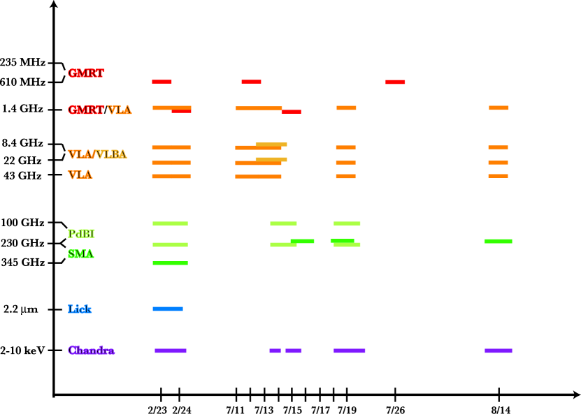
Figure 1: Schematic overview of the entire campaign during 2005.

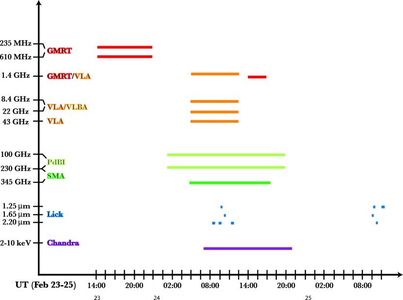
Figure 2: Schematic overview of the 2005 February 23–25 period. Exact times are shown in Table 1.

Figure 1 gives an overview of the total campaign. For the two periods of greatest multi-wavelength overlap, Figures 2 & 3 give a closeup view of the coverage, and Tables  1– 4 give the exact times in UT.

In the following subsections we provide details of the individual instrument observations and data reduction.

3.1 Low-frequency Radio Waves: GMRT

The Giant Meterwave Radio Telescope (GMRT) is an aperture synthesis radio telescope (Swarup et al. 1991) situated 80 km north of Pune in Western India at latitude $19^{o}\,06^{\prime}$ and longitude $74^{o}\,03^{\prime}$ E. The telescope operates at 233, 327, 610 and 1420 MHz bands, and consists of 30 fixed position, fully steerable paraboloid dishes of diameter 45 meters. Fourteen out of these 30 dishes are located within about a square kilometer of each other, the remaining 16 antennae form a “Y”-shaped array with northwest, northeast and southern arms spread over an area of 25 kilometers in diameter. The baselines in the central one square kilometer area are useful to map the extended emission of the source, whereas the wider baselines in the “Y” provide high angular resolution.

We observed M81* with the GMRT in 1420, 610 and 235 MHz bands on several occasions during the campaign. The total time spent on M81* in the 235/610 bands was 5–8 hours, and 3–5 hours in the 1420 MHz band. The bandwidth at 1420 and 610 MHz was 16 MHz, divided into a total of 128 frequency channels, i.e., the default for the correlator. For the 243 MHz wave band the bandwidth was 6 MHz.

Calibrator sources were used to remove the effects of instrumental variations in the measurements. 3C48, 3C286 and 3C147 were used as flux calibrators. 1035+564 was used as a phase calibrator in the 1420 MHz observations, whereas 0834+555 was used in the 610 and 235 MHz observations. The flux and phase calibrators were used for bandpass calibration as well. Flux calibrators were observed once or twice for 20–30 minutes during each observing session. Phase calibrators were observed for 5–6 minutes after every 25 minutes of observations.

We used the Astronomical Image Processing System (AIPS) developed by NRAO for the data analysis, including the standard GMRT data reduction (see Chandra et al. 2004, for details). Standard flagging routines of AIPS were used to remove the bad antennas and corrupted data. About 25–30 antennae could be used in the radio interferometric setup at different observing epochs. Data were then calibrated and images and fields were formed by Fourier inversion and CLEANing using AIPS task IMAGR. We took into account the bandwidth smearing effects and wide field imaging, even though in this case M81* is not spatially resolved, as a byproduct of analysis to derive the correct flux density of the nearby SN 1993J. Bandwidth effects were negligible for 1420 and 610 MHz bands and we averaged 100 central channels. For the 235 MHz observations, we divided the central 55–60 good channels and divided them into 4 sub-bands and stacked them together while imaging. To take care of the wide field imaging, we divided the whole field in 3 subfields for 1420 MHz and 610 MHz observations, and into 18 subfields for 235 MHz observations. A few rounds of self-calibrations were also performed in all the datasets to remove the phase variations. AIPS task FLATN was used to combine all the sub fields into one single image. Table 5 gives details of the observations. The typical resolution of $3"$ at 1390 MHz at a distance of 3.6 Mpc for M81 corresponds to about 54 pc. Table 6 shows a comparison of calibration observations of SN 1993J for both the GMRT and the VLA, indicating consistent flux levels.

3.2 Centimeter Radio:
VLA and VLBA+Effelsberg

The Very Large Array observed M81* on 2005 14 February, 13 July, 19 July, and 14 August. Observations were obtained at 1.4, 8.4, 22, and 43 GHz on each of the days in continuum mode. Data were obtained in fast-switching mode between M81* and the compact calibrators J1048+717 and J1056+701. We performed calibration of amplitude and phase variations on short time-scales using J1048+717 and transferred solutions to M81* and J1056+701. Results for J1056+701 are, therefore, a check on variability of M81*. The amplitude scale was set by observations of 3C 286. Weather on 14 February and 13 July was poor making results at 22 and 43 GHz inaccurate. We determined average flux densities for each day as well as measuring flux density on short time scales. SN 1993J was in the field of view at 1.4 and 8.4 GHz. Its flux density was constant between the epochs.

The Very Long Baseline Array and the Effelsberg 100m observed M81* on 2005 13 July. Observations were made at 8.4 GHz with a sampling rate of 128 Mb/s, while attempts at 22 GHz failed due to poor weather. Standard self-calibration reduction techniques were performed and M81* was imaged with a resolution of 0.6 mas. M81* is clearly resolved into a compact and extended component (Fig. 4). The peak flux density in the compact component is about 60 mJy. In the extended component, the peak flux density is about 10 mJy, but the total flux density in the whole region is $\approx 2$–3 times that value. We fit the image with two elliptical Gaussians: the best fit compact component has major axis of 0.65 mas, a minor axis of 0.57 mas and a position angle of 81^∘, and the best fit extended component has major axis 1.5 mas, minor axis 0.66 mas and position angle 55^∘. The separation between the two components is approximately 1 mas, and the total extension is about $10^{4}$ AU across. These results are similar to what was observed by Bietenholz et al. (2000).

Our results are summarized in Table 7. We obtained limits on the linear polarization on 2005 13 July of 0.1% at all frequencies, but did not obtain accurate limits on the circular polarization of the source.

3.3 Millimeter Radio: PdBI

The continuum radiation from M81* at wavelengths of $\sim$3 mm and $\sim$1 mm was observed with the IRAM Plateau de Bure Interferometer (PdBI) on 2005 24 February, 14-15 July, and 19-20 July. The observation frequencies differ slightly between the individual epochs because they were fine-tuned in order to optimize phase stability depending on the weather conditions. A detailed description of the data, their reduction and calibration can be found in Schödel et al. (2007). The systematic absolute uncertainty of the flux calibration is 10-15% for the 3mm data, and 15-30% for the 1mm data (see Table 2 in Schödel et al.). Flux measurements were extracted from individual scans of 20 min duration and detailed light curves were obtained that show significant variability of M81* during the observations. If we add the systematic uncertainties with the statistical uncertainties in quadrature,the resulting overall uncertainty is around 20% (3mm) and 30% (1mm). Because the detected flux variations are likely real,and fully consistent with what is observed in other wavebands, including the systematics in this manner would seem to overestimate the actual uncertainties. For this reason we believe that taking the standard deviation of the flux is more representative of the total uncertainty in the context of this broadband system. For this reason we use the average fluxes and their standard deviations as obtained from the light curves presented in Schödel et al. (see their Table 3), which we list in Table 8.

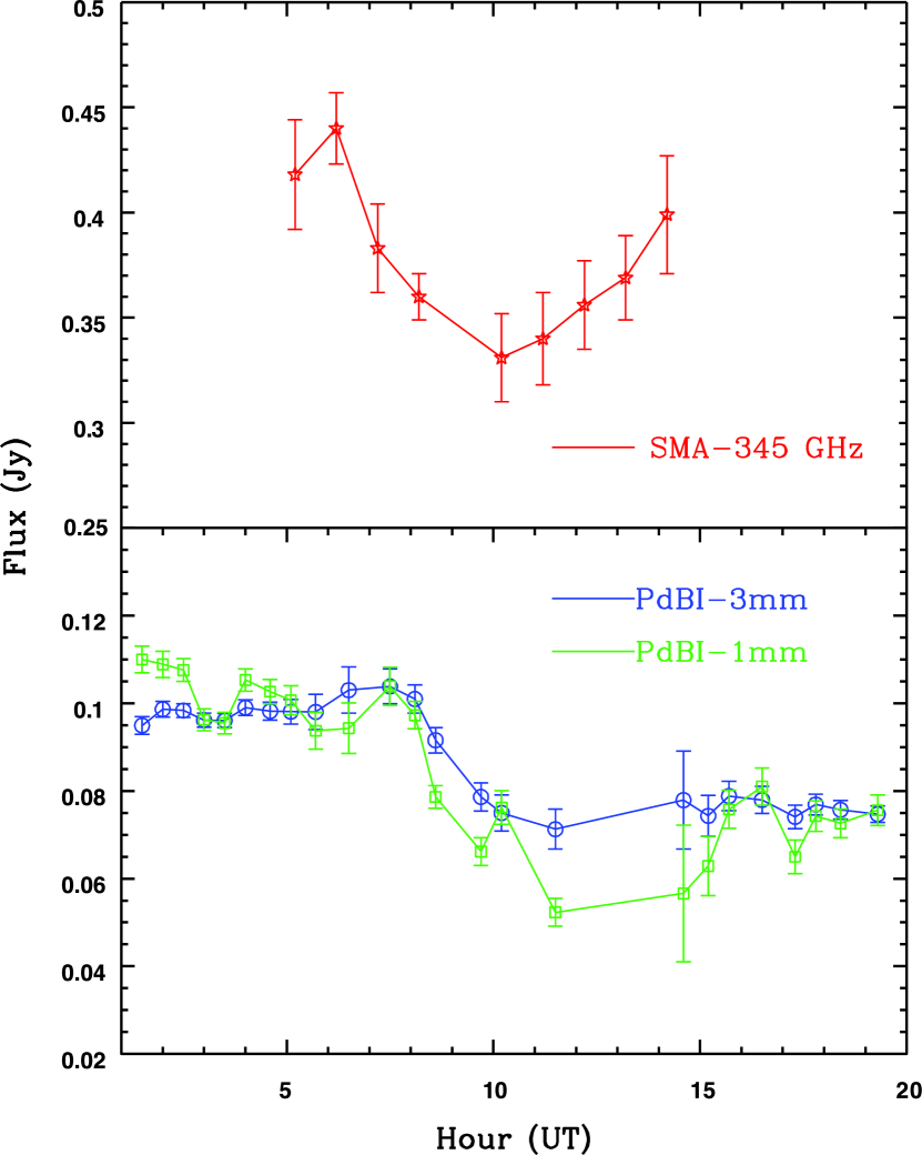
Figure 11: Comparison of PdBI and SMA lightcurves from 24 Feb.

The PdBI observed significant variability between the individual observing epochs, as well as intraday variability. The 3mm and 1 mm light curves from 2005 24 February — actually the best of the data obtained with the PdBI during the campaign — show a flux decrease with a significance of $>5\sigma$ over 5 hours that occurred at both wavelengths (see Schödel et al. 2007 for a detailed discussion). The lightcurves are presented in combination with those from the Submillimeter Array below in Figs. 11 & 12.

3.4 Submillimeter: SMA

M81* was observed at the Submillimeter Array (SMA; Ho et al. 2004) on Mauna Kea on 2005 Feb 24, 2005 Jul 18 and 2005 Aug 14. Observations were also made on 2005 Jul 15, but the daytime phase stability was too poor to permit reliable calibration of the data. In all cases, 7 of the 8 SMA antennas were available. The observations on 2005 Feb 24 were made in good nighttime winter conditions, with optical depth towards zenith at 225 GHz $\tau_{225}\sim$0.04 and 10% humidity. The summer observations suffered somewhat from afternoon atmospheric turbulence, and were made with $\tau_{225}\sim$0.05 and 40% humidity on 2005 Jul 18, and $\tau_{225}\sim$0.12 and 20% humidity on 2005 Aug 14.

The SIS receivers were tuned to a center frequency of 345.796 GHz in the upper sideband for 2005 Feb 24, and 230.538 GHz in the upper sideband for 2005 Jul 18 and 2005 Aug 14. For the initial observations on 2005 Feb 24, one IF was configured with a higher spectral resolution to search for CO(3-2) at the systemic velocity of M81, but none was detected. This is consistent with the absence of CO(1-0) emission at the position of the core reported by Sakamoto et al. (2001). For all observations, the full 4 GHz (2 GHz in each sideband separated by 10 GHz) were averaged to construct one continuum channel centered on 340.67 GHz and 225.42 GHz, respectively.

The SMA data were calibrated using the MIR software package developed at Caltech and modified for the SMA. Gain calibration was performed using the nearby quasar 0958+655. Absolute flux calibration was performed using Callisto, and at least 2 of the following quasars– 0721+713, 0841+708, 0927+390, 1153+495– were observed hourly to ensure that any detected changes in the flux of M81* were real, and not an artifact of the calibration. This is particularly important for the summer observations, which were made under poorer daytime conditions. The data were imaged using difmap to confirm that M81* is unresolved at the 1$.\!\!^{\prime\prime}$5-3$.\!\!^{\prime\prime}$0 resolution of the SMA, following which the fluxes of both M81* and the nearby quasars were determined by fitting a point source model to the data in the ${u,v}$ plane. The flux densities obtained are accurate to within 20%, based on the derived values for the quasars.

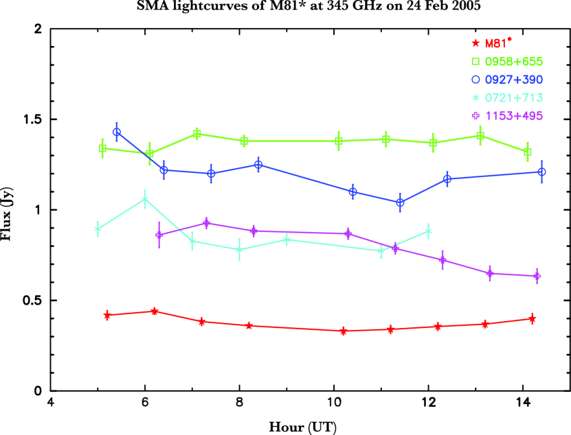
Figure 8: Lightcurve of 24 Feb SMA observations of M81* and calibrators.

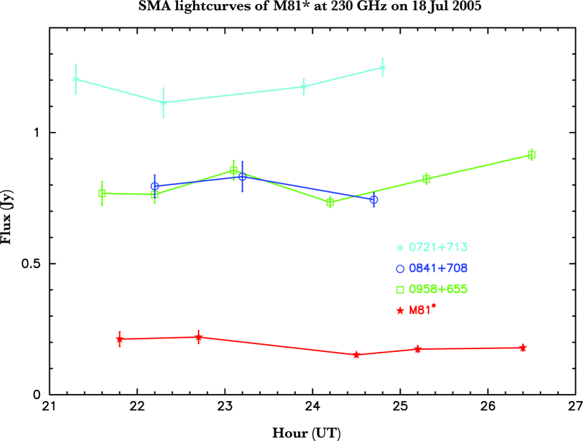
Figure 9: Lightcurve of 18 July SMA observations of M81* and calibrators.

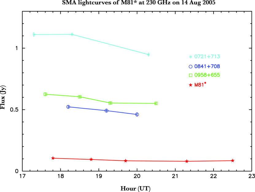
Figure 10: Lightcurve of 14 Aug SMA observations of M81* and calibrators.

As shown in Figs. 8–10, M81* exhibited little to no variation on short timescales during the observations, although there may have been a brief dip in flux in the February data shortly preceding the apparent corresponding dip in the PdBI measurements shown in Fig. 11. This dip should be viewed with caution, given that the level of variation is not greater than the random variations seen in the calibrators, however the shape and timing are suggestive. More significant variations in flux were seen between the epochs, as shown in Fig. 12.

The average flux on 2005 Feb 24 was 378.7$\pm$70.0 mJy at 340 GHz. For 2005 Jul 18 and 2005 Aug 14, we obtained 182.8$\pm$36.0 mJy and 91.5$\pm$15.3 mJy at 225 GHz, but it should be noted that the August data were obtained in substantially worse weather, with higher atmospheric opacity in addition to the normal summer daytime turbulence, and so the phase transfer from 0958+655, although only 4 degrees away, may not have been entirely successful, resulting in a lower flux density within a point source model.

3.5 IR: Lick Observatory

We observed M81^∗ with the infrared camera for adaptive optics at Lick (IRCAL) behind the laser-guide star adaptive optics (LGSAO) system on the Shane 3 m telescope on the nights of 2005 February 24 and 25 (see Tab. 1 and Figs. 1 and 2). In the near-infrared, M81^∗ is an unresolved point source on top of a bright, extended background from the stars and gas in the nuclear regions. The high galactic background made use of the laser guide star necessary; attempts to use the bright nucleus as a natural guide star for AO correction failed.

We cycled through observations in the $J$, $H$, and $K_{\rm s}$ bands, with more time spent on the $K_{\rm s}$ band where the correction is best. For each cycle a 5-point dither pattern was repeated twice. Each frame in the dither pattern was 50–90 s long in the $J$ band, 60 s long in the $H$ band, and 60 s long in the $K_{s}$ band. We created flats by taking the median of a series of images of the telescope dome with the lights turned on, and divided each frame by the flat. We then subtracted the sky background from each frame using a nearby, relatively blank field. The sky background was small compared to the bright extended emission from the galaxy.

Co-added images were created by shifting and adding the images from each 5-point observing pattern. The shifts between the dithered images were empirically determined between frames using the centroid of a 2-dimensional Gaussian fitted to the emission from M81^∗ before summing the frames. Frames with an average $\sigma>11.2$ pixels (0$.\!\!^{\prime\prime}$85) were excluded; this cutoff value was determined empirically by plotting the peak pixel value versus the average $\sigma$ for each frame. (This average $\sigma$ value is from a single Gaussian fit to the extended galaxy plus M81^∗.) Co-added images were then divided by an exposure map with the total exposure time per pixel to create fluxed images in units of counts sec^-1.

Each night we obtained two images of a nearby star (GSC 04383–00224) in order to test the stability of the point-spread function (PSF), and these images revealed the PSF to be variable. For instance, in the $K_{s}$ band, the best PSF image was nearly diffraction-limited with a half-width half-maximum (HWHM) of 0$.\!\!^{\prime\prime}$17, but the poorest on the same night had a HWHM of 0$.\!\!^{\prime\prime}$25. No other point source was detected in the 20^′′ field of view of M81^∗ that would allow us to track the shape of the PSF concurrent with each exposure, and we found that without empirical knowledge of the PSF we were unable to construct a self-consistent model of the light from the galaxy and the active nucleus. This prevented us from obtaining accurate point-source photometry of the nucleus, and thus constraining any variability. Therefore, we computed an upper limit to the $K_{s}$ band nuclear flux averaged over the course of the observations.

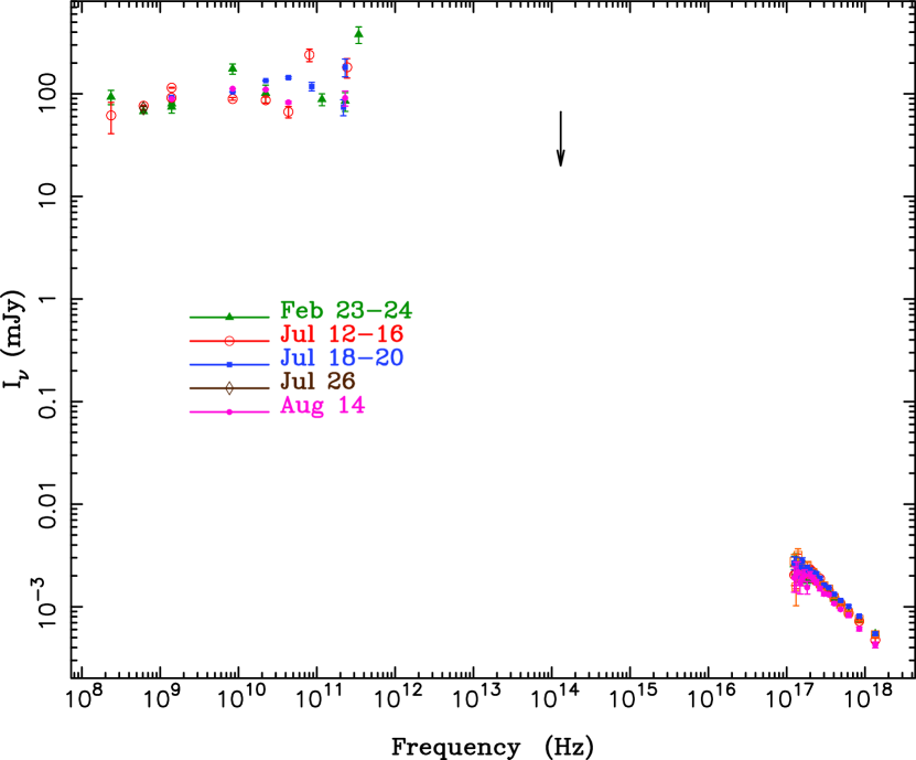
Figure 5: The combined spectral energy distribution from all observations in the 2005 campaign. (Dates are labeled in different colors for the electronic version.) The base of the arrow represents the upper limit established by Lick, while all other points represent actual detections with estimated errors. X-ray data are for the MEG $\pm 1^{\rm st}$ order spectra (combined).

To determine the upper limit, we measured the radial profile of the PSF calibration star, GSC 04383–00224, and used its 2MASS $K_{\rm s}$ magnitude to determine the photometric zeropoint for converting from counts to magnitudes using a large aperture (30 pixels = 2$.\!\!^{\prime\prime}$28). At radii larger than 30 pixels, the background-subtracted, enclosed counts change by $<2\%$ while the noise increases. Given that M81^∗ lies on top of strong extended emission from the galaxy, we preferred to use a smaller aperture of 10 pixels (0$.\!\!^{\prime\prime}$76) with the aperture correction determined from the calibration star; a 10-pixel radius circle encloses 79% of the counts within a 30-pixel aperture. The local background was estimated from the median in an annulus with inner radius of 30 pixels and outer radius of 40 pixels (3$.\!\!^{\prime\prime}$04) and subtracted; this likely underestimates the true local background as the extended galaxy emission is also peaked at the position of M81^∗. The calibration star photometry, measured at three different airmasses (1.20, 1.32, and 1.36) was also used to calculate the local $K_{\rm s}$-band atmospheric extinction correction. Following this procedure, we found an upper limit value of 66.7 mJy in $K_{\rm s}$. This limit is displayed as the base of the arrow in Figure  5.

3.6 X-rays: Chandra

M81* was observed by the Chandra X-ray observatory, with the High-Energy Transmission Grating Spectrometer (HETGS; Canizares et al. 2005) in place, on five separate occasions (see Tables 1–5). The HETGS consists of two sets of transmission gratings, the High Energy Gratings (HEG) covering the 0.8–10 keV bandpass with a spectral resolution of $\Delta\lambda=0.012$Å FWHM, and the Medium Energy Gratings (MEG) covering the 0.4–8.0 keV bandpass with a spectral resolution of $\Delta\lambda=0.023$Å FWHM. The angular resolution of Chandra, even with the insertion of the gratings, isolates X-ray emission from the central $<1\hbox{${}^{\prime\prime}$}$ around M81*. We do not utilize information from the $0^{\rm th}$ order (undispersed) spectrum, however, as the central image of the nucleus suffers from photon pileup (Young et al. 2007).

The Chandra data were filtered for times of high background and spectra were extracted using the standard CIAO tools, using v3.3 of the software and CALDB 3.2.2. Analyses were performed using ISIS version 1.4.7 (Houck 2002). Our data preparation was identical to that described in Young et al. (2007). Specifically, for all X-ray analyses we separately combined the $\pm 1^{\rm st}$ HEG spectra and the $\pm 1^{\rm st}$ order MEG spectra, and we utilized background files from narrow regions on either side of the respective gratings arms. As discussed in Young et al. (2007), we are confident that $\mathrel{\hbox to0.0pt{\raise 2.20013pt\hbox{$>$}\hss}{\lower 2.20013pt\hbox{$\sim$}}}90\%$ of the dispersed X-ray emission originates in an unresolved source in the nucleus of M81.

4 Observational Results

4.1 The Broadband Spectrum of M81*

Figure 5 shows the broadband spectrum comprised of all of our observations from the 2005 campaign. It is immediately clear that while there was some variability, particularly in the radio to mm, we did not see large variations in the X-ray or overall basic shape of the SED. The total average 7 GHz radio luminosity is $L_{\rm R}=8.2\times 10^{36}$ erg s^-1 and the total average 2–10 keV X-ray luminosity is $L_{\rm X}=1.52\times 10^{40}$ erg s^-1. The radio exhibited $\approx 20$% variation about this average while the X-rays exhibited $\approx 14$% variation. Therefore over the course of this half-year campaign, M81* appeared to be more stable in both wavebands than has been reported in the past. Interestingly, however, the average $L_{\rm R}$ seen in our campaign is $\approx 25$% lower than the average deduced from all prior campaigns, while our average $L_{\rm X}$ is about a factor of 5 less (see Markoff 2005). Either we have caught M81* in a rather low, stable state, or previous observations (with notably larger fields of view) have included a large flux contribution from the surrounding diffuse medium.

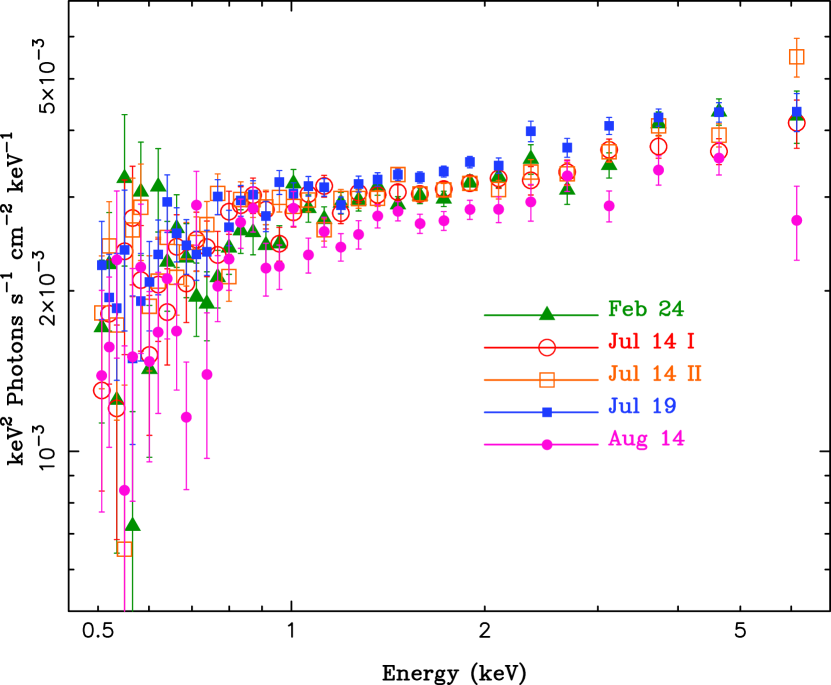
Figure 6: Flux density ($\nu L_{\nu}$) of the X-ray band for all observations during the campaign (in color for the electronic version). The slope for all observations is well-fit by a power-law of photon index $\Gamma\approx 1.75$–1.85. The largest change in continuum was between July 19 and August 14, with a drop of $\approx 20$% within a month.

Fig. 6 shows the flux density for all X-ray observations, where we see that the largest change was a drop between July and August. The 2005 July 19 observations with the HEG showed a 0.8-7 keV flux of $1.31\pm 0.02\times 10^{-11}~{}{\rm erg~{}cm^{-2}~{}s^{-1}}$— the highest value during our campaign— while the 2005 August 14 observations with the HEG dropped down to a value of $1.07\pm 0.03\times 10^{-11}~{}{\rm erg~{}cm^{-2}~{}s^{-1}}$. (See Young et al. 2007 for further discussions of the X-ray variability.)

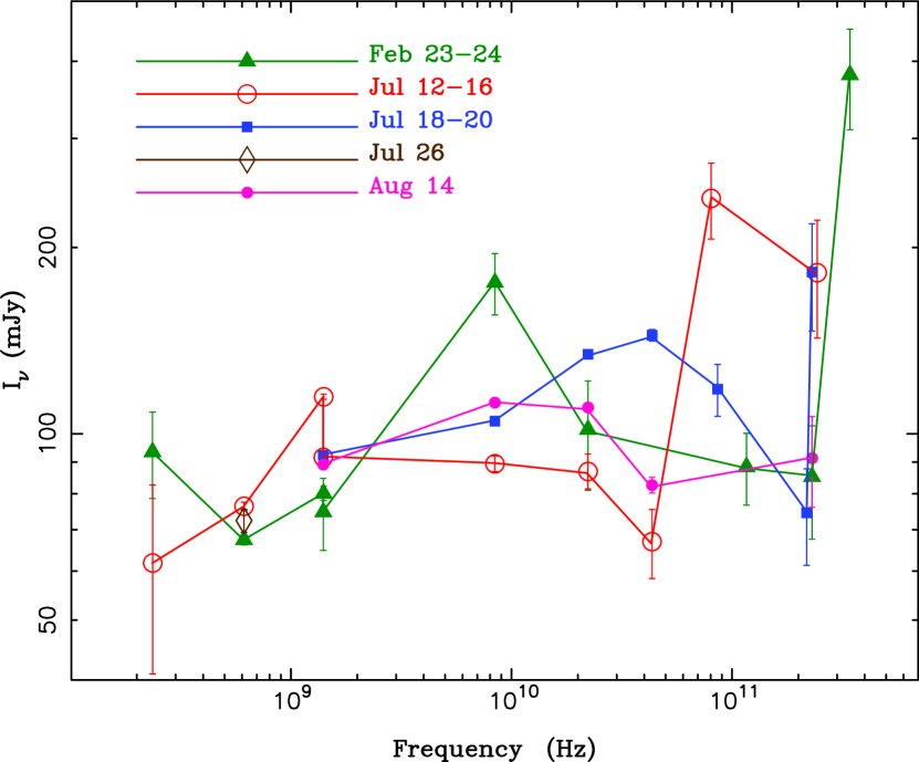
Figure 7: Spectral energy distribution of the centimeter through submm observations from the campaign (in color in the electronic version). Note the significant variability, especially at the higher frequencies. We detect significant intraday variability during both 2005 February and July, as well as apparent waves moving lower in frequency and amplitude consistent with adiabatic expansion of blobs in a jet.

The radio through submm bands revealed significantly more variability in comparison to the X-ray band. Fig. 7 shows the good data for all observations. The most reliable detection of significant intraday variability occurred at 3mm and 1mm in the PdBI observations on 24 February. A flux decrease of $\sim 30$% with a significance of over $5\sigma$ was observed in both bands from 08h to 12h UT (see Fig. 11 and Schödel et al. 2007). Such a time scale would suggest that the size of the emitting region is less than 20 $r_{\rm g}$, if beaming were not involved. The expected beaming from our spectral fits discussed below is mild for the weak jet in this LLAGN; therefore, the mm variability still implies a relatively compact source.

The SMA observations were successful in the 345 GHz band only on the first observing run in February. The resulting spectrum shows a suggestive upturn towards the submm (Fig. 7, 15). This steepening is similar to the spectral component seen in Sgr A* that is referred to as the “submm bump”. In Sgr A*, this bump rapidly declines with decreasing wavelength towards the infrared (IR), and furthermore it varies simultaneously with the X-rays (Eckart et al. 2004, 2006a). This simultaneous variation suggests that for Sgr A* the IR and X-ray emission both originate in regions close to the SMBH. In contrast, the variability detected in M81* is both less pronounced and not as clearly correlated between the submm and X-ray.

That being said, however, the low-frequency data are suggestive of waves of variability, with decreasing amplitudes, that appear to be moving from shorter to longer wavelengths over the half year of monitoring. Specifically, note that the peak at just under 10 GHz in 2005 February is gone by 2005 August, and does not appear to be associated with any lower frequency features. (The “peak” in the 2005 July 12-16 at just above 1 GHz is a mismatch between the GMRT and the VLA, which may be due to real intraday variability as there was $\sim 29$ hours between the two observations). One question that arises is whether or not the doubling of flux density at 43 GHz that occurs between 2005 July 13 and 19 is associated with the 2005 July 14 peak at 80.5 GHz moving to lower frequency over the ensuing several days. Likewise, is the 43 GHz peaked bump on 19 July then seen moved to lower frequency (10–20 GHz) and amplitude in the 2005 August 14 data? Such a “wave of variability” is consistent with expectations of adiabatic expansion. Similarly, the February observation with contiguous PdBI and SMA observations (Fig. 11) shows a clear dependence of variability amplitude on frequency, which is another expectation of adiabatic expansion.

4.2 Comparison to Sgr A*

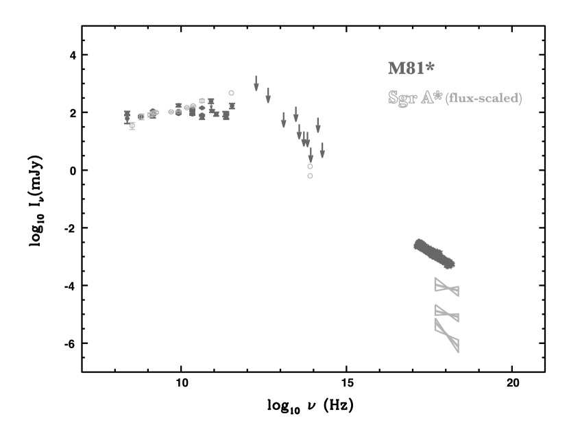
Figure 13: Comparison between total combined broadband spectrum of M81* (as in Fig. 19) and Sgr A*, where the data for Sgr A* have been scaled downwards by roughly an order of magnitude so the VLA-band fluxes are the same. The radio through NIR data for Sgr A* are the result of a simultaneous campaign presented in An et al. (2005). The X-ray “bowties” represent the quiescent, average daily Chandra flare and highest Chandra flare detected, respectively Baganoff et al. (2001); Baganoff (2003); Baganoff et al. (2003).

Our new simultaneous data reinforce the similarities previously reported between M81* and Sgr A*. In Fig. 13 we show the total M81* campaign spectrum, including the non-simultaneous IR/O/UV data upper limits discussed in §2.2, and overplot the simultaneous Sgr A* spectrum from An et al. (2005) along with the various Chandra X-ray spectra (Baganoff et al. 2001; Baganoff 2003; Baganoff et al. 2003). The Sgr A* data have been scaled downward by a factor of $\approx 10$ in order to ease visual comparison.

M81* and Sgr A* show remarkable similarities in the radio frequencies. Even though for M81*, within the GMRT error bars, we see no direct evidence for the free-free absorption turnover observed in Sgr A*, the slightly inverted spectra in both sources are still classic indicators of synchrotron self-absorption effects in the jet core emission. The M81* radio spectrum lies below that of Sgr A* at higher frequencies, and thus is less inverted than that of Sgr A*. This is expected for M81* in the context of self-absorbed, accelerating jet models as its lower inclination angle compared to Sgr A* would result in a less inverted spectrum. The jets in Sgr A* are presumed to be at a high inclination angle with respect to our line of sight (see the supporting evidence from the models presented by Markoff et al. 2007; Meyer et al. 2007). The spectra for M81* and Sgr A* both seem to peak near the submm range and then subsequently drop off towards the IR. Both sources also are consistent with sharing the same radio-IR power-law slope, if the M81* IR upper-limits are indicative of the underlying intrinsic spectrum. M81* and Sgr A*, however, clearly diverge from one another in the X-ray regime. On a relative scale, the M81* X-ray spectrum always lies above that for Sgr A*, with the latter source in its rare, bright flare states still falling short of the X-ray/radio flux ratio of M81*.

If M81* indeed has a “submm bump” as in Sgr A*, this would be only the second source where such a feature is observed. In Sgr A* this component has been associated alternatively with the base of a compact jet (Falcke & Markoff 2000; Markoff et al. 2001b), the regions of the accretion flow closest to the black hole (Narayan et al. 1998; Yuan et al. 2003), or with an inner Keplerian disk (Liu & Melia 2001). Regardless of the exact geometry, in Sgr A* this component now has been definitively associated with X-ray flares (Eckart et al. 2004, 2006b), and thus is of significant interest for understanding high-energy processes within tens of $r_{g}$ of the Sgr A* black hole. For the LLAGN class as a whole, it is important to understand if the flaring and coupling of the submm bump/X-ray emission in Sgr A* is typical. The X-rays in M81* have yet to show any flares of significant amplitude, while we have some evidence of variability in the submm. Thus in contrast to Sgr A*, the X-ray emission in M81* may not be due to the same physical component that yields the variable submm. As further described below, this has implications for the theoretical modeling of M81*.

These results for the submm band in particular are still tentative; more monitoring of this band as well as the millimeter range will determine whether an intrinsic submm bump is indicated. Massive amounts of dust are present in the region observed in these bands and could be contributing some level of flux. On the other hand, subsequent brief observations at 345 GHz using the SMA in 2005 (A. Peck, priv. comm.) show significant variability, yielding a flux density ranging from 300 mJy to 900 mJy over a period of 3 months from April to June 2006, consistent with the measurements made at the SMA in Feb 2005. These values are accurate to within about 20%, and thus the variability is clearly significant. These further data also support a rise in flux above the millimeter band. It is possible that the submm bump is a completely transient feature associated with flaring/ejecta, as has been suggested for Sgr A*. Confirming this strong variability as well as a detection of linear polarization would place stringent limits on any dust contribution, as well as the spectrum. With the advent of polarimetry at 345 GHz this year on the SMA, we have (with D. Marrone, PI) successfully proposed to search for linear polarization in M81*, which will hopefully resolve this issue in the near future.

5 Jet-dominated spectral models

5.1 Model description

One of the basic tenets of General Relativity is that black holes are essentially self-similar with regards to mass. An obvious possible consequence of this is a predictable scaling with mass of the accretion physics around black holes. If such a scaling exists, it would imply that the same underlying physical model could explain the continuum emission for stellar accreting black holes in XRBs as well as SMBHs. Likely complicating this simple picture are differences that could be introduced by accretion off one star compared to accretion off the winds of entire clusters of stars. Furthermore XRBs undergo state changes, which have yet to be clearly associated with the various AGN classes as would be naively expected if some of the AGN classes correspond to much longer lived state transitions.

So far the best case for such a mapping, referred to as the “fundamental plane of black hole accretion”, is the correspondence in characteristics between the sub-Eddington low/hard state of XRBs and LLAGN (Merloni et al. 2003; Falcke et al. 2004; Körding et al. 2006). The hard state of XRBs is characterized by weak accretion disk emission, and the presence of steady, compact jets (e.g. Fender 2006). These jets seem to increasingly dominate the power output of the system even as the total accretion rate decreases (Fender et al. 2003). Lending theoretical support to the idea of a fundamental plane, models of LLAGN as being dominated by outflows (e.g. Falcke & Markoff 2000; Markoff et al. 2001b; Yuan et al. 2002) also have been quite successful at explaining the broad continuum properties of hard state XRBs (e.g Markoff et al. 2001a, 2003). More recently, these outflow-dominated models have been refined further to account for strong geometrical constraints, for example, such as signatures of reflection off of cool material. The outflow models were developed to take advantage of data from recent simultaneous, multi-wavelength monitoring campaigns. Statistical fitting of the simultaneous broadband continua of several hard state XRBs, including finer features such as fluorescent Fe lines in their X-ray bands, have produced consistent trends among the physical parameters determined for this class of sources (Markoff et al. 2005; Migliari et al. 2007; Gallo et al. 2007, ; Maitra et al., in prep.).

In order to further test the principle of black hole accretion scaling with mass, and to enable a stronger physical comparison among M81*, Sgr A*, and their possible stellar-mass equivalents, we apply these same hard state XRB outflow-dominated models to the M81* spectra from our campaign. The only significant difference from the model application to XRBs is that the input mass for M81* is $\sim 10^{6}$ times larger. A more detailed description of this model can be found in the appendix of Markoff et al. (2005), and references therein; here we provide a brief summary.

The model was designed to test the premise that the magnetized, outflowing compact accretion disk coronae such as described in (e.g. Beloborodov 1999; Malzac et al. 2001; Merloni & Fabian 2002) can comprise the footpoints of collimated jets. Although magnetic fields are assumed to play a global role, the dynamics of the model do not include magnetic acceleration. There are two primary reasons for this choice. First, because the exact role of the fields in the dynamics is still under debate, including a magnetic pressure term explicitly would add more assumptions (and thus free parameters) to the model. Secondly, the observations suggest that the steady jets in the weakly accreting black hole state are less accelerated than the transient jets occurring near the Eddington limit (e.g. Fender 2006). The observations so far can thus be well-explained by a gas pressure dominated model. In addition, for M81* and Sgr A* in particular the inverted radio spectrum is also suggestive of adiabatic cooling in a jet with a broader opening angle ($\geq 20^{\circ}$), rather than a narrow jet as would be expected for magnetic collimation.

Aside from these points, there are four basic assumptions in the model: 1) the total power in the jets scales with the total accretion power at the innermost part of the accretion disk, $\dot{M}c^{2}$, 2) the jets are freely expanding and only weakly accelerated via their own internal pressure gradients, 3) the jets contain cold protons which carry most of the kinetic energy, while leptons dominate the radiation, and 4) some or all of the originally thermally distributed particles are accelerated into a power-law which is maintained along the rest of the jet via distributed acceleration.

The base of the jet consists of a small nozzle of constant radius where no bulk acceleration occurs. The nozzle absorbs our uncertainties about the exact nature of the relationship between the accretion flow and the jet, and fixes the initial value of most parameters. Beyond the nozzle, the jet expands laterally with its initial proper sound speed for a relativistic electron/proton plasma, $\gamma_{\rm s}\beta_{\rm s}c\sim 0.4c$. The plasma is weakly accelerated by the resulting longitudinal pressure gradient force, allowing an exact solution for the velocity profile via the Euler equation (see Falcke 1996). This results in a roughly logarithmic dependence of velocity upon distance from the nozzle, $z$. The velocity eventually saturates at large distances at Lorentz factors of $\Gamma_{\rm j}\gtrsim$2-3. The size of the base of the jet, $r_{0}$, is a free parameter and once fixed determines the radius as a function of distance along the jet, $r(z)$. There is no radial dependence in this model, and the opening angle is thus fixed by the velocity profile as a function of distance along the jets.

The model is most sensitive to the fitted parameter $N_{\rm j}$, which acts as a normalization. It dictates the power initially divided between the particles and magnetic field at the base of the jet, and is expressed in terms of a fraction of $L_{\rm Edd}$. Once $N_{\rm j}$ and $r_{0}$ are specified and conservation is assumed, the macroscopic physical parameters along the jet are determined. We assume that the jet power is roughly shared between the internal and external pressures. The radiating particles enter the base of the jet where the bulk velocities are lowest, with a quasi-thermal distribution of temperature $T_{e}$ (a fitted parameter). A significant fraction (here fixed at 75% based on results from the XRB fits mentioned above) of the particles are accelerated into a power-law tail at a location $z_{acc}$ (also a fitted parameter). The maximum energy the electrons can achieve is calculated explicitly by setting the local cooling and escape rates to the acceleration rate. Here we assume that the particles are accelerated via the most conservative case of diffusive shock acceleration with the magnetic field parallel to the shock normal (see Jokipii 1987). The acceleration rate depends on the plasma parameters $u_{\rm sh}$ and $\xi$, the relative velocity of the shock to the plasma in the shock frame, and the ratio between the mean free path for scattering and the gyroradius, respectively. These terms enter into the acceleration rate as $\epsilon_{\rm sc}\equiv\left(u_{\rm sh}/c\right)^{2}/\xi$. This is a free parameter in our fits, and since $\xi$ is thought to lie in the range $\sim 10$–$1000$, it provides a consistency check on the plasma velocities.

The particles in the jet radiatively cool via adiabatic expansion, synchrotron processes, and inverse Compton upscattering; however, adiabatic expansion is assumed to dominate the observed effects of cooling. While thermal photons from the accretion disk (via a multicolor blackbody model) are included as seed photons in the inverse Compton calculations, beaming reduces their energy density compared to the rest frame synchrotron photons (synchrotron self-Compton; SSC), except at the very base of the jet where they can be of the same order. The temperature $T_{\rm d}$ and total luminosity $L_{\rm d}$ of a thin accretion disk are also included as fitted parameters, but as this component is not an integral part of the outflow model, and not well constrained by this data set, we include these parameters mainly for a consistency check.

Aside from those mentioned above, the other main fitted parameters are the ratio of nozzle length to its radius, $h_{0}$, and the equipartition parameter between the magnetic field and the radiating (lepton) particle energy densities, $k$. Physical parameters such as the mass, inclination angle and distance are fixed at the observed values. Table 10 summarizes all the fitted jet parameters.

This model has provided a very good statistical description of the broadband radio through X-ray data from several XRBs. The data from this campaign observing M81* allows us to test the premise that sub-Eddington accretion in LLAGN can be described by the same physics as sub-Eddington accretion in low/hard state XRBs, even though the latter sources are over six orders of magnitude less massive than the former. This is the first time that our jet model has been applied to a “canonical” LLAGN, which thus allows for an interesting comparison to Sgr A*.

5.2 Fitting methodology

We explore two possible jet-model scenarios with our M81* data. The first scenario is an exact analog to the XRB fits, where the particles are presumed to enter the nozzle in a quasi-thermal distribution that is later accelerated in the jet. This scenario was also explored for Sgr A*, where we determined that the acceleration must be either extremely weak or lacking, or that it must occur extremely far out in the jets, in order to prevent the presence of a predicted power-law violating the observed IR flux values (Markoff et al. 2007). The second scenario assumes that the particles enter the jets in a full power-law distribution, as may occur if jet formation is associated with a shock in the inner regions of the accretion flow (Koide et al. 2000). This scenario was also explored for Sgr A*, where in order to be consistent with the quiescent spectrum the acceleration must be sufficiently weak to result in an electron particle distribution power-law no harder than $p\sim 3.8$ (Markoff et al. 2007).

In exploring these models, fits to the individual ObsIds for the Chandra data were simultaneously carried out over the 0.5–7 keV band for the MEG data and the 0.7–8 keV band for the HEG data. Each dataset was grouped to have a minimum signal-to-noise of 5 and a minimum of four wavelength channels per bin. Because there are hundreds of X-ray data points compared to the radio/submm data, we initially set the radio/submm data errors to $<1\%$ to “weight” the significance of the sparser lower-frequency data in the fitting procedure. But because the jet model produces a predominantly smooth radio spectrum (i.e., it does not account for the waves of variability likely moving through the radio spectrum), and because the radio error bars are for the most part small compared to the observation-to-observation variability, in our final joint radio/X-ray fits we add 20% error bars in quadrature to the statistical error bars for the radio data. In this manner we decrease the likelihood that the jet models fall into local minima, and ensure that they instead more fairly represent the average radio properties.

We also present a series of fits wherein we simultaneously consider the radio and X-ray data from the entire campaign. We again add 20% error bars in quadrature to the statistical error bars of the radio data. For the Chandra data we use the ISIS combine_datasets function to combine the HEG data into a single spectrum and to combine the MEG data into a single spectrum. For each of these spectra we further group the data such that there is a minimum of 100 counts and a minimum of 32 energy channels per bin.

The addition of 20% error bars to the radio and optical data acts to subsume both instrinsic variability, and allows for any systematic calibration differences among the different detectors. However, one might worry that the radio and optical data would then apply little statistical leverage on the fits. In fact, owing to the 2.5 to 9 orders of magnitude energy differences between the X-ray and UV/radio data, their effect far outweighs the simple contribution calculated to the overall $\chi^{2}$. For example, if one pivots a power-law with $\Delta\Gamma=0.01$ at 1 keV, the change in slope would yield well over a 20% difference in the radio regime (i.e., greater than our added error bars) while giving only a 2% difference at 8 keV (i.e., substantially less than the X-ray data bars). The jet models are thus predominantly constrained by the radio data via this effect, rather than their contribution to the $\chi^{2}$ statistic.

In order to illustrate this explicitly, in Fig. 14 we present the radio residuals for a fit performed solely in the X-ray regime, using jet model parameters somewhat different than the typical (based on fitting X-ray binaries) values discussed here. The model provides an extremely good fit to the X-ray data, with a change of $\Delta\chi^{2}=1.2$ compared to our best fit from the broadband spectrum. This model, however, fails completely in the optical and radio regime, even with our expanded radio error bars. Thus the simultaneous radio/submm data especially are crucial for excluding large regions of “reasonable” parameter space for the jet models. The X-ray data alone simply cannot constrain jet physics.

The resulting parameter differences between our canonical fits and the two fits utilizing non-simultaneous upper limits in the infra-red and optical, further emphasizes that broadening the multi-wavelength coverage is clearly very desirable. The jet model fits do present a number of “local minima”, which are also evidenced in the error bars for some parameter fits. Occasionally we find large parameter error bars– again an indication of inherent degeneracies in this complex theoretical model that we expect would be reduced with broader wavelength coverage. We also occasionally find parameter error bars that are unusually small. This is sometimes attributable to the fact that the radio data points do not represent a smoothed, averaged behavior, whereas the theoretical model does represent such an idealization to some extent. If a fit fortuitously passes almost exactly through a few radio points, the fits occasionally become very localized to that fit local minima. Such a local minimum might be slightly removed from a separate local minimum associated with a different subset of the radio points. The added 20% radio error bars tends to reduce, but not entirely eliminate, this behavior of the fits. Ultimately a time-dependent model is required to completely account for these effects.

For the X-ray band specifically, Young et al. (2007) fit a series of emission and absorption lines to the combined M81* Chandra spectra. To account for the presence of these features in the spectra, for all of our fits we added the complete set of lines from Young et al. (2007), but with there wavelengths frozen to those found in that work, and their widths frozen to $10^{-4}$ eV. Only the line amplitudes were allowed to vary in the fits.

5.3 Results and interpretation

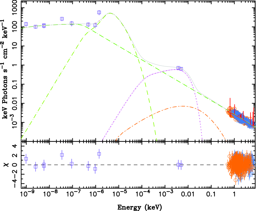
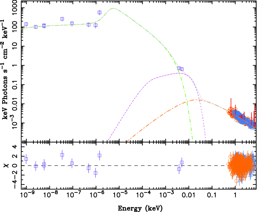
Figure 15: Model fit to broadband February data with residuals. Left: Fit with initially Maxwellian leptonic distribution, Right: leptonic power-law distribution fit. The symbols represent the data, while the solid red line is the model fit in detector space. The other components are not convolved with the detector matrices and serve only to indicate the contributing components to the continuum model. Solid (grey): total spectrum, Dot-longdashed (light green): pre-acceleration inner jet synchrotron emission, Dot-longdashed (darker green): post-acceleration outer jet synchrotron, Dot-longdash-shortdash (orange): Compton emission from the inner jet (including external disk photons as well as synchrotron self-Compton), Dots-shortdash (magenta): thermal multicolor-blackbody disk model.

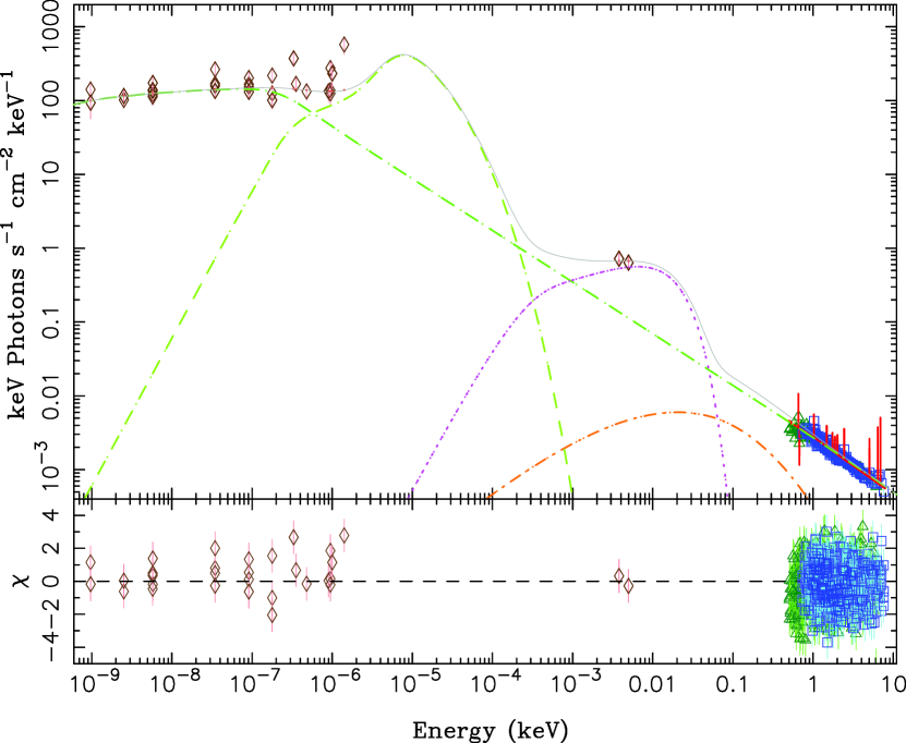
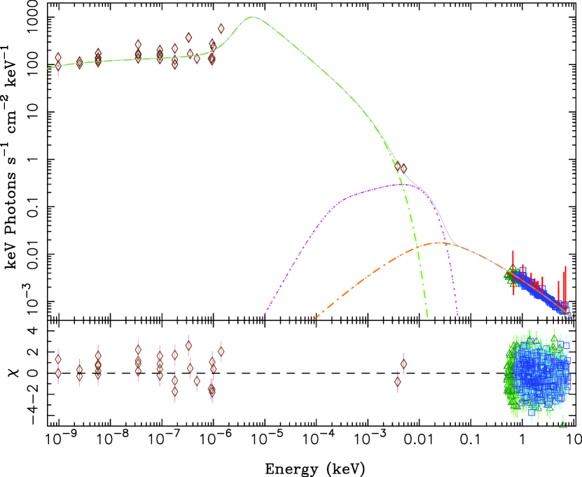
Figure 17: Model fit to combined set of all broadband observations, with the same symbol/line definitions as Fig. 15.

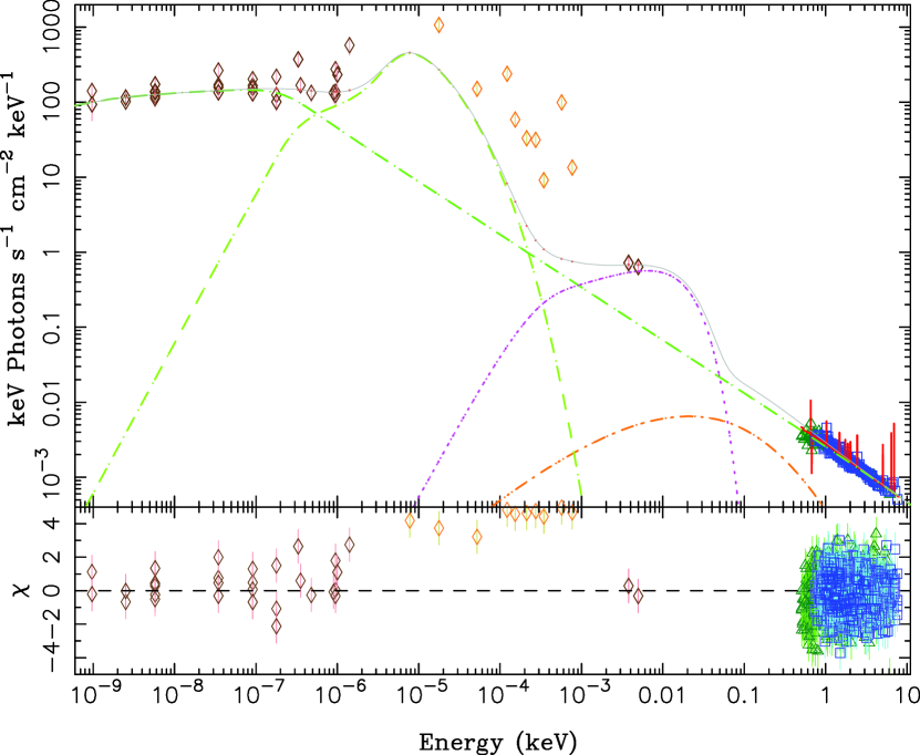
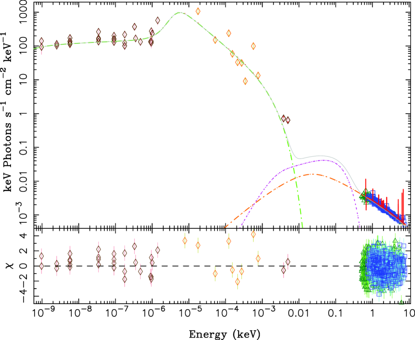
Figure 19: Model fit to combined set of all broadband observations, with the addition of several nonsimultaneous upper limits taken from the literature from HST, Spitzer, ISO and MIRLIN (Grossan et al. 2001; Gordon et al. 2004; Murphy et al. 2006) included as data points with 20% systematic errors. Same symbol/line definitions as Fig. 15.

Figs. 15 & 16 present our best fits of each type of model to the most comprehensive single observation in February, while Figures 17 & 18 show the fits to all campaign data combined. Non-simultaneous data points from HST (Maoz et al. 2005) have, however, been included with error bars increased to 20% in order to guide the fits in the observational gap that otherwise extends over six decades of photon frequency. Figs. 19 & 20 present additional fits which also include the upper limits from the simultaneous Lick Observatory observations, as well as several non-simultaneous detections taken from the literature (but here used as upper limits since they likely include non-nuclear emission) for ISO, MIRLIN, HST and Spitzer (Grossan et al. 2001; Gordon et al. 2004; Murphy et al. 2006). All of these upper limit data were treated as measured points at their upper values, with additional 20% error bars applied. Given the similarity in the shape of the submm through optical/UV data from M81* compared to what is seen in Sgr A* and NGC 4258, it seemed worthwhile investigating scenarios that included these limits as estimates of the true, underlying spectra.

The values for the fitted parameters with 90% confidence errors for all fits, including the individual data set fits not shown here, are presented in Tables  11– 14.

It is clear that the model provides a very good description of the individual observations, and to a lesser extent the combined data set. The latter data set obviously includes variations, especially for the non-X-ray data, for which the steady-state model cannot account. What is most striking about these fits is that the overall values for the fitted parameters fall into remarkably similar ranges compared to the parameter values for hard-state XRBs and Sgr A*.

We first consider the model with an initial power-law electron distribution. The power-law electron distribution has previously been applied to spectra from Sgr A*, but not to any XRB spectra. Compared to the the range of Sgr A* fits explored in Markoff et al. (2007), the fits to the M81* spectra a similarly find a very compact jet base and an electron temperature of $\approx 10^{11}$ K. There are, however, significant differences which are likely influenced by the lower X-ray/radio flux ratio in Sgr A*, as well as the fact that Sgr A*, as a fraction of Eddington luminosity, is over four orders of magnitude lower compared to M81*. Whereas M81* shows indications of a weak accretion disk, no such component has been observed in Sgr A*. Whether assumed to occur near the base, as for the power-law (PL) fits, or further out in the jets, as in the Maxwellian (MXW) fits, the M81* spectra prefer solutions with more efficient particle acceleration. That is, the electron power-law index $p=2.4$–2.8, whereas for Sgr A* $p$ is always $>3$. The M81* particle distribution also shows more cooling than in Sgr A*, as indicated by the $\sim 10$ times smaller $\gamma_{\rm max}$ in M81*. These differences go far to explain why the weak jets of M81* have been easier to discern than those in Sgr A*. Beyond the fact that we are not viewing M81* through the Galactic plane scattering screen, more particle acceleration leads to more optically thin jet emission, which in turn increases the size of the photosphere at a given frequency. Thus M81*’s jets, with radiating particles accelerated into a canonical power-law, would be predicted to have a much larger photosphere at the same frequency than Sgr A*’s.

The equipartition parameter, $k$, in M81* is very similar to the values found in XRBs, favoring mild magnetic domination of the internal energy. Sgr A* on the other hand seems to be the only source we have studied so far which favors a stronger magnetic energy density ($k\sim 15$), bucking the trend seen here in M81* and in XRBs for a correlation between total jet power and equipartition parameter. Because we have no information about the non-thermal X-ray spectrum of Sgr A* in quiescence, however, this parameter may not be well constrained, but it is something to keep in mind for future explorations.

The fitted jet nozzle scale height in M81* is not well-constrained by these fits. However, the fits that include upper limits as estimates of the IR through optical spectra clearly select out a more elongated base/corona. Thus to strongly constrain the value of the nozzle scale height, further simultaneous millimeter through IR/optical observations are necessary.

Looking at the Maxwellian model fits, which have been applied to both Sgr A* and hard state XRBs, we see the same trends when comparing to the Sgr A* fits. For the MXW cases, we can also compare acceleration efficiency by the need for a power-law tail in the best-fit electron spectrum. Both M81* and XRBs are consistent with a high rate, here frozen to 75%, as compared to Sgr A* where only a small fraction of particles are accelerated. In Sgr A*, the contribution of the tail also is minimized by acceleration occurring at quite large distances from the jet base. In contrast, the acceleration in M81* occurs at the same location as seen in XRBs ($\sim 10-100\,r_{g}$). In fact, even though we are probing a fairly low fractional Eddington luminosity compared to the previously fit XRBs, nearly all fitted parameters for the MXW fits to M81* fall into the exact same ranges as those seen in hard state XRBs. The only major parameter difference is the electron temperature, which is a factor of $\sim 2-3$ lower in XRBs. These results thus provide very strong support for the mass-scaling of accretion physics, at least for weakly accreting black holes.

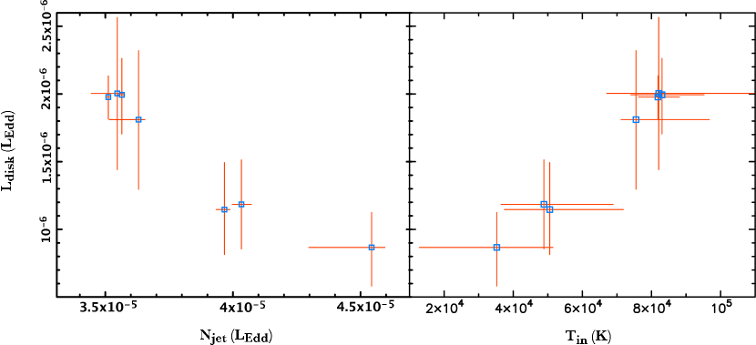
Figure 21: Possible correlations between the total accretion disk luminosity and the jet normalization and inner disk temperature, based on the Maxwellian model fits to separate and combined data sets described in Figs. 15–20 and Tables 13–14.

By comparing the fits to individual data sets, we can look for meaningful correlations in the parameters on timescales impossible to probe in XRBs, as weeks to months in M81* would correspond roughly to sub-second variations in a typical XRB. Overall there are more obvious correlations among the MXW fit parameters than compared to the PL fit parameters. This fact leads us to consider the MXW fits as more likely probing more real physical effects. However, simultaneous constraints in the IR through UV are necessary to conclusively break this degeneracy. A selection of the strongest correlations are shown in Figs. 21 & 22.

Given the lack of simultaneous constraints on the IR through UV range, it is somewhat surprising to see some trends linking intrinsic jet parameters to the accretion disk parameters. There is a clear anti-correlation between the disk flux and the energy input to the jet. This may in fact be similar to the observed anti-correlation between soft and hard X-ray fluxes seen in hard state XRBs, such as Cyg X-1 (see Wilms et al. 2006). For M81*, the higher disk flux is driven by an increase in the fitted disk temperature, but given that we do not have simultaneous data directly in the spectral region where the disk spectrum is most prominent (see Fig. 14), we cannot in fact be sure that the correlation is not systematic.

More interesting are the correlations detected between the equipartition parameter $k$ and other fitted parameters. Along with the total normalized power $N_{\rm jet}$, $k$ seems to be one of the most important parameters for the jet model. Because it dictates the distribution of energy between the radiating particles and the magnetic fields, it effects the synchrotron/inverse Compton ratio, and can in some sense compensate for losses in the particle energy density due to, for instance, temperature decreases. As the temperature goes down, more energy is needed is needed in the magnetic energy to maintain the same synchrotron emission, thus requiring an increase in $k$. Similarly, a wider jet base results in a lower particle number density and thus $k$ must again be increased to maintain the same radiative fluxes. The most interesting correlation, however, is that between the jet power and the equipartition. We seem to be seeing a trend towards stronger magnetic powers relative to the radiating particles with increasing total jet power. With the exception of Sgr A* (but see above for a reason to possibly discount this source in this regard), this trend is also seen in individual fits to hard state XRBs (Markoff et al. 2005; Migliari et al. 2007; Gallo et al. 2007, ; Maitra et al. in prep.). One possible interpretation of this is that the magnetic fields are more efficiently generated at higher accretion rates. After increasingly building up, an explosive release of this energy at some critical accretion rate may be responsible for driving the transient, and much more relativistic, ejecta seen in transition to the XRB hard state.

6 Conclusions

Our simultaneous broadband campaign on the LLAGN M81* has generated five individual spectra, spread over 6 months, as well as a combined spectrum, that can be readily compared to other LLAGN, such as Sgr A*, as well as hard-state, weakly accreting X-ray binaries. These data definitively confirm for the first time many species of line emission from the accretion flow of an LLAGN (Young et al. 2007), and we have confirmed previous detections of variability across the entire spectrum. The radio through submm in particular shows significant levels of both intraday and longer term variability. We also see indications for adiabatically decaying “flares” moving out along the jets.

The simultaneous, broadband nature of these data has allowed us to fit the spectra with an outflow-dominated model developed for hard state XRBs, that also has been used to understand our extremely subluminous Galactic nucleus, Sgr A*. We find several interesting results based on these spectral fits. Compared to Sgr A*, M81* is not only much more luminous, but also more of its accretion energy is funneled into accelerating and maintaining power-law distributions of the radiating particles. Otherwise, the geometry and particle thermal/minimum temperatures seem to be very consistent between these two sources. We are currently conducting a campaign of similar scope for the LLAGN NGC 4258 (Nowak et al., Reynolds et al., in prep.), which will provide a third object to this “sample” of extensive, simultaneous multi-wavelength datasets for LLAGN.

The most remarkable result of our modeling is the discovery that M81* seems to behave just like a hard state XRB, despite it being over six orders of magnitude more massive, and accreting at a fractional Eddington luminosity somewhat lower than for the jet model fits to XRBs. The best fit parameters all fall into the same range as those found for XRBs, with the exception of the particle initial temperature/minimum energy, and the nozzle length. We do not consider the latter significant, however, since it cannot be well constrained by this data set. The temperature difference, on the other hand, could be more notable since it is shared with fits from other LLAGN (Markoff et al. 2001b; Yuan et al. 2002). If particles in LLAGN enter the jets with a factor of 2–3 higher temperature than XRBs, this could be due to the lower cooling rates for the comparatively less compact LLAGN jets given the same power and size in mass-scaling units of $L_{\rm Edd}$ and $r_{g}$. Our results provide an independent confirmation of the mass-scaling accretion physics suggested by the fundamental plane of black hole accretion described in § 5.

Finally, given the $>20\%$ variations seen in the radio within the campaign, as well as in comparison with prior observations, and the factor of $\sim 5$ times smaller average X-ray flux, it is clear that the differences between average/non-simultaneous measurements and simultaneous multiwavelength observations may be quite important for LLAGN, and perhaps AGN as well. In particular these variations becomes relevant for the fundamental plane of black hole accretion. Sub-Eddington accreting black holes show a correlation with slope $\approx 0.6$–0.7 between the logarithms of the radio and X-ray luminosities, with an effective mass-dependent normalization. The exact values of the coefficients are important for placing stringent limits on the processes responsible for the emission. To date, the coefficients primarily have been determined from samples of AGN/LLAGN with non-simultaneous or averaged values for the radio and X-ray luminosities. Given the now confirmed significant broadband variability of M81*, taking average values will likely lead to incorrect determinations for the correlation coefficients. To quantify this possibility, we use the quasi-simultaneously measured radio and X-ray luminosities from this campaign and redo the fundamental plane statistical analysis of Markoff (2005). We find a difference of 8% in the radio/X-ray correlation slope, and a difference of 50% in the mass-dependence coefficient! Our results therefore strongly argue for some level of care in conclusions based on non-(quasi)simultaneous observations.

Table 1: Log of 2005 February 23–25 Observations

Instrument	Energy/$\nu$	Start Time (UT)	End Time (UT)
GMRT	235/610 MHz	23 Feb 14:15	23 Feb 22:57
GMRT	1390 MHz	24 Feb 13:56	24 Feb 16:23
VLA	1.4/8.4/22/43 GHz	24 Feb 05:00	24 Feb 12:30
PdBI	115/230 GHz	24 Feb 01:11	24 Feb 19:45
SMA	345 GHz	24 Feb 04:44	24 Feb 17:20
Lick	K/J/H band	24 Feb 08:13	24 Feb 11:40
Lick	H band	25 Feb 09:28	25 Feb 09:49
Chandra HETGS	0.5–8 keV	24 Feb 06:56	24 Feb 20:50

Note. — In this and Tables 2–4, the observing times represent the beginning and end of dedicated observational time. Integrated time is less than the full period, as calibration was performed intermittently during the intervals. The Chandra ObsId for this observation was 6174.

Table 2: Log of 2005 July 12–16 Observations

Instrument	Energy/$\nu$	Start Time (UT)	End Time (UT)
GMRT	235/610 MHz	12 Jul 06:31	12 Jul 13:16
GMRT	1390 MHz	15 Jul 04:05	15 Jul 08:11
VLA	1.4/8.4/22/43 GHz	13 Jul 04:56	13 Jul 23:00
VLBA	8.4 GHz	13 Jul 17:30	14 Jul 05:30
PdBI	80.5/241.4 GHz	14 Jul 06:50	15 Jul 13:50
SMA	230 GHz	15 Jul 21:25	16 Jul 04:38
Chandra HETGS	0.5–8 keV	14 Jul 01:44	14 Jul 17:28
Chandra HETGS	0.5–8 keV	14 Jul 19:25	15 Jul 13:20

Note. — VLBA imaging at 22 GHz and SMA imaging at 230 GHz both failed due to poor weather. The Chandra ObsId for this observation were 6346 and 6347.

Table 3: Log of 2005 July 18–20 Observations

Instrument	Energy/$\nu$	Start Time (UT)	End Time (UT)
VLA	1.4/8.4/22/43 GHz	19 Jul 16:44	19 Jul 23:07
PdBI	86.2/218.2 GHz	19 Jul 23:17	20 Jul 16:07
SMA	230 GHz	18 Jul 21:25	19 Jul 03:25
Chandra HETGS	0.5–8 keV	19 Jul 14:25	20 Jul 15:25

Note. — The Chandra ObsId for this observation was 5601.

Table 4: Log of 2005 August 14–15 Observations

Instrument	Energy/$\nu$	Start Time (UT)	End Time (UT)
VLA	1.4/8.4/22/43 GHz	14 Aug 13:19	14 Aug 19:15
SMA	230 GHz	14 Aug 19:37	15 Aug 01:30
Chandra HETGS	0.5–8 keV	14 Aug 09:50	14 Aug 20:57

Note. — PdBI experienced bad weather and no data were taken. The Chandra ObsId for this observation was 5600.

Table 5: Results of the GMRT Observations

Date of	Frequency	No. of good	% of good	Resoln.	Flux density	rms
Observn	MHz	Antennae	Data	′′	mJy	mJy
2005 Feb 24	1390	27	75	5x3	$80.1\pm 2.1$	0.24
2005 Jul 15	1390	26	80	5x3	$114.8\pm 1.1$	0.32
2005 Feb 23	610	27	80	8x7	$67.4\pm 1.3$	0.45
2005 Jul 12	610	29	90	8x6	$76.3\pm 1.2$	0.42
2005 Jul 26	610	27	75	9x5	$72.4\pm 3.1$	0.49
2005 Feb 23	235	30	55	18x13	$93.5\pm 14.9$	4.95
2005 Jul 12	235	28	70	19x12	$61.8\pm 20.9$	3.80

Table 6: Comparison of calibration observations of SN 1993J for GMRT and VLA

Date	Instrument	Frequency (GHz)	Flux density (mJy)
2005 Jul 14	VLA	1.4	$9.64\pm 0.56$
2005 Jul 14	VLA	8.4	$2.43\pm 0.29$
2005 Jul 15	GMRT	1.4	$9.00\pm 0.52$
2005 Aug 14	VLA	1.4	$10.23\pm 0.80$
2005 Aug 14	VLA	8.4	$1.87\pm 0.20$

Table 7: Results of the VLA Observations

Date of	Frequency	Flux density	rms
Observn	GHz	mJy	mJy
2005 Feb 24	43	–	–
2005 Jul 13	43	$66.5\pm 8.5$
2005 Jul 19	43	$143.4\pm 3.1$
2005 Aug 14	43	$82.1\pm 2.4$
2005 Feb 24	22	$101\pm 20$
2005 Jul 13	22	$86.4\pm 5.8$
2005 Jul 19	22	$133.6\pm 0.6$
2005 Aug 14	22	$109.6\pm 1.4$
2005 Feb 24	8.4	$176\pm 20$
2005 Jul 13	8.4	$89.7\pm 2.6$
2005 Jul 19	8.4	$105.1\pm 0.4$
2005 Aug 14	8.4	$112.5\pm 0.1$
2005 Feb 24	1.4	$75\pm 10$
2005 Jul 13	1.4	$91.9\pm 0.3$
2005 Jul 19	1.4	$92.6\pm 0.9$
2005 Aug 14	1.4	$89.5\pm 0.6$

Note. — Due to bad weather, no data were taken at 43 GHz in February.

Table 8: Results of the PdBI observations

Date of	Frequency	No. of good	% of good	Flux density	rms
Observn	GHz	Antennae	Data	mJy	mJy
2005 Feb 24	115.3	6	90%	$88.0\pm 11.7$	–
2005 Jul 14	80.5	5	50%	$241.2\pm 33.8$
2005 Jul 19	86.2	5	98%	$118.7\pm 11.4$
2005 Feb 24	230.5	6	90%	$85.6\pm 17.8$
2005 Jul 14	241.4	5	30%	$181.2\pm 39.1$
2005 Jul 19	218.2	5	90%	$74.8\pm 13.3$

Note. — The listed flux densities result from the mean and standard deviation of the lightcurves obtained during the observations (Schödel et al. 2007).

Table 9: Results of the SMA Observations

Date of	Frequency	No. of	Flux density
Observn	GHz	Antennae	mJy
2005 Feb 24	340.7	7	$378.7\pm 70.0$
2005 Jul 18	225.4	7	$182.8\pm 36.0$
2005 Aug 14	225.4	7	$91.5\pm 15.3$

Table 10: Summary of jet model parameters

Parameter	Meaning
Both models
$N_{\rm jet}$	Jet normalized power
$r_{0}$	Size of jet base
$T_{e}$	Temperature of particles entering base of jet
$p$	Energy index of electron power-law tail ($N_{e}\propto E_{e}^{-p}$)
$k$	Equipartition parameter: the ratio of energy density in the magnetic field
	to energy density in the radiating particles
$h_{\rm ratio}$	Ratio of jet nozzle length to nozzle radius
$L_{\rm d}$	Accretion disk bolometric luminosity
$T_{d}$	Innermost accretion disk temperature
Powerlaw (PL) model
$\gamma_{\rm max}$	Maximum Lorentz factor of electron distribution
Maxwellian (MXW) model
$z_{\rm acc}$	Location at which particles are first accelerated to produce powerlaw tail
$\epsilon_{\rm sc}$	Particle acceleration efficiency parameter; $\epsilon_{\rm sc}\equiv(u_{\rm sh}/c)^{2}/\xi$ where $u_{\rm sh}$ is the relative
	velocity of the shock to the plasma in the shock frame, and $\xi$ is the
	ratio between the mean free path to the gyroradius.

Table 11: Jet Model Fits to M81^∗ (PL)

Obs ID	Ljet	$r_{0}$	$T_{e}$	$p$	$k$
	($10^{-5}$ LEdd)	($GM/c^{2}$)	($10^{10}$ K)
6174	$4.207^{+0.013}_{-0.019}$	$4.536^{+0.028}_{-0.000}$	$10.00^{+0.02}_{-0.03}$	$2.729^{+0.003}_{-0.003}$	$1.019^{+0.010}_{-0.015}$
6346	$4.318^{+0.020}_{-0.019}$	$4.655^{+0.016}_{-0.075}$	$10.07^{+0.03}_{-0.03}$	$2.797^{+0.003}_{-0.171}$	$1.222^{+0.018}_{-0.017}$
6347	$4.316^{+0.019}_{-0.016}$	$4.657^{+0.013}_{-0.078}$	$10.06^{+0.03}_{-0.03}$	$2.798^{+0.002}_{-0.005}$	$1.217^{+0.017}_{-0.016}$
5601	$4.295^{+0.016}_{-0.015}$	$5.190^{+0.015}_{-0.002}$	$9.90^{+0.02}_{-0.02}$	$2.798^{+0.002}_{-0.202}$	$1.471^{+0.017}_{-0.016}$
5600	$4.357^{+0.027}_{-0.026}$	$4.936^{+0.019}_{-0.001}$	$9.89^{+0.04}_{-0.04}$	$2.628^{+0.007}_{-0.006}$	$1.075^{+0.021}_{-0.020}$
ALL	$4.238^{+0.009}_{-0.004}$	$4.553^{+0.003}_{-0.000}$	$10.55^{+0.01}_{-0.01}$	$2.800^{+0.028}_{-0.002}$	$1.028^{+0.005}_{-0.004}$
ALL	$4.211^{+0.012(+0.146)}_{-0.007(-0.003)}$	$4.553^{+0.005(+0.637)}_{-0.009(-0.017)}$	$10.56^{+0.02(-0.48)}_{-0.01(-0.66)}$	$2.800^{+0.000(-0.001)}_{-0.003(-0.172)}$	$1.029^{+0.009(+0.442)}_{-0.004(-0.009)}$

Note. —

Table 12: Jet Model Fits to M81^∗ (PL), continued

Obs ID	$h_{ratio}$	$\Gamma$	Ld	$T_{\rm d}$	$\chi^{2}$/DoF	$\chi^{2}_{\rm red}$
			($10^{-7}$ LEdd)	($10^{5}$ K)
6174	$10.702^{+1.625}_{-0.018}$	$34.68^{+1.19}_{-0.46}$	$7.9^{+1.9}_{-1.9}$	$0.48^{+0.18}_{-0.10}$	504.3/472	1.07
6346	$12.949^{+0.021}_{-0.032}$	$26.46^{+1.17}_{-0.97}$	$13.0^{+3.4}_{-3.4}$	$0.50^{+0.19}_{-0.11}$	529.4/536	0.99
6347	$12.945^{+0.020}_{-0.030}$	$27.92^{+1.29}_{-0.96}$	$12.9^{+3.7}_{-3.4}$	$0.53^{+0.19}_{-0.12}$	627.2/605	1.04
5601	$11.782^{+1.961}_{-0.006}$	$30.25^{+1.24}_{-1.00}$	$26.5^{+8.1}_{-8.0}$	$1.11^{+0.39}_{-0.21}$	818.4/782	1.05
5600	$9.836^{+1.942}_{-0.098}$	$21.12^{+0.75}_{-0.74}$	$13.9^{+3.3}_{-3.3}$	$0.49^{+0.16}_{-0.11}$	380.4/321	1.19
ALL	$10.663^{+1.241}_{-0.000}$	$32.34^{+0.14}_{-1.39}$	$10.6^{+1.8}_{-1.8}$	$0.60^{+0.13}_{-0.07}$	574.0/292	1.97
ALL	$11.412^{+1.168(+1.538)}_{-0.749(-1.575)}$	$35.07^{+0.58(-0.40)}_{-1.05(-13.95)}$	$7.4^{+1.9(+19.1)}_{-1.6(+0.6)}$	$0.59^{+0.17(+0.52)}_{-0.11(-0.11)}$	422.7/282	1.50

Note. —

Table 13: Jet Model Fits to M81^∗ (MXSW)

Obs ID	Ljet	$r_{0}$	$T_{e}$	$p$	$k$	$z_{acc}$
	($10^{-5}$ LEdd)	($GM/c^{2}$)	($10^{10}$ K)			($GM/c^{2}$)
6174	$4.543^{+0.052}_{-0.164}$	$4.63^{+0.52}_{-1.61}$	$8.45^{+0.13}_{-0.51}$	$2.424^{+0.024}_{-0.002}$	$1.842^{+0.061}_{-0.115}$	$142.0^{+14.0}_{-19.3}$
6346	$3.630^{+0.025}_{-0.114}$	$1.78^{+0.25}_{-0.24}$	$11.49^{+0.11}_{-0.26}$	$2.407^{+0.012}_{-0.002}$	$1.304^{+0.022}_{-0.338}$	$131.6^{+33.4}_{-9.6}$
6347	$3.547^{+0.022}_{-0.102}$	$1.96^{+0.26}_{-0.04}$	$11.47^{+0.07}_{-0.08}$	$2.413^{+0.002}_{-0.001}$	$1.298^{+0.019}_{-0.073}$	$124.4^{+6.3}_{-2.5}$
5601	$3.967^{+0.021}_{-0.032}$	$3.13^{+0.07}_{-0.09}$	$10.14^{+0.06}_{-0.07}$	$2.401^{+0.001}_{-0.001}$	$1.503^{+0.019}_{-0.038}$	$192.2^{+0.8}_{-38.7}$
5600	$4.033^{+0.039}_{-0.036}$	$2.88^{+0.14}_{-0.38}$	$10.13^{+0.09}_{-0.10}$	$2.403^{+0.002}_{-0.002}$	$1.490^{+0.032}_{-0.027}$	$193.5^{+49.8}_{-0.3}$
ALL	$3.512^{+0.007}_{-0.009}$	$2.42^{+0.04}_{-0.05}$	$11.60^{+0.02}_{-0.02}$	$2.412^{+0.002}_{-0.001}$	$1.376^{+0.006}_{-0.502}$	$143.9^{+0.1}_{-22.0}$
ALL	$3.565^{+0.011(+0.979)}_{-0.015(-0.018)}$	$2.40^{+0.06(+2.23)}_{-0.08(-0.61)}$	$11.41^{+0.04(+0.08)}_{-0.07(-2.96)}$	$2.409^{+0.001(+0.015)}_{-0.001(-0.008)}$	$1.340^{+0.010(+0.502)}_{-0.026(-0.042)}$	$144.4^{+1.5(+49.1)}_{-22.5(-20.0)}$

Note. —

Table 14: Jet Model Fits to M81^∗ (MXSW), continued

Obs ID	$h_{ratio}$	$f_{sc}$	Ld	$T_{\rm d}$	$\chi^{2}$/DoF	$\chi^{2}_{\rm red}$
			($10^{-7}$ LEdd)	($10^{5}$ K)
6174	$10.490^{+0.622}_{-3.861}$	$245.8^{+47.9}_{-21.3}$	$8.7^{+2.6}_{-2.9}$	$0.35^{+0.16}_{-0.22}$	497.0/471	1.06
6346	$5.224^{+0.148}_{-0.896}$	$516.2^{+59.8}_{-43.8}$	$18.1^{+5.1}_{-5.1}$	$0.76^{+0.21}_{-0.04}$	533.8/535	1.00
6347	$7.432^{+0.279}_{-1.152}$	$63.1^{+7.7}_{-4.8}$	$20.0^{+5.6}_{-5.6}$	$0.82^{+0.27}_{-0.15}$	608.4/604	1.01
5601	$15.090^{+0.278}_{-0.860}$	$157.8^{+15.7}_{-12.9}$	$11.5^{+3.5}_{-3.3}$	$0.51^{+0.21}_{-0.13}$	826.0/781	1.06
5600	$11.436^{+1.757}_{-0.813}$	$92.8^{+17.9}_{-15.7}$	$11.8^{+3.3}_{-3.3}$	$0.49^{+0.20}_{-0.12}$	322.8/320	1.01
ALL	$7.799^{+0.063}_{-0.020}$	$206.1^{+1.1}_{-0.1}$	$19.8^{+1.6}_{-1.6}$	$0.82^{+0.06}_{-0.06}$	576.1/291	1.98
ALL	$7.586^{+0.179(+7.504)}_{-0.191(-2.361)}$	$206.2^{+0.6(+310.0)}_{-0.8(-143.1)}$	$19.9^{+2.7(+0.1)}_{-2.9(-11.3)}$	$0.83^{+0.12(-0.01)}_{-0.09(-0.48)}$	379.4/281	1.35

Note. —

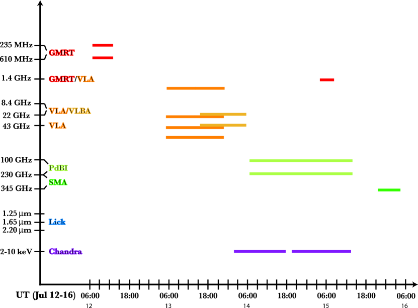
Figure 3: Schematic overview of the 2005 July 12-16 period. Exact times are shown in Table 2.

Figure 4: Resolved core-jet structure from the 8.4 GHz VLBA+Effelsberg observations.The synthesized beam of 0.6 mas is shown in the lower left hand corner. Contours are 0.5, 1, 2, 4, 8, 16, 32, and 64 mJy.

Figure 12: Comparison of 1mm PdBI and SMA observations in July and August.

Figure 14: As an illustration of the importance of broadband data for constraining jet models, we show here the radio data residuals for a fit to the X-ray data alone for Chandra ObsID 5600 (14 Aug). Top panel: ratio of data to model. Bottom panel: Change in $\chi^{2}$ compared to the best fit presented below, where 20% systematic error bars again have been added in quadrature to the radio data error bars. This fit results in jet parameters $z_{acc}\approx 1100$ and $h_{ratio}\approx 1.7$, ${\rm L_{jet}}$ and $r_{\rm 0}$ are at twice the typical values found in the fits presented in the tables, and $T_{e}$ is at one third the typical value presented in the tables. This fit is almost indistinguishable from the tabulated fits in the X-ray regime ($\Delta\chi^{2}=1.2$), but fails completely in the optical and radio regime.

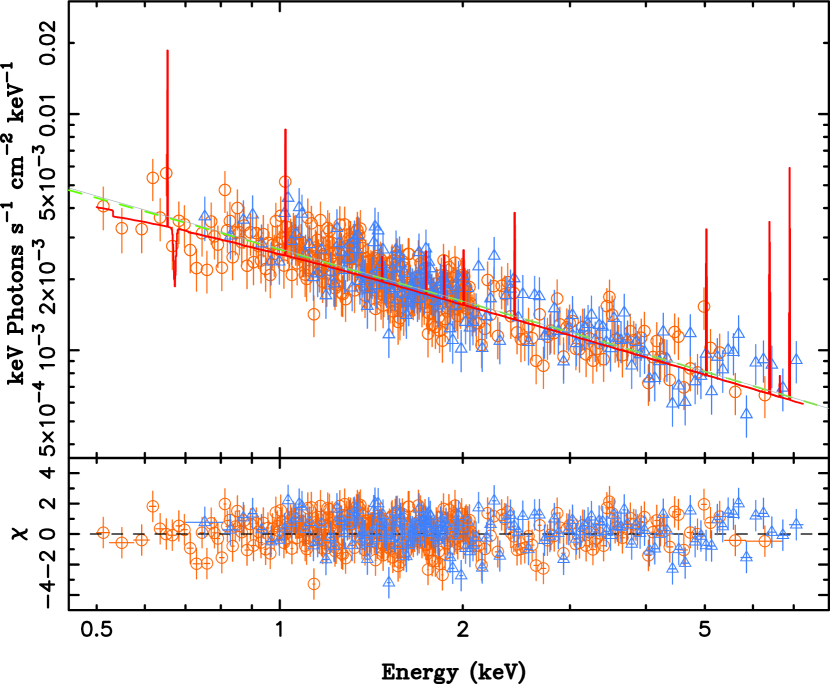
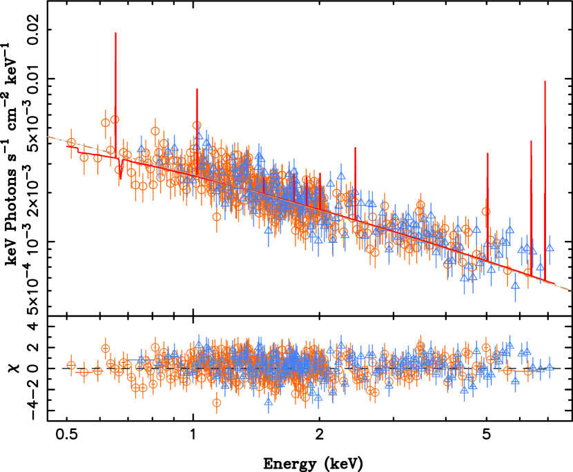
Figure 16: Same as Fig. 15, closeup view of X-ray band. An explanation of the included lines can be found in Young et al. (2007).

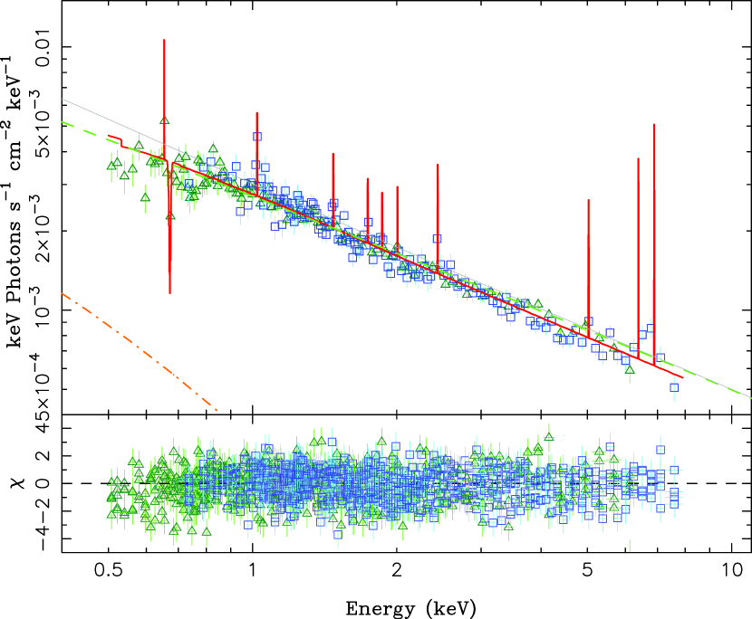
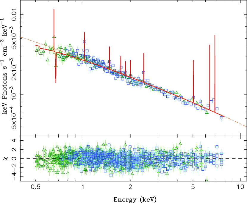
Figure 18: Model fit to combined set of all broadband observations, closeup view of X-ray band. Same symbol/line definitions as Fig. 16.

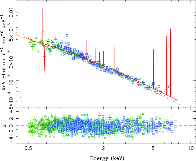
Figure 20: Same as Fig. 19, closeup view of X-ray band. Same symbol/line definitions as Fig. 16

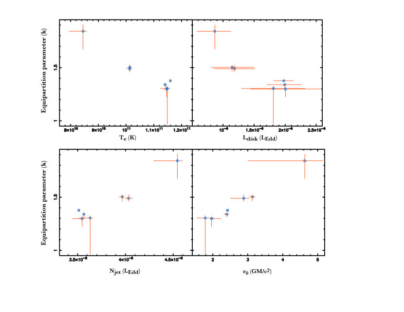
Figure 22: Possible correlations between the magnetic/particle energy density equipartition parameter $k$ and four other fit parameters based on the Maxwellian fits to separate and combined data sets described in Figs. 15–20 and Tables 13–14.

References

- An et al. (2005) An, T., Goss, W. M., Zhao, J.-H., Hong, X. Y., Roy, S., Rao, A. P., & Shen, Z.-Q. 2005, ApJ, 634, L49
- Baganoff (2003) Baganoff, F. K. 2003, AAS/High Energy Astrophysics Division, 7,
- Baganoff et al. (2001) Baganoff, F. K., Bautz, M. W., Brandt, W. N., Chartas, G., Feigelson, E. D., Garmire, G. P., Maeda, Y., Morris, M., Ricker, G. R., Townsley, L. K., & Walter, F. 2001, Nature, 413, 45
- Baganoff et al. (2003) Baganoff, F. K., Maeda, Y., Morris, M., Bautz, M. W., Brandt, W. N., & Burrows, D. N. 2003, ApJ, 591, 891
- Beloborodov (1999) Beloborodov, A. M. 1999, ApJ, 510, L123
- Bietenholz et al. (2000) Bietenholz, M. F., Bartel, N., & Rupen, M. P. 2000, ApJ, 532, 895
- Blandford & Begelman (1999) Blandford, R. D., & Begelman, M. C. 1999, MNRAS, 303, L1
- Blandford & Königl (1979) Blandford, R. D., & Königl, A. 1979, ApJ, 232, 34
- Bower et al. (1996) Bower, G. A., Wilson, A. S., Heckman, T. M., & Richstone, D. O. 1996, AJ, 111, 1901
- Bower et al. (2002) Bower, G. C., Falcke, H., Sault, R. J., & Backer, D. C. 2002, ApJ, 571, 843
- Bower et al. (2005) Bower, G. C., Falcke, H., Wright, M. C., & Backer, D. C. 2005, ApJ, 618, L29
- Bower et al. (2003) Bower, G. C., Wright, M. C. H., Falcke, H., & Backer, D. C. 2003, ApJ, 588, 331
- Brunthaler et al. (2006) Brunthaler, A., Bower, G. C., & Falcke, H. 2006, A&A, 451, 845
- Brunthaler et al. (2001) Brunthaler, A., Bower, G. C., Falcke, H., & Mellon, R. R. 2001, ApJ, 560, L123
- Canizares et al. (2005) Canizares, C. R., Davis, J. E., Dewey, D., Flanagan, K. A., Galton, E. B., Huenemoerder, D. P., Ishibashi, K., Markert, T. H., Marshall, H. L., McGuirk, M., Schattenburg, M. L., Schulz, N. S., Smith, H. I., & Wise, M. 2005, PASP, 117, 1144
- Chandra et al. (2004) Chandra, P., Ray, A., & Bhatnagar, S. 2004, ApJ, 612, 974
- Chary et al. (2000) Chary, R., Becklin, E. E., Evans, A. S., Neugebauer, G., Scoville, N. Z., Matthews, K., & Ressler, M. E. 2000, ApJ, 531, 756
- Devereux et al. (2003) Devereux, N., Ford, H., Tsvetanov, Z., & Jacoby, G. 2003, AJ, 125, 1226
- Done et al. (2007) Done, C., Gierliński, M., & Kubota, A. 2007, A&A Rev., 15, 1
- Eckart et al. (2004) Eckart, A., Baganoff, F. K., Morris, M., Bautz, M. W., Brandt, W. N., Garmire, G. P., Genzel, R., Ott, T., Ricker, G. R., Straubmeier, C., Viehmann, T., Schödel, R., Bower, G. C., & Goldston, J. E. 2004, A&A, 427, 1
- Eckart et al. (2006a) Eckart, A., Baganoff, F. K., Schödel, R., Morris, M., Genzel, R., Bower, G. C., et al. 2006a, A&A, 450, 535
- Eckart et al. (2006b) Eckart, A., Schödel, R., Meyer, L., Trippe, S., Ott, T., & Genzel, R. 2006b, A&A, 455, 1
- Falcke (1996) Falcke, H. 1996, ApJ, 464, L67
- Falcke et al. (2004) Falcke, H., Körding, E., & Markoff, S. 2004, A&A, 414, 895
- Falcke & Markoff (2000) Falcke, H., & Markoff, S. 2000, A&A, 362, 113
- Fender (2006) Fender, R. 2006, Jets from X-ray binaries (Compact stellar X-ray sources), 381–419
- Fender et al. (2003) Fender, R. P., Gallo, E., & Jonker, P. G. 2003, MNRAS, 343, L99
- Freedman et al. (1994) Freedman, W. L., Hughes, S. M., Madore, B. F., Mould, J. R., Lee, M. G., Stetson, P., Kennicutt, R. C., Turner, A., Ferrarese, L., Ford, H., Graham, J. A., Hill, R., Hoessel, J. G., Huchra, J., & Illingworth, G. D. 1994, ApJ, 427, 628
- Gallo et al. (2007) Gallo, E., Migliari, S., Markoff, S., Tomsick, J., Bailyn, C., Berta, S., Fender, R., & Miller-Jones, J. 2007, ApJ, in press (astro-ph/0707.0028)
- Gordon et al. (2004) Gordon, K. D., Pérez-González, P. G., Misselt, K. A., Murphy, E. J., et al. 2004, ApJS, 154, 215
- Grossan et al. (2001) Grossan, B., Gorjian, V., Werner, M., & Ressler, M. 2001, ApJ, 563, 687
- Heckman (1980) Heckman, T. M. 1980, A&A, 87, 152
- Ho (1999) Ho, L. C. 1999, ApJ, 516, 672
- Ho et al. (1996) Ho, L. C., Filippenko, A. V., & Sargent, W. L. W. 1996, ApJ, 462, 183
- Ho et al. (1999) Ho, L. C., van Dyk, S. D., Pooley, G. G., Sramek, R. A., & Weiler, K. W. 1999, AJ, 118, 843
- Ho et al. (2004) Ho, P. T. P., Moran, J. M., & Lo, K. Y. 2004, ApJ, 616, L1
- Houck (2002) Houck, J. C. 2002, in High Resolution X-ray Spectroscopy with XMM-Newton and Chandra
- Immler & Wang (2001) Immler, S., & Wang, Q. D. 2001, ApJ, 554, 202
- Iyomoto & Makishima (2001) Iyomoto, N., & Makishima, K. 2001, MNRAS, 321, 767
- Jokipii (1987) Jokipii, J. R. 1987, ApJ, 313, 842
- Koide et al. (2000) Koide, S., Meier, D. L., Shibata, K., & Kudoh, T. 2000, ApJ, 536, 668
- Körding et al. (2006) Körding, E., Falcke, H., & Corbel, S. 2006, A&A, 456, 439
- La Parola et al. (2004) La Parola, V., Fabbiano, G., Elvis, M., Nicastro, F., Kim, D. W., & Peres, G. 2004, ApJ, 601, 831
- Liu & Melia (2001) Liu, S., & Melia, F. 2001, ApJ, 561, L77
- Malzac et al. (2001) Malzac, J., Beloborodov, A. M., & Poutanen, J. 2001, MNRAS, 326, 417
- Maoz et al. (2005) Maoz, D., Nagar, N. M., Falcke, H., & Wilson, A. S. 2005, ApJ, 625, 699
- Markoff (2005) Markoff, S. 2005, ApJ, 618, L103
- Markoff et al. (2007) Markoff, S., Bower, G. C., & Falcke, H. 2007, MNRAS, in press (astro-ph/0702637)
- Markoff et al. (2001a) Markoff, S., Falcke, H., & Fender, R. 2001a, A&A, 372, L25
- Markoff et al. (2001b) Markoff, S., Falcke, H., Yuan, F., & Biermann, P. L. 2001b, A&A, 379, L13
- Markoff et al. (2003) Markoff, S., Nowak, M., Corbel, S., Fender, R., & Falcke, H. 2003, A&A, 397, 645
- Markoff et al. (2005) Markoff, S., Nowak, M. A., & Wilms, J. 2005, ApJ, 635, 1203
- Merloni & Fabian (2002) Merloni, A., & Fabian, A. C. 2002, MNRAS, 332, 165
- Merloni et al. (2003) Merloni, A., Heinz, S., & di Matteo, T. 2003, MNRAS, 345, 1057
- Meyer & Meyer-Hofmeister (1994) Meyer, F., & Meyer-Hofmeister, E. 1994, A&A, 288, 175
- Meyer et al. (2007) Meyer, L., Schödel, R., Eckart, A., Duschl, W. J., Karas, V., & Dovciak, M. 2007, A&A, submitted
- Migliari et al. (2007) Migliari, S., Tomsick, J. A., Markoff, S., Kalemci, E., Bailyn, C., Buxton, M., Corbel, S., Fender, R. P., & Kaaret, P. 2007, ApJ, in press
- Murphy et al. (2006) Murphy, E. J., Braun, R., Helou, G., Armus, L., Kenney, J. D. P., Gordon, K. D., Bendo, G. J., Dale, D. A., Walter, F., Oosterloo, T. A., Kennicutt, R. C., Calzetti, D., Cannon, J. M., Draine, B. T., Engelbracht, C. W., Hollenbach, D. J., Jarrett, T. H., Kewley, L. J., Leitherer, C., Li, A., Meyer, M. J., Regan, M. W., Rieke, G. H., Rieke, M. J., Roussel, H., Sheth, K., Smith, J. D. T., & Thornley, M. D. 2006, ApJ, 638, 157
- Narayan et al. (1998) Narayan, R., Mahadevan, R., Grindlay, J. E., Popham, R. G., & Gammie, C. 1998, ApJ, 492, 554
- Narayan & Yi (1994) Narayan, R., & Yi, I. 1994, ApJ, 428, L13
- Page et al. (2003) Page, M. J., Breeveld, A. A., Soria, R., Wu, K., Branduardi-Raymont, G., Mason, K. O., Starling, R. L. C., & Zane, S. 2003, A&A, 400, 145
- Pellegrini et al. (2000) Pellegrini, S., Cappi, M., Bassani, L., Malaguti, G., Palumbo, G. G. C., & Persic, M. 2000, A&A, 353, 447
- Quataert & Gruzinov (1999) Quataert, E., & Gruzinov, A. 1999, ApJ, 520, 248
- Remillard & McClintock (2006) Remillard, R. A., & McClintock, J. E. 2006, ARA&A, 44, 49
- Rykoff et al. (2007) Rykoff, E. S., Miller, J. M., Steeghs, D., & Torres, M. A. P. 2007, ApJ, submitted (astro-ph/0703497)
- Sakamoto et al. (2001) Sakamoto, K., Fukuda, H., Wada, K., & Habe, A. 2001, AJ, 122, 1319
- Satyapal et al. (2005) Satyapal, S., Dudik, R. P., O’Halloran, B., & Gliozzi, M. 2005, ApJ, 633, 86
- Schödel et al. (2007) Schödel, R., Krips, M., Markoff, S., Neri, R., & Eckart, A. 2007, A&A, 463, 551
- Shakura & Sunyaev (1973) Shakura, N. I., & Sunyaev, R. A. 1973, A&A, 24, 337
- Swarup et al. (1991) Swarup, G., Ananthakrishnan, S., Kapahi, V. K., Rao, A. P., Subrahmanya, C. R., & Kulkarni, V. K. 1991, CURRENT SCIENCE V.60, NO.2/JAN25, P. 95, 1991, 60, 95
- van der Laan (1966) van der Laan, H. 1966, Nature, 211, 1131
- Willner et al. (2004) Willner, S. P., Ashby, M. L. N., Barmby, P., Fazio, G. G., Pahre, M., Smith, H. A., Kennicutt, R. C., Calzetti, D., Dale, D. A., Draine, B. T., Regan, M. W., Malhotra, S., Thornley, M. D., Appleton, P. N., Frayer, D., Helou, G., Stolovy, S., & Storrie-Lombardi, L. 2004, ApJS, 154, 222
- Wilms et al. (2006) Wilms, J., Nowak, M. A., Pottschmidt, K., Pooley, G. G., & Fritz, S. 2006, A&A, 447, 245
- Young et al. (2007) Young, A. J., Nowak, M. A., Markoff, S., Marshall, H. L., & et al., C. C. R. 2007, ApJ, submitted
- Yuan et al. (2002) Yuan, F., Markoff, S., Falcke, H., & Biermann, P. L. 2002, A&A, 391, 139
- Yuan et al. (2003) Yuan, F., Quataert, E., & Narayan, R. 2003, ApJ, 598, 301
- Yusef-Zadeh et al. (2006) Yusef-Zadeh, F., Bushouse, H., Dowell, C. D., Wardle, M., Roberts, D., Heinke, C., Bower, G. C., Vila-Vilaró, B., Shapiro, S., Goldwurm, A., & Bélanger, G. 2006, ApJ, 644, 198