On the Convexity of the MSE Region of Single-Antenna Users

Abstract

We prove convexity of the sum-power constrained mean square error (MSE) region in case of two single-antenna users communicating with a multi-antenna base station. Due to the MSE duality this holds both for the vector broadcast channel and the dual multiple access channel. Increasing the number of users to more than two, we show by means of a simple counter-example that the resulting MSE region is not necessarily convex any longer, even under the assumption of single-antenna users. In conjunction with our former observation that the two user MSE region is not necessarily convex for two multi-antenna users, this extends and corrects the hitherto existing notion of the MSE region geometry.

I Introduction

Up to now, only few contributions on the geometrical structure of the mean square error region exist. In [1], the authors show that the multi-user MIMO MSE region is convex under fixed transmit and receive beamforming vectors both for linear and nonlinear preprocessing. Obviously, a larger set of MSE tuples can be achieved by means of adaptive transmit and receive beamformers. For this extended setup only the two user case has been investigated so far. Utilizing matrix inequalities of matrix-convex functions, the authors in [2] prove that the two user multi-antenna MSE region cannot exhibit a nonconvex dent between two feasible MSE points connected by a line segment with $-45^{\circ}$ slope. From this observation, they claim that the MSE region is convex. For convexity, however, all possible slopes would have to be checked. As a matter of fact, a channel realization exhibiting a nonconvex MSE region with two multi-antenna users has been observed in [3] disproving the convexity theorem in [2]. A multi-carrier system where several single-antenna users communicate with a single-antenna base station has been investigated in [4]. There, the complementary MSE region of parallel broadcast channels is shown to be not necessarily convex. Since the system under consideration in [4] can be recast into a block diagonal MIMO broadcast channel, the authors of [4] conclude that the two user multi-antenna MSE region cannot be convex in general which again contradicts the theorem in [2]. So far, no distinct statements on convexity of the MSE region depending on the number of users and antennas per user are available in case of adaptive transmit and receive beamformers.

Some applications for which the geometry of the MSE region is of interest are for example the stream priorization according to buffer states or queue states by means of the weighted sum-MSE minimization, cf. [5]. Here, suboptimum transmit and receive filters are derived by repeatedly switching between the downlink and the dual uplink in combination with a geometric program solver for a reasonable power allocation. Balancing is considered in [6] where the weights of a weighted sum-MSE minimization are adapted until certain MSE ratios hold. Exploiting the relationship between the derivative of the the mutual information and the minimum mean square error, Christensen et al. tackle the weighted sum-rate maximization utilizing results from a weighted sum-MSE minimization, see [7]. However, convexity of the MSE region is the crucial point for the proper functionality of above applications since nonconvexity may for example prevent convergence of iterative algorithms. Finally, the MSE $\varepsilon$ achieved with MMSE receivers is tightly related to the maximum SINR via

$$\mathrm{SINR}=\frac{1}{\varepsilon}-1,\\$$ (1)

and hence, also to the data rate $R$ via the simple relation

$$R=-\log_{2}\varepsilon.$$ (2)

Summing up, all this clearly motivates a detailed investigation.

In this paper, we extend the hitherto existing notion of the MSE region geometry. The single antenna case with two users is covered in Section II whereas statements on the convexity of the MSE region for three or more single-antenna users are presented in Section III. Finally, a conjecture on the convexity of the multi-antenna two user case is given in Section IV, and detailed proofs for the theorems and corollaries are attached in Appendices A–C for the sake of readability.

II Convexity for Two Single-Antenna Users

In this section we present statements on the geometry of the MSE region of two single-antenna users. For this setup, convexity can always be shown:

 

Theorem II.1:

The MSE region of two single-antenna users is convex both in the multiple-access channel and in the vector broadcast channel.  

Proof:

See Appendix A.

For the most important part of the boundary of the two user MSE region (see Fig. 1) there is a functional relationship

$$\varepsilon_{2}=g(\varepsilon_{1})$$ (3)

between the two users’ MSEs $\varepsilon_{1}$ and $\varepsilon_{2}$. If the channel vectors $\mathbit{h}_{1}$ and $\mathbit{h}_{2}$ describing the transmission from both users to the base station in the dual MAC are not colinear, the function $g$ is strictly convex, otherwise, it is affine:

 

Corollary II.1.

The function $g:\varepsilon_{1}\mapsto\varepsilon_{2}=g(\varepsilon_{1})$ describing the efficient set of the MSE region is strictly convex if $\mathbit{h}_{1}$ and $\mathbit{h}_{2}$ are not colinear. Otherwise, $g$ is affine.  

Proof:

See Appendix B.

III Nonconvexity Example for More than Two Single-Antenna Users

Although the MSE region is convex for two single-antenna users, this property may get lost when adding an additional user, even if he is equipped with only a single antenna:

 

Theorem III.1:

The three user MSE region of both the vector broadcast channel and the multiple-access channel is not necessarily convex.  

Proof:

For the proof, we present a simple example in Appendix C where the line segment connecting two feasible MSE triples lies outside the MSE region. A further confirmation of Theorem III.1 results from the observation, that the weighted sum-MSE minimization has more than one local minimum, see Appendix C.

Nonconvexity implies for example that not every point of the MSE efficient set can be achieved by means of the weighted sum-MSE minimization technique. Balancing approaches based on the weighted sum-MSE minimization algorithm hence may fail to achieve the desired MSE ratios, cf. [3]. Instead they are prone to oscillations. The following theorem covers the case when (three or) more than three users are present in the system:

 

Theorem III.2:

The MSE region of more than two users may be nonconvex both in the vector broadcast channel and in the multiple-access channel.  

\psfrag{1}{$1$}\psfrag{e2}{$\varepsilon_{2}$}\psfrag{e1}{$\varepsilon_{1}$}\psfrag{e2min}{$\varepsilon_{\text{min},2}$}\psfrag{e1min}{$\varepsilon_{\text{min},1}$}\psfrag{g}{{\small$\varepsilon_{2}=g(\varepsilon_{1})$}}\includegraphics[width=144.54pt]{function_g.eps}

Figure 1: MSE $\varepsilon_{2}$ of user $2$ depending on MSE $\varepsilon_{1}$ of user $1$.

Proof:

The three user case has already been shown in Theorem III.1. For more than three users, the MSE region is a multi-dimensional manifold. However, setting the powers of those users to $p_{4}=\ldots=p_{K}=0$, the intersection of this manifold with the $K-3$ hyperplane(s) $p_{i}=0,\ i\in\{4,\ldots,K\}$, is again a three-dimensional manifold which may have the same geometry as the manifold of the three user case. Hence, the MSE region may be nonconvex for more than three users as well.

IV Conjecture on the Convexity of the Multi-Antenna Two User Case

A counter-example to convexity of the MSE region when multi-antenna users are involved has been shown in [3], where two users each equipped with two antennas communicate with a multi-antenna base-station. Similarly, the multi-carrier single-antenna system in [4] can be recast into a multi-antenna MIMO broadcast channel system where again nonconvexity was observed. Following the idea in the proof of Theorem III.2, the MSE region of two or more than two users may be nonconvex as soon as two multi-antenna users are present. Proving convexity for the case of one single-antenna user and one multi-antenna user turns out to be difficult since a parametrization of the lower left boundary of the feasible MSE region is not known, points on this boundary are obtained by limits of iterative algorithms. Nonetheless, extensive simulation results bring us to the conjecture that the MSE region of one single antenna user and one multi-antenna user is convex.

Appendix A Proof of Theorem II.1

Because of the MSE duality between the vector BC [8] and the MAC in [9, 6, 10], it suffices to prove convexity in the MAC which is easier to handle. Fig. 1 shows the basic characteristics of the two user MSE region for single-antenna users. Here, the MSEs $\varepsilon_{1}$ and $\varepsilon_{2}$ of both users are upper bounded by $1$ since MMSE receivers are assumed. Allowing for other receiver types does not bring any reasonable gain since only MSE-pairs where at least one entry may lie above $1$ would arise. Under the assumption of MMSE receivers, the right part of the boundary of the MSE region is obtained when user one does not transmit any data to the base station at all and user two varies its transmit power from zero to $P_{\mathrm{Tx}}$. Similarly, the upper part of the boundary is reached when user two does not transmit at all whereas user one varies its transmit power from zero to $P_{\mathrm{Tx}}$. Evidently, the most interesting part of the boundary is the lower left one, where the sum of both transmit powers equals the maximum available power $P_{\mathrm{Tx}}$. MSE pairs lying on this boundary feature the functional relationship $\varepsilon_{2}=g(\varepsilon_{1})$, where the domain and the image of $g$ are the sets $[\varepsilon_{\text{min},1},1]$ and $[\varepsilon_{\text{min},2},1]$, respectively. When less than the total transmit power $P_{\mathrm{Tx}}$ is consumed, points are achieved that are element of the interior of the MSE region. As a conclusion, convexity of the set of feasible MSE points corresponds to convexity of the function $g$ relating the MSE $\varepsilon_{1}$ of user one to the MSE $\varepsilon_{2}$ of user two on the lower left boundary of the MSE region. In the following, we show that

$$\frac{\partial^{2}\varepsilon_{2}}{\partial\varepsilon_{1}^{2}}=\frac{\partial^{2}g(\varepsilon_{1})}{\partial\varepsilon_{1}^{2}}\geq 0$$ (4)

holds which immediately implies convexity of $g$.

Unfortunately, a direct functional relationship between $\varepsilon_{2}$ and $\varepsilon_{1}$ is not available. Instead, the two MSEs $\varepsilon_{1}$ and $\varepsilon_{2}$ are parametrized by the transmit power of one of them, for example by the transmit power $p\in\mathbb{D}=[0,P_{\mathrm{Tx}}]$ of user one:

$$\varepsilon_{1}=f_{1}(p),\quad\varepsilon_{2}=f_{2}(p).$$

We can conclude that user two has to transmit with power $P_{\mathrm{Tx}}-p$ in order to utilize the complete power budget. In conjunction with MMSE receivers, the mean square error of user one reads as

$$\varepsilon_{1}=f_{1}(p)=1-p\mathbit{h}_{1}^{\operatorname{H}}\mathbit{X}^{-1}(p)\mathbit{h}_{1}>0,$$ (5)

with the positive definite covariance matrix of the received signal

$$\mathbit{X}(p)=\sigma_{\eta}^{2}\mathbf{I}_{N}+p\mathbit{h}_{1}\mathbit{h}_{1}^{\operatorname{H}}+(P_{\mathrm{Tx}}-p)\mathbit{h}_{2}\mathbit{h}_{2}^{\operatorname{H}}$$ (6)

and $\sigma_{\eta}^{2}>0$ represents the variance of the noise at every antenna element. Similarly, the MSE of user two is denoted by

$$\varepsilon_{2}=f_{2}(p)=1-(P_{\mathrm{Tx}}\!-\!p)\mathbit{h}_{2}^{\operatorname{H}}\mathbit{X}^{-1}(p)\mathbit{h}_{2}>0.$$ (7)

Combining (5), (7), and (6), the function $f_{1}$ turns out to be strictly monotonically decreasing in $p$, i.e.,

$$\dot{\varepsilon}_{1}:=\frac{\partial f_{1}(p)}{\partial p}<0\quad\forall p\in\mathbb{D},$$ (8)

whereas $f_{2}$ is strictly monotonically increasing in $p$:

$$\dot{\varepsilon}_{2}:=\frac{\partial f_{2}(p)}{\partial p}>0\quad\forall p\in\mathbb{D}.$$ (9)

From (8) and (9), pseudo-convexity of $g$ already follows. Before validating (4), we compute the first derivative:

$$\frac{\partial g(\varepsilon_{1})}{\partial\varepsilon_{1}}=\left.\frac{\frac{\partial f_{2}(p)}{\partial p}}{\frac{\partial f_{1}(p)}{\partial p}}\right|_{p=f_{1}^{-1}(\varepsilon_{1})}.$$ (10)

Note that $f_{1}^{-1}(\varepsilon_{1})$ denotes the inverse function of $f_{1}$ which exists due to (8). Differentiating (10) again with respect to $\varepsilon_{1}$ yields

$$\begin{split}\frac{\partial^{2}g(\varepsilon_{2})}{\partial\varepsilon_{1}^{2}}&=\frac{\partial}{\partial\varepsilon_{1}}\Bigg{(}\left.\frac{\frac{\partial f_{2}(p)}{\partial p}}{\frac{\partial f_{1}(p)}{\partial p}}\right|_{p=f_{1}^{-1}(\varepsilon_{1})}\Bigg{)}\\ &=\left.\Bigg{(}\frac{\partial}{\partial p}\ \frac{\frac{\partial f_{2}(p)}{\partial p}}{\frac{\partial f_{1}(p)}{\partial p}}\Bigg{)}\right|_{p=f_{1}^{-1}(\varepsilon_{1})}\cdot\frac{\partial f_{1}^{-1}(\varepsilon_{1})}{\partial\varepsilon_{1}}\\ &=\left.\frac{\ddot{\varepsilon}_{2}\dot{\varepsilon}_{1}-\ddot{\varepsilon}_{1}\dot{\varepsilon}_{2}}{\left(\dot{\varepsilon}_{1}\right)^{2}}\right|_{p=f_{1}^{-1}(\varepsilon_{1})}\cdot\frac{1}{\dot{\varepsilon}_{1}|_{p=f_{1}^{-1}(\varepsilon_{1})}}\\ &=\left.\frac{\ddot{\varepsilon}_{2}\dot{\varepsilon}_{1}-\ddot{\varepsilon}_{1}\dot{\varepsilon}_{2}}{\left(\dot{\varepsilon}_{1}\right)^{3}}\right|_{p=f_{1}^{-1}(\varepsilon_{1})}.\end{split}$$ (11)

Since $f^{-1}_{1}$ maps from $[\varepsilon_{\text{min},1},1]$ to $\mathbb{D}$, and since $\dot{\varepsilon}_{1}<0$ holds $\forall p\in\mathbb{D}$, the function $g$ is convex iff [see (11) and cond. (4)]

$$\ddot{\varepsilon}_{2}\dot{\varepsilon}_{1}-\ddot{\varepsilon}_{1}\dot{\varepsilon}_{2}\leq 0\Leftrightarrow g\ \text{is convex}.$$ (12)

For notational brevity, we introduce the two substitutions

$$a_{i,j}=\mathbit{h}_{i}^{\operatorname{H}}\mathbit{X}^{-1}(p)\mathbit{h}_{j}\quad\text{and}\quad b_{i,j}=\mathbit{h}_{i}^{\operatorname{H}}\mathbit{X}^{-2}(p)\mathbit{h}_{j},$$ (13)

which satisfy $a_{i,j}=a_{j,i}^{*}$ and $b_{i,j}=b_{j,i}^{*}$. Making use of

$$\frac{\partial\mathbit{X}^{-1}(p)}{\partial p}=-\mathbit{X}^{-1}(p)\frac{\partial\mathbit{X}(p)}{\partial p}\mathbit{X}^{-1}(p),$$

the first derivatives with respect to $p$ in (8) and (9) can be shown to equal

$$\begin{split}\dot{\varepsilon}_{1}&=-\sigma_{\eta}^{2}b_{1,1}-P_{\mathrm{Tx}}|a_{1,2}|^{2},\\ \dot{\varepsilon}_{2}&=+\sigma_{\eta}^{2}b_{2,2}+P_{\mathrm{Tx}}|a_{1,2}|^{2},\end{split}$$ (14)

respectively. Differentiating (14) again w.r.t. $p$, we obtain

$$\begin{split}\ddot{\varepsilon}_{1}=2\sigma_{\eta}^{2}[a_{1,1}b_{1,1}-\Re\{a_{1,2}b_{2,1}\}]+2P_{\mathrm{Tx}}|a_{1,2}|^{2}(a_{1,1}-a_{2,2}),\\ \ddot{\varepsilon}_{2}=2\sigma_{\eta}^{2}[a_{2,2}b_{2,2}-\Re\{a_{2,1}b_{1,2}\}]+2P_{\mathrm{Tx}}|a_{1,2}|^{2}(a_{2,2}-a_{1,1}).\end{split}$$

Inserting (14) and the last two equations into (12) and applying $\Re\{a_{2,1}b_{1,2}\}=\Re\{a_{1,2}b_{2,1}\}$ results in

$$\begin{split}&\ddot{\varepsilon}_{2}\dot{\varepsilon}_{1}-\ddot{\varepsilon}_{1}\dot{\varepsilon}_{2}=\\ &\ \ \ 2\sigma_{\eta}^{2}P_{\mathrm{Tx}}|a_{1,2}|^{2}\left[2\Re\{a_{1,2}b_{2,1}\}-a_{2,2}b_{1,1}-a_{1,1}b_{2,2}\right]\\ &\ \ \ +2\sigma_{\eta}^{4}b_{1,1}\left(\Re\{a_{1,2}b_{2,1}\}-a_{1,1}b_{2,2}\right)\\ &\ \ \ +2\sigma_{\eta}^{4}b_{2,2}\left(\Re\{a_{1,2}b_{2,1}\}-a_{2,2}b_{1,1}\right).\end{split}$$ (15)

In order to prove that (15) is not positive to fulfill the convexity requirement in (12), we will reveal that all three summands in (15) are not positive.

For the first summand, this turns out to be very easy: Noticing that $a_{i,i}>0$ and $b_{i,i}>0$, the first summand in (15) is nonpositive if

$$4\Re^{2}\{a_{2,1}b_{1,2}\}\leq(a_{2,2}b_{1,1}+a_{1,1}b_{2,2})^{2}.$$ (16)

Clearly, we can upper bound the real part by the magnitude and apply the Cauchy-Schwarz-inequality with (13) to bound the magnitude:

$$4\Re^{2}\{a_{2,1}b_{1,2}\}\leq 4|a_{2,1}b_{1,2}|^{2}\leq 4a_{2,2}a_{1,1}b_{1,1}b_{2,2}.$$ (17)

Validating the inequality

$$\begin{split}(a_{2,2}b_{1,1}+a_{1,1}b_{2,2})^{2}&\geq 4a_{2,2}a_{1,1}b_{1,1}b_{2,2}\\ \Leftrightarrow(a_{2,2}b_{1,1}-a_{1,1}b_{2,2})^{2}&\geq 0\end{split}$$

leads in conjunction with (17) to the conclusion that (16) is fulfilled, i.e., the first summand in (15) is nonpositive.

Nonpositivity of the second summand in (15) is resembled by the inequality

$$\Re\left\{\frac{a_{1,2}}{a_{1,1}}\frac{b_{2,1}}{b_{2,2}}\right\}\leq 1.$$ (18)

To prove (18) we explicitly have to exploit the structure of $\mathbit{X}(p)$ in (6) which makes the proof longer than the one for the first summand. Interestingly, the real part operator in (18) is redundant as its argument turns out to be real-valued. Applying the matrix inversion lemma several times, we get

$$\frac{a_{1,2}}{a_{1,1}}=\frac{\sigma_{\eta}^{2}\mathbit{h}_{1}^{\operatorname{H}}\mathbit{h}_{2}}{\sigma_{\eta}^{2}\|\mathbit{h}_{1}\|_{2}^{2}+d(P_{\mathrm{Tx}}\!-\!p)},$$ (19)

with the substitution

$$d=\|\mathbit{h}_{1}\|_{2}^{2}\|\mathbit{h}_{2}\|_{2}^{2}\!-\!|\mathbit{h}_{1}^{\operatorname{H}}\mathbit{h}_{2}|^{2}\geq 0.$$ (20)

Applying several times the matrix inversion lemma as for the first fraction, the second fraction in (18) can be expressed as

$$\frac{b_{2,1}}{b_{2,2}}=\frac{\mathbit{h}_{2}^{\operatorname{H}}\mathbit{h}_{1}\left[\sigma_{\eta}^{4}-p(P_{\mathrm{Tx}}\!-\!p)d\right]}{\sigma_{\eta}^{4}\|\mathbit{h}_{2}\|_{2}^{2}+dp(2\sigma_{\eta}^{2}+p\|\mathbit{h}_{1}\|_{2}^{2})}.$$ (21)

Multiplying (19) by (21) yields the real-valued expression

$$\frac{b_{2,1}a_{1,2}}{a_{1,1}b_{2,2}}=\frac{\sigma_{\eta}^{6}|\mathbit{h}_{1}^{\operatorname{H}}\mathbit{h}_{2}|^{2}-c_{1}}{\sigma_{\eta}^{6}\|\mathbit{h}_{1}\|_{2}^{2}\|\mathbit{h}_{2}\|_{2}^{2}+c_{2}}\ \in\mathbb{R}$$

with the two substitutions

$$\begin{split}c_{1}&=\sigma_{\eta}^{2}|\mathbit{h}_{1}^{\operatorname{H}}\mathbit{h}_{2}|^{2}pd(P_{\mathrm{Tx}}-p)\geq 0,\\ c_{2}&=\left[\sigma_{\eta}^{2}\|\mathbit{h}_{1}\|_{2}^{2}+d(P_{\mathrm{Tx}}-p)\right]dp\left(2\sigma_{\eta}^{2}+p\|\mathbit{h}_{1}\|_{2}^{2}\right)\\ &\quad+\sigma_{\eta}^{4}\|\mathbit{h}_{2}\|_{2}^{2}d(P_{\mathrm{Tx}}-p)\geq 0.\end{split}$$

Since both $c_{1}$ and $c_{2}$ are nonnegative, we find

$$\frac{b_{2,1}a_{1,2}}{a_{1,1}b_{2,2}}\leq\frac{\sigma_{\eta}^{6}|\mathbit{h}_{1}^{\operatorname{H}}\mathbit{h}_{2}|^{2}}{\sigma_{\eta}^{6}\|\mathbit{h}_{1}\|_{2}^{2}\|\mathbit{h}_{2}\|_{2}^{2}}$$

as an upper bound from which (18) directly follows due to the Cauchy-Schwarz-inequality. Thus, the nonpositivity of the second summand in (15) is proven.

Finally, the nonpositivity of the third summand in (15) is shown by the same reasoning as for the second summand:

$$\Re\left\{\frac{a_{1,2}}{a_{2,2}}\frac{b_{2,1}}{b_{1,1}}\right\}\leq 1$$ (22)

is deduced from

$$\frac{b_{2,1}a_{1,2}}{a_{2,2}b_{1,1}}=\frac{\sigma_{\eta}^{6}|\mathbit{h}_{1}^{\operatorname{H}}\mathbit{h}_{2}|^{2}-d_{1}}{\sigma_{\eta}^{6}\|\mathbit{h}_{1}\|_{2}^{2}\|\mathbit{h}_{2}\|_{2}^{2}+d_{2}}\ \in\mathbb{R},$$

where $d_{i}$ follows from $c_{i}$ by interchanging indices and powers:

$$\begin{split}d_{1}&=c_{1},\\ d_{2}&=\left(\sigma_{\eta}^{2}\|\mathbit{h}_{2}\|_{2}^{2}+dp\right)d(P_{\mathrm{Tx}}-p)\left[2\sigma_{\eta}^{2}+(P_{\mathrm{Tx}}-p)\|\mathbit{h}_{2}\|_{2}^{2}\right]\\ &\quad+\sigma_{\eta}^{4}\|\mathbit{h}_{1}\|_{2}^{2}dp\geq 0.\end{split}$$

As all three summands in (15) are nonpositive, the inequality in (12) is satisfied and the proof for the convexity of the MSE region is complete.

Appendix B Proof of Corollary II.1

If the inequality in (12) is strict for all $p\in\mathbb{D}$, $g$ is strictly convex. Excluding equality in (12) therefore ensures that $g$ is strictly convex. The difference in (15) is zero if and only if all three summands are zero since each summand is nonpositive. In order to let the first summand vanish, the Cauchy-Schwarz-inequality in (17) has to be fulfilled with equality. To this end, $\mathbit{h}_{1}$ and $\mathbit{h}_{2}$ have to be colinear which also fulfills (16) with equality. If both channel vectors are colinear, $d=0$ results from (20) and the variables $c_{1}$, $c_{2}$, $d_{1}$, and $d_{2}$ are zero as well. Obviously, (18) holds with equality and the last two summands in (15) vanish. Thus, we have shown that if the two channel vectors $\mathbit{h}_{1}$ and $\mathbit{h}_{2}$ are not colinear, then the function $g$ is strictly convex. Additionally, if both vectors are colinear, $g$ has curvature zero for all powers $p\in\mathbb{D}$. As a consequence, $g$ is affine. In the latter case, we have the relationship

$$g(\varepsilon_{1})=-\varepsilon_{1}\frac{|\alpha|^{2}\!+\!|\alpha|^{2}\gamma\|\mathbit{h}_{1}\|_{2}^{2}}{1+|\alpha|^{2}\gamma\|\mathbit{h}_{1}\|_{2}^{2}}+1+\frac{|\alpha|^{2}}{1+|\alpha|^{2}\gamma\|\mathbit{h}_{1}\|_{2}^{2}},$$ (23)

where $\gamma=P_{\mathrm{Tx}}/\sigma_{\eta}^{2}$ denotes the transmit SNR, $\mathbit{h}_{2}=\alpha\mathbit{h}_{1}$, and $\varepsilon_{1}\in[\varepsilon_{\text{min},1},1]$ with

$$\varepsilon_{\text{min},1}=\frac{1}{1+\gamma\|\mathbit{h}_{1}\|_{2}^{2}}.$$ (24)

Appendix C Proof of Theorem III.1

A nonconvex three user MSE region can for example be obtained by the channel matrix

$$\mathbit{H}=[\mathbit{h}_{1},\mathbit{h}_{2},\mathbit{h}_{3}]=\left[\begin{array}[]{ccc}1&0&1\\ 0&1&1\end{array}\right]$$ (25)

and a transmit power $P_{\mathrm{Tx}}=10$. In this case, the base station is equipped with $N=2$ antennas, and the channel vector $\mathbit{h}_{3}$ is the sum of $\mathbit{h}_{1}$ and $\mathbit{h}_{2}$. Note that the base station has fewer antennas than users are present in the system in this special case. Nonconvexity of the MSE region can also be and has been observed when the channel vectors of all users are linearly independent ($N\geq K$ must hold then). If the MSE region was convex, the line segment between every two feasible MSE triples would have to be a subset of the region. Moreover, the weighted sum-MSE minimization with arbitrary nonnegative weights $\mathbit{w}=[w_{1},\ldots,w_{K}]^{\operatorname{T}}\geq\mathbf{0}_{K},\ \mathbit{w}\neq\mathbf{0}_{K}$ may have stationary points fulfilling the KKT conditions with only one common value of the weighted minimization. In the following, we show that these conditions are violated for the channel in (25).

The weighted sum-MSE minimization reads as

$$\operatorname*{minimize}_{p_{1},\ldots,p_{K}}\sum_{k=1}^{K}w_{k}\varepsilon_{k}\quad\text{s.t.:}\ \sum_{k=1}^{K}p_{k}\leq P_{\mathrm{Tx}},\ \ p_{k}\geq 0\ \forall k,$$ (26)

where $p_{k}$ is the power with which user $k$ transmits in the uplink and the MSE of user $k$ reads as

$$\varepsilon_{k}=1-p_{k}\mathbit{h}_{k}^{\operatorname{H}}\mathbit{X}^{-1}\mathbit{h}_{k}$$ (27)

with the received signal covariance matrix

$$\mathbit{X}=\sigma_{\eta}^{2}\mathbf{I}_{N}+\sum_{\ell=1}^{K}p_{\ell}\mathbit{h}_{\ell}\mathbit{h}_{\ell}^{\operatorname{H}}.$$ (28)

The Lagrangian function associated to (26) reads as

$$L=\sum_{k=1}^{K}w_{k}\varepsilon_{k}+\lambda\Big{(}\sum_{k=1}^{K}p_{k}-P_{\mathrm{Tx}}\Big{)}-\sum_{k=1}^{K}\mu_{k}p_{k}.$$ (29)

Note that the Lagrangian multipliers $\lambda$ and $\mu_{1},\ldots,\mu_{K}$ have to be nonnegative real. If above Lagrangian $L$ has stationary points with different values for $L$, the underlying MSE region is not convex since more than one hyperplane with normal vector $[w_{1},\ldots,w_{K}]^{\operatorname{T}}$ locally supporting the MSE region exists. The KKT conditions read as

$$\mathbit{h}_{k}^{\operatorname{H}}\check{\mathbit{X}}^{-1}(w_{k}\check{\mathbit{X}}-\check{\mathbit{S}})\check{\mathbit{X}}^{-1}\mathbit{h}_{k}=\check{\lambda}-\check{\mu}_{k}\ \forall k,$$ (30)

$$\check{p}_{k}\geq 0\ \forall k,$$ (31)

$$\check{p}_{k}\check{\mu}_{k}=0\ \forall k,$$ (32)

$$\check{\mu}_{k}\geq 0\ \forall k,$$ (33)

$$\sum_{k=1}^{K}\check{p}_{k}\leq P_{\mathrm{Tx}},$$ (34)

$$\check{\lambda}\Big{(}\sum_{k=1}^{K}\check{p}_{k}-P_{\mathrm{Tx}}\Big{)}=0,$$ (35)

$$\check{\lambda}\geq 0,$$ (36)

with the substitution

$$\mathbit{S}=\sum_{\ell=1}^{K}w_{\ell}p_{\ell}\mathbit{h}_{\ell}\mathbit{h}_{\ell}^{\operatorname{H}}.$$ (37)

Note that checked variables $\check{(\cdot)}$ are those which fulfill the KKT conditions. Assuming a weight vector

$$\mathbit{w}=[0.22,0.54,0.24]^{\operatorname{T}},$$ (38)

the weighted sum-MSE minimization (26) features two stationary points satisfying the KKT conditions (30)–(36) for the channel vectors (25) and a transmit power $P_{\mathrm{Tx}}=10$. The first set of primal and dual variables fulfilling the KKTs reads as

$$\begin{split}&\check{\mathbit{p}}{}^{(1)}=[3.6753,\ 6.3247,\ 0]^{\operatorname{T}},\ \ \check{\lambda}{}^{(1)}=0.0101,\\ &\check{\mu}_{1}{}^{(1)}=\check{\mu}_{2}{}^{(1)}=0,\ \ \check{\mu}_{3}{}^{(1)}=0.0266,\end{split}$$ (39)

and achieves a weighted sum-MSE $\sum_{k=1}^{3}w_{k}\check{\varepsilon}_{k}{}^{(1)}=0.36078$. The second set of variables reads as

$$\begin{split}&\check{\mathbit{p}}{}^{(2)}=[0,\ 7.0794,\ 2.9206]^{\operatorname{T}},\ \ \check{\lambda}{}^{(2)}=0.0115,\\ &\check{\mu}_{1}{}^{(2)}=0.007,\ \ \check{\mu}_{2}{}^{(2)}=\check{\mu}_{3}{}^{(2)}=0,\end{split}$$ (40)

and obtains a slightly larger metric $\sum_{k=1}^{3}w_{k}\check{\varepsilon}_{k}{}^{(2)}=0.3828$. The existence of two KKT points with different values algebraically proves the nonconvexity of the MSE region.

A geometrical proof is shown in Fig. 2, where the three-user MSE region for the channel in (25) is plotted with $P_{\mathrm{Tx}}=10$. The two KKT points in (39) and (40) achieve individual MSEs

$$\begin{split}\check{\boldsymbol{\varepsilon}}{}^{(1)}=\big{[}\check{\varepsilon}_{1}{}^{(1)},\check{\varepsilon}_{2}{}^{(1)},\check{\varepsilon}_{3}{}^{(1)}\big{]}^{\operatorname{T}}&=[0.2139,\ 0.1365,\ 1]^{\operatorname{T}},\\ \check{\boldsymbol{\varepsilon}}{}^{(2)}=\big{[}\check{\varepsilon}_{1}{}^{(2)},\check{\varepsilon}_{2}{}^{(2)},\check{\varepsilon}_{3}{}^{(2)}\big{]}^{\operatorname{T}}&=[1,\ 0.1977,\ 0.2335]^{\operatorname{T}}.\end{split}$$ (41)

However, the line segment connecting $\check{\boldsymbol{\varepsilon}}{}^{(1)}$ and $\check{\boldsymbol{\varepsilon}}{}^{(2)}$ does not completely belong to the MSE region, it lies outside the region and touches the boundary of the MSE region at $\check{\boldsymbol{\varepsilon}}{}^{(1)}$ and $\check{\boldsymbol{\varepsilon}}{}^{(2)}$. Evidently, the MSE region cannot be convex.

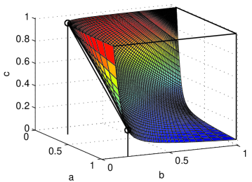
Figure 2: Example of a nonconvex MSE region for $K=3$ users. The line segment connecting two feasible points lies outside the region.

References

- [1] S. Shi and M. Schubert, “Convexity Analysis of the Feasible MSE Region of Sum-Power Constrained Multiuser MIMO Systems,” in Proc. IEEE Internat. Symp. on Personal, Indoor and Mobile Radio Communications (PIMRC), Berlin, Germany, Sept. 2005.
- [2] E. Jorswieck and H. Boche, “Transmission Strategies for the MIMO MAC with MMSE Receiver: Average MSE Optimization and Achievable Individual MSE Region,” IEEE Trans. on Signal Processing, vol. 51, no. 11, pp. 2872–2881, Nov. 2003, special issue on MIMO wireless communications.
- [3] R. Hunger, M. Joham, and W. Utschick, “Efficient MSE Balancing for the Multi-User MIMO Downlink,” in Proc. 41st Asilomar Conference on Signals, Systems, and Computers, November 2007.
- [4] G. Wunder, I. Blau, and T. Michel, “Utility Optimization based on MSE for Parallel Broadcast Channels: The Square Utility Optimization based on MSE for Parallel Broadcast Channels: The Square Root Law,” in 45th Annual Allerton Conference on Communication, Control, and Computing, Monticello, Illinois, September 2007.
- [5] M. Codreanu, A. Tolli, M. Juntti, and M. Latva-aho, “Weighted Sum MSE Minimization for MIMO Broadcast Channel,” in 17th International Symposium on Personal, Indoor, and Mobile Radio Communications (PIMRC), September 2006.
- [6] A. Mezghani, M. Joham, R. Hunger, and W. Utschick, “Transceiver Design for Multi-User MIMO Systems,” in Proc. ITG/IEEE WSA 2006, March 2006.
- [7] S. Christensen, R. Agarwal, E. d. Carvalho, and J. M. Cioffi, “Beamforming Design for Weighted Sum-Rate Maximization in MIMO Broadcast Channels,” Submitted to IEEE Transactions on Wireless Communications.
- [8] W. Yu and J. M. Cioffi, “Sum Capacity of Gaussian Vector Broadcast Channels,” IEEE Trans. Inform. Theory, vol. 50, pp. 1875–1892, September 2004.
- [9] R. Hunger, M. Joham, and W. Utschick, “On the MSE-Duality of the Broadcast Channel and the Multiple Access Channel,” Submitted to IEEE Transactions on Signal Processing.
- [10] M. Schubert, S. Shi, E. A. Jorswieck, and H. Boche, “Downlink Sum-MSE Transceiver Optimization for Linear Multi-User MIMO Systems,” in Proc. Asilomar Conf. on Signals, Systems and Computers, Monterey, CA, Sept. 2005.