Role of scaling in the statistical modeling of finance

Abstract

Modeling the evolution of a financial index as a stochastic process is a problem awaiting a full, satisfactory solution since it was first formulated by Bachelier in 1900. Here it is shown that the scaling with time of the return probability density function sampled from the historical series suggests a successful model. The resulting stochastic process is a heteroskedastic, non-Markovian martingale, which can be used to simulate index evolution on the basis of an auto-regressive strategy. Results are fully consistent with volatility clustering and with the multi-scaling properties of the return distribution. The idea of basing the process construction on scaling, and the construction itself, are closely inspired by the probabilistic renormalization group approach of statistical mechanics and by a recent formulation of the central limit theorem for sums of strongly correlated random variables.

1. Introduction

Economics and mathematical finance are multi-disciplinary fields in which the tendency of statistical physicists to focus on universal laws has been criticized sometimes  [?]. In particular, the emphasis on scaling properties typical of many recent contributions in econophysics has been regarded with skepticism by some economists, in view of the apparent scarcity of useful practical consequences of this symmetry  [?].

As statistical physicists aware of the key role played by scaling and universality in the development of the theory of complex systems in the last decades, we do not share this point of view. Universal laws are necessary for building up our scientific understanding and we do not intend to give them up. In the specific case of scaling symmetries, it is perhaps fair to admit that, so far, their potential consequences in finance have not been fully explored and elucidated  [?]. In the present note we report on recent work  [?] demonstrating that scaling, combined with symmetries enforced by the efficiency of the market, allows substantial progress towards the solution of the central problem of mathematical finance: assuming that the time evolution of a financial index, or asset price, amounts to a stochastic process, formulate a satisfactory model of this process, consistent with as many as possible stylized facts established by the statistical analysis of the historical series  [?,?,?,?,?]. This problem awaits a full, satisfactory solution since it was first formulated by Bachelier  [?].

The approach sketched below points out far reaching consequences of the scaling in time obeyed by the return probability density function sampled from the historical series of an index. These consequences add further strong constraints to those already implied by market efficiency, and suggest very plausible probabilistic rules for the process of index evolution. Our goal here is reached through ideas which are partly inspired by the probabilistic formulation of the renormalization group (RG) in statistical mechanics  [?,?], and by a recent extension of the central limit theorem to sums of strongly correlated variables obeying anomalous scaling  [?]. To our knowledge, renormalization group ideas do not seem to have been applied in mathematical finance so far.

This report is organized as follows. In the second section we recall the basic facts emerging from the statistical analysis of the historical series, taking as example the Dow Jones Industrial (DJI) index. In parallel we also present the core of our derivations and stress their links with renormalization group ideas. In the third section we briefly describe our stochastic model for index evolution, while in the subsequent, fourth one we review the results of the simulation of the DJI index. The last, fifth section is devoted to concluding remarks.

2. Stylized facts and consequences of scaling

Let us indicate by $S(t)$ the value of an index at time $t$. For our purposes here, we can assume that $t$ is measured in days and $S(t)$ represents the daily closure value. A quantity of interest  [?,?,?] is the logarithmic return $r_{t,T}=\ln(S(t+T)-\ln S(t))$ in the interval $[t,t+T]$. The values of $\ln S$ used to compute $r_{t,T}$ are assumed to be detrended, $\ln S(t)\mapsto\ln S(t)-\rho\;t$, where $\rho$ is the average linear growth over the whole time series. A probability density function (PDF) for this return can be sampled from sufficiently long historical time series. The resulting PDF, $p_{T}(r)$, does depend only on $T$. Indeed, being sampled with a sliding interval method, $p_{T}$ conveys only a stationarized information on return occurrences. For $T$’s in the range from one day to few months, $p_{T}$ satisfies approximately simple-scaling: $p_{T}(r)=\frac{1}{T^{D}}g(\frac{r}{T^{D}})$, where the exponent $D$ turns out be very close to $1/2$ for the indexes of well developed markets  [?]. The scaling function $g$, however, is not Gaussian, and shows power law, Pareto tails at large $|r|$  [?]. The scaling of $p_{T}$ in the case of the DJI index is illustrated by the collapse plot in Fig. 1. The non Gaussian form of $g$ indicates that successive returns in the sampling must have strong correlations on the time range where scaling holds. Before mentioning other stylized facts, it is worth concentrating on the scaling of $p_{T}$, which plays a central role in our approach.

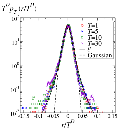
Figure  1.: Scaling collapse of the histograms of return PDF’s of the DJI. Data are sampled over about $26000$ daily closures from 1900 to 2005. The dotted curve is a Gaussian, while the continuous one is the best fit  [?] used here to implement our stochastic model.

In the modern theory of critical phenomena  [?], one can consider a finite block of $N$ interacting spins and try to identify the critical conditions under which doubling the block size ($N\to 2N$) signals the presence of scale invariance in the system. In a phenomenological  [?] version of the probabilistic RG approach  [?], this system doubling can be more simply implemented for hierarchical models in which the Hamiltonian depends only on the total sum, $M$, of the spins. Here the spins, and thus $M$, are assumed to take values in $\mathbb{R}$. The PDF of $M$ in a system of $N$ spins is then indicated by $q_{N}(M)$ and the RG transformation yields $q_{2N}(M)$ as a functional of $q_{N}(M)$, once a suitable interaction between blocks is assumed:

$$q_{2N}(M)=\frac{\int dM_{1}dM_{2}\;e^{H_{I}(M_{1},M_{2})}\;q_{N}(M_{1})\;q_{N}(M_{2})\;\delta(M-M_{1}-M_{2})}{\int dM_{1}dM_{2}\;e^{H_{I}(M_{1},M_{2})}\;q_{N}(M_{1})\;q_{N}(M_{2})}.$$ (1)

In Eq. (1), $H_{I}(M_{1},M_{2})$ is the reduced (divided by $-k_{B}T$) coupling between the magnetizations of the two blocks. The factor multiplying the delta function in the integrand is just the Boltzmann-Gibbs expression of the joint PDF for the magnetizations $M_{1}$ and $M_{2}$ of the two blocks. Fixed-point critical scaling prevails when the interactions are chosen in such a way that Eq. (1) is satisfied by a $q_{N}$ assuming a simple-scaling form $q_{2N}(M)=\frac{1}{2^{D}}q_{N}(\frac{M}{2^{D}})$, where $D$ is now related to the critical exponents of the model.

We can envisage a sort of reverse RG strategy in finance. In analogy with the magnetic case, the scaling of $p_{T}(r)$ can be regarded as a fixed-point scaling for a ‘block’ of $T$ daily returns. So, we can ask what kind of ‘coupling’ must exist between the returns of two successive blocks of duration $T$, in such a way that, as we know, $p_{2T}(r)$ satisfies simple-scaling, i.e. $p_{2T}(r)=\frac{1}{2^{D}}p_{T}(\frac{r}{2^{D}})$. Since there is no Hamiltonian now, the statistical information on this coupling is embodied in the unknown joint PDF of the returns $r_{1}$ and $r_{2}$ in the successive intervals, $p_{2T}^{(2)}(r_{1},r_{2})$. Indeed, since the returns $r_{1}$ and $r_{2}$ sum up to the return in the interval of duration $2T$, this joint PDF satisfies:

$$p_{2T}(r)=\int dr_{1}dr_{2}\;p_{2T}^{(2)}(r_{1},r_{2})\;\delta(r-r_{1}-r_{2}).$$ (2)

One realizes that $r_{1}$ and $r_{2}$ in Eq. (2) play a role analogous to that of $M_{1}$ and $M_{2}$ in Eq. (1). Since $p_{2T}^{(2)}$ is not known, one can imagine to determine this function in terms of $p_{T}$ on the basis of Eq. (2). In the magnetic RG analogy this would amount to determine the critical interaction conditions, once the fixed-point scaling form of $q_{N}(M)$ is given. Of course, this determination is not expected to be unique in general: there can be many different $p_{2T}^{(2)}$’s satisfying Eq. (2) for a given $p_{T}$. However, there are other constraints and symmetries helping in the search of the right solution. A well established empirical fact is that the average $\langle r_{1}r_{2}\rangle_{p_{2T}^{(2)}}\equiv\int dr_{1}dr_{2}\;p_{2T}^{(2)}(r_{1},r_{2})\;r_{1}r_{2}$ must be equal to zero. This can be easily verified and is in fact an obvious requisite for an efficient market. A deviation from zero of this average would open an arbitrage opportunity which would be immediately exploited and suppressed by the market. Other constraints concern the marginal PDF’s:

$$p_{T}(r_{1}) = \int dr_{2}\;p_{2T}^{(2)}(r_{1},r_{2}),$$ (3)

$$p_{T}(r_{2}) = \int dr_{1}\;p_{2T}^{(2)}(r_{1},r_{2}).$$ (4)

The validity of Eqs. (3-4) is based on the fact that both $p_{T}$ and $p_{2T}^{(2)}$ are sampled with a sliding interval method from the historical time series. This marks a difference with respect to the magnetic case, because there the marginal PDF’s would be computed at a rescaled $N$, due to a renormalization effect which is excluded here for the empirical PDF’s of finance. On the basis of Eqs. (2-4) and of the linear decorrelation of successive returns, it is immediate to derive that, for the scaling of $p_{T}$ to occur, one must necessarily have $D=1/2$. It is sufficient to express the average $\langle(r_{1}+r_{2})^{2}\rangle_{p_{2T}^{(2)}}$, and to take into account that the scaling form of $p_{T}$ implies that its second moment must scale as $\langle r^{2}\rangle_{p_{T}}\sim T^{2D}$. One then finds immediately that $2T^{2D}=(2T)^{2D}$, i.e. $D=1/2$. This result explains the robustness of the estimate $D\simeq 1/2$ emerging from the statistical analysis of all indexes in mature markets  [?].

Now let us come back to the problem of expressing $p_{2T}^{(2)}$ in terms of $p_{T}$. If the linear decorrelation of successive returns, i.e. $\langle r_{1}r_{2}\rangle_{p_{2T}^{(2)}}=0$, would imply a complete decorrelation of $r_{1}$ and $r_{2}$, the problem would be easily solved. Indeed, independence would mean $p_{2T}^{(2)}=p_{T}(r_{1})p_{T}(r_{2})$. By substituting in Eq. (2), and using the scaling form of $p_{T}$, we would then conclude immediately that $D=1/2$ and a Gaussian $g(x)=\exp(-x^{2}/2\sigma^{2})/\sqrt{2\pi\sigma^{2}}$ are necessary for consistency. Indeed, in this case of independence Eq. (2) just imposes to $g$ the property of stability which is at the basis of the central limit theorem and is satisfied, for finite variance $\sigma^{2}$, by the Gaussian PDF alone  [?]. This is even more directly verified in terms of characteristic functions (CF). For $p_{T}$ the CF is $\tilde{p}_{T}(k)=\int dre^{ikr}p_{T}(r)=\tilde{g}(T^{D}k)$, and Eq.(2), together with the scaling and the independence conditions, simply reads

$$\tilde{g}((2T)^{D}k)=\tilde{g}(T^{D}k)\;\tilde{g}(T^{D}k),$$ (5)

which has $\tilde{g}=\exp(-\sigma^{2}k^{2}/2)$ as solution for $D=1/2$. We know, however, that the linear decorrelation of returns is not implying independence: for example, the so called effect of volatility clustering leads to $\langle r_{1}^{2}r_{2}^{2}\rangle\neq\langle r_{1}^{2}\rangle\langle r_{2}^{2}\rangle$ for our two successive returns. Likewise, a well established fact is that the absolute value of daily returns shows a strong positive autocorrelation function also at a distance of months  [?,?,?]. This autocorrelation function decays as a power of the time interval $\tau$ separating the two days (see Fig. 2a).

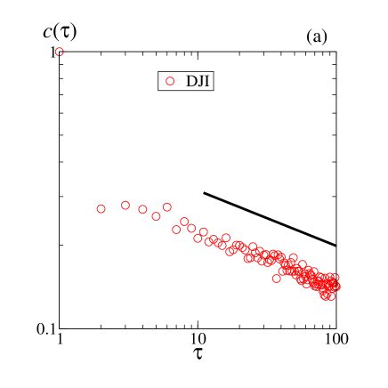
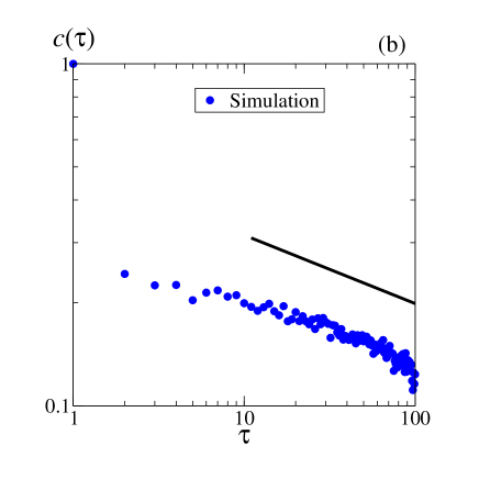
Figure  2.: (a) Log-log plot of the empirical volatility autocorrelation at time separation $\tau$ (in days), $c(\tau)\equiv\frac{\sum_{t=0}^{t_{max}}|r(t,1)||r(t+\tau,1)|-\sum_{t=0}^{t_{max}}|r(t,1)|\sum_{t=0}^{t_{max}}|r(t+\tau,1)|/t_{max}}{\sum_{t=0}^{t_{max}}|r(t,1)|^{2}-[\sum_{t=0}^{t_{max}}|r(t,1)|]^{2}/t_{max}},$ where $t_{max}+\tau-1$ is the total length of the time series. The data refer to the DJI index and $t_{max}+\tau-1$ is about $26000$ days. The continuous line has slope $\simeq-0.2$, the exponent of the power-law decay. In (b) the empirical data have been replaced by data from the simulation of one history.

Indicating by $\tilde{p}_{2T}^{(2)}(k_{1},k_{2})$ the CF of the joint PDF $p_{2T}^{(2)}$, Eqs. (2-4) above read:

$$\tilde{p}_{2T}^{(2)}(k,k) = \tilde{g}(\sqrt{2T}\;k),$$ (6)

$$\tilde{p}_{2T}^{(2)}(k,0) = \tilde{g}(\sqrt{T}\;k),$$ (7)

$$\tilde{p}_{2T}^{(2)}(0,k) = \tilde{g}(\sqrt{T}\;k),$$ (8)

where $D=1/2$ has been already substituted. It is then immediate to realize that a possible solution is simply:

$$\tilde{p}_{2T}^{(2)}(k_{1},k_{2})=\tilde{g}\left(\sqrt{Tk_{1}^{2}+Tk_{2}^{2}}\right),$$ (9)

provided such a $\tilde{p}_{2T}^{(2)}$ is a characteristic function, i.e. its inverse-transform is a PDF in $(r_{1},r_{2})$. This is not of course the case for any $\tilde{g}$, but one can show that there is a large class of CF’s satisfying this requisite, as can be checked by numerics  [?], or established on the basis of rigorous theorems  [?]. The solution in Eq. (9) is of course not the unique possibility. However, it is strongly suggested, in first place, by the good consistency it demonstrates with the statistical data. When sampled over the whole history of the DJI index from $1900$ to $2005$, the histograms of the empirical conditional PDF’s of a return $r_{2}$ once a previous return of modulus $|r_{1}|$ has been realized, are very well reproduced by the analytical prediction based on Eq. (9) (Fig. 3). The analytical expression for $\tilde{p}_{2T}^{(2)}$, and thus of $p_{2T}(r_{2}||r_{1}|)$, is here obtained on the basis of a particular form of $\tilde{g}$  [?], whose parameters have been fixed by a preliminary fit of $g$ as illustrated in Fig. 1. In Fig. 3 we show the conditional PDF for a given $|r_{1}|$ at different values of $T$.

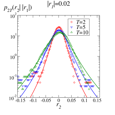
Figure  3.: Symbols are the empirical conditional PDF, $p_{2T}(r2||r_{1}|)$, of a return $r_{2}$ following $r_{1}$ with $|r_{1}|=0.02$. The continuous curves are obtained on the basis of Eq. (9), when $\tilde{g}$ results from the fit in Fig. 1

A further reason in favor of our solution is the fact that the recipe in Eq. (9) which constructs $\tilde{p}_{2T}^{(2)}$ through replacement of single argument dependence of $\tilde{g}$ by a spherically symmetric dependence in $(k_{1},k_{2})$, can be regarded as a rule of algebraic multiplication of $\tilde{g}(k_{1})$ by $\tilde{g}(k_{2})$. This type of multiplication, which is straightforwardly generalized to more than two factors, is commutative and associative, has as neutral element $\tilde{g}(0)=1$, and, most important, can be put at the basis of an extension of the central limit theorem for sums of strongly correlated variables  [?]. In this perspective Eq. (9) can be put in a form

$$\tilde{p}_{2T}^{(2)}(k_{1},k_{2})=\tilde{g}\left(\sqrt{T}k_{1}\right)\otimes\tilde{g}\left(\sqrt{T}k_{2}\right),$$ (10)

where the symbol $\otimes$ represents the non-standard multiplication  [?]. The $\otimes$ multiplication reduces to the standard one for Gaussian $g$’s  [?,?], and in this case Eq. (10) gives $\tilde{p}_{2T}^{(2)}(k_{1},k_{2})=\tilde{g}\left(\sqrt{T}k_{1}\right)\;\tilde{g}\left(\sqrt{T}k_{2}\right)$, consistently with Eq. (5).

3. Non-stationary stochastic model of index evolution

We already mentioned that the above solution in Eq. (9) can be generalized to the case of more than two successive intervals. Indeed, through our recipes we can construct a joint PDF for many returns. If, for example, we consider the CF corresponding to the joint PDF of $n$ successive daily returns, $p_{n1}^{(n)}$, this will be simply given by

$$\tilde{p}_{n1}^{(n)}(k_{1},k_{2},\ldots,k_{n}) = \tilde{g}(k_{1})\otimes\tilde{g}(k_{2})\otimes\cdots\otimes\tilde{g}(k_{n})$$ (11)

$$= \tilde{g}\left(\sqrt{k_{1}^{2}+k_{2}^{2}+\cdots+k_{n}^{2}}\right).$$ (12)

The joint PDF’s for various $n$ define a non-Markovian, self-similar stochastic process thanks to the algebraic properties of the $\otimes$ multiplication. It would be tempting to regard this process as the one which directly generated the history of the index to which $\tilde{g}$ pertains. Indeed, a nice property one can deduce for it is that for such a process returns would be stationary. So, the ensemble PDF for returns in the process could be directly sampled by the sliding interval procedure yielding the empirical $p_{T}$. Another nice property is that the process would be a martingale  [?], i.e. the conditional expectation of the future return is always zero, independent of the conditioning history. This is embodied in the construction of the $\tilde{p}_{n1}^{(n)}$, which are even in the their dependence on each of the $k_{i}$’s. However, there are clear indications that this simple scenario would be oversimplified, and that PDF’s like $p_{n1}^{(n)}$ cannot directly describe the postulated stochastic process potentially able to generate a whole ensemble of alternative histories.

The reasons why such a process with stationary increments would not be acceptable are two. In first place, for such a process the autocorrelation function of the absolute value of daily returns would not decrease with time, but rather be a constant, in disagreement with the empirical observation of a power law decay ( Fig. 2a)  [?]. Furthermore, one has to consider that the construction of $p_{n1}^{(n)}$ assumes a strict simple-scaling form for $p_{T}$. We know that this simple-scaling is well obeyed by this PDF only if we restrict ourselves to consider its lowest moments, i.e. $\langle|r|^{q}\rangle_{p_{T}}$ with $q\lesssim 3$, like we did in our argument leading to $D=1/2$. In fact multiscaling-like effects are observed in the scaling of higher moments  [?,?]. These effects mean that the $q$-th moment of $p_{T}$ scales as $T^{D(q)}$, with $D(q)<q/2$ for $q\gtrsim 3$, and would not be taken into account by the stochastic model.

A way out of the above difficulties is found if one considers that the very assumption of stationary increments for the process underlying index evolution is, a priori, not justified. Stationarity is often assumed on the basis of the fact that $p_{T}$ is stationary by construction. However, there is no compelling reason to do this and to identify $p_{T}$ with the PDF of the returns of the underlying process. The recent literature even reports indications that the stochastic processes driving exchange rates could be characterized by time-inhomogeneities in the returns  [?]. Within our scheme it is easy to embody the possibility of non-stationary returns in the ensemble generating process. The key is found going back to our arguments leading to the conclusion that $D=1/2$ for the empirical $p_{T}$. For the postulated non-stationary process driving the index, the ensemble PDF for returns like $r_{t,T}$ should be a function of both $t$ and $T$, which we indicate here by $P_{t,T}(r)$. Likewise, the joint PDF of the process corresponding to $p_{2T}^{(2)}$ can be indicated by $P_{t,2T}^{(2)}(r_{1},r_{2})$. Let us now consider the equations applying to these ensemble PDF’s and corresponding to Eqs. (3) and (4) for the empirical PDF’s. With $t=0$ for simplicity, one gets:

$$P_{0,T}(r_{1}) = \int dr_{2}P_{0,2T}^{(2)}(r_{1},r_{2}),$$ (13)

$$P_{T,T}(r_{2}) = \int dr_{1}P_{0,2T}^{(2)}(r_{1},r_{2}).$$ (14)

Eq. (2) is simply rewritten as

$$P_{0,2T}(r)=\int dr_{1}dr_{2}\;P_{0,2T}^{(2)}(r_{1},r_{2})\;\delta(r-r_{1}-r_{2}).$$ (15)

Suppose further that a simple-scaling form is valid for $P_{0,T}$, i. e.

$$P_{0,T}=\frac{1}{T^{D_{e}}}g_{e}\left(\frac{r}{T^{D_{e}}}\right),$$ (16)

with an ensemble scaling function $g_{e}$ and an ensemble dimension $D_{e}$. Consider now the ensemble average $\langle(r_{1}+r_{2})^{2}\rangle_{P_{0,2T}^{(2)}}$ in the light of Eqs. (13-16) and of $\langle r_{1}r_{2}\rangle_{P_{0,2T}^{(2)}}=0$. If we want to recast the r.h.s. of Eq (14) in the form of $P_{0,T^{\prime}}$, we realize that we must put $T^{\prime}=aT$, with $a=(2^{2D_{e}}-1)^{1/2D_{e}}$, in order to be consistent with the scaling assumed for $P_{0,T}$. If $D_{e}\neq 1/2$, there is an inhomogeneity in the process, measured by this rescaling $a$, which reveals an asymmetry between the first and the second $T$-interval considered. In other words, $a\neq 1$ signals a preferential direction of time: the evolution of the index in the second interval occurs with width rescaled with respect to that of the previous one. This effect is consistent with causality and the rescaling $T^{\prime}=aT$ is analogous to the rescaling of the block size $N$ which one would have when constructing marginal PDF’s for $M_{1}$ or $M_{2}$ in the magnetic RG. Of course, in that case, there would not be causality, and the rescaling would apply symmetrically to both PDF’s as a consequence of the correlations.

This argument already shows that our formalism leaves room for the construction of stochastic processes which are more general than that the one introduced in Eqs. (11-12). One has to follow steps similar to those which led us to construct the solution for $\tilde{p}_{2T}^{(2)}$ in terms of $\tilde{g}$, taking into account the presence of $a\neq 1$. For the CF of $P_{0,2T}^{(2)}$, for example, we get now $\tilde{P}_{0,2T}^{(2)}(k_{1},k_{2})=\tilde{g}_{e}\left(T^{D_{e}}k_{1}\right)\otimes\tilde{g}_{e}\left((aT)^{D_{e}}k_{2}\right)$. Similarly, for a sequence of $n$ daily returns, we can write:

$$\tilde{P}_{0,n1}^{(n)}(k_{1},k_{2},\ldots,k_{n})=\tilde{g}_{e}\left(a_{1}^{D_{e}}k_{1}\right)\otimes\tilde{g}_{e}\left(a_{2}^{D_{e}}k_{2}\right)\otimes\cdots\otimes g_{e}\left(a_{n}^{D_{e}}k_{n}\right),$$ (17)

where $a_{i}\equiv\left[i^{2D_{e}}-(i-1)^{2D_{e}}\right]^{1/2D_{e}}$; $i=1,2,\dots n$. These last CF’s again fully characterize a stochastic process, which is now non-stationary. The process is consistent with the simple-scaling of $P_{0,T}$, but now $P_{t,T}$ satisfies a more general, inhomogeneous form of scaling:

$$P_{t,T}(r)=\frac{1}{\sqrt{(t+T)^{2D_{e}}-t^{2D_{e}}}}\;\;g_{e}\left(\frac{r}{\sqrt{(t+T)^{2D_{e}}-t^{2D_{e}}}}\right).$$ (18)

On the basis of this last equation, one can try to analyze how the effective scaling dimension for $T$ of the order of the month varies as a function of $t$. This is illustrated in Fig. 4 for a value of $D_{e}=0.24$, which, as discussed below, is directly relevant for the application to the DJI index. One sees that, after a rather fast increase at short $t$, this effective dimension $D_{eff}$ approaches the value $1/2$, which is the asymptotic limit. Thus, if one would sample with sliding interval method a return PDF $p_{T}$ along a sufficiently long single history of the process consistent with Eq. (18), this PDF would show a scaling with $D\simeq 1/2$ for $T$ of the order of the month. At the same time, the initial deviation from $1/2$ of the effective dimension shown in Fig. 4 suggests that this $p_{T}$ could manifest multiscaling-like features.

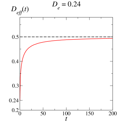
Figure  4.: Effective dimension $D_{eff}$ for $1\lesssim T\lesssim 40$ deduced from Eq. (18). This $D_{eff}$ is obtained from the behavior of the moments of $P_{t,T}$ as a function of $T$ in this range.

The problem arises now of postulating some concrete mechanism through which inhomogeneity can act in generating an index history. It is natural to assume that the inhomogeneity crosses over to homogeneity when $t$ exceeds some cut-off $t_{c}$. This cut-off time could be of the order of the autocorrelation time of volatility, i.e. several hundreds of days. Of course, $t_{c}$ should be regarded as a statistical average of the duration of many random intervals within which the process is described by a $P_{0,n1}^{(n)}$ corresponding to Eq. (17). At the junctions between these intervals, which can be imagined to coincide with relevant external events influencing the market, one could assume that the progression of the coefficients $a_{i}$ is suddenly interrupted and restarted, either from the beginning ($a_{i+1}=a_{1}$), or from a randomly chosen stage ($a_{i+1}=a_{k}$, with $k\neq 1$).

4. Simulation of the model and results for the DJI index

The knowledge of $P_{n1}^{(n)}$ allows to implement an autoregressive strategy for the simulation of the process. Autoregressive methods are used extensively in finance, e.g. for the implementation of ARCH or GARCH processes  [?,?]. Suppose we consider $P_{n1}^{(n)}$, with, e.g., $n=100$. If we give as input the first $99$ returns, the joint PDF can be used in order to define the conditional PDF of the return in the hundredth day. Once this return is extracted consistently, one can use the returns from the second to the hundredth day included in order to extract in a similar way the return of the $101$-th day, and so on. Without entering into the details of how this is practically implemented  [?], here we just review the results one can obtain.

By expressing $P_{n1}^{(n)}$ in terms of $\tilde{g}_{e}$, whose expansion around $k=0$ is directly linked to that of the empirical $\tilde{g}$  [?], we generate single histories supposed to imitate the one at our disposal with over one century of DJI index daily closures. In all cases we fix $t_{0}=500$ on average for the inhomogeneity updating and $n=100$ for the auto-regressive scheme. Once a single history is generated, we act on it, by sliding interval sampling techniques, exactly in the same way one does on the true historical series. Upon varying $D_{e}$, which is the crucial parameter in the simulation, we search for the most realistic behavior of the empirical volatility autocorrelation function in the range from few to about hundred days. Remarkably enough, for $D_{e}<1/2$ the obtained autocorrelation functions behave as decaying power laws in this range, and the exponent becomes very close to the empirical one ($\beta\simeq 0.2$) for $D_{e}\simeq 0.24$, (see Fig. 2b and  [?]). At the same time, we can try to optimize $D_{e}$ by requesting a realistic agreement between the multiscaling features of the simulated $p_{T}$ and those of the empirical one. It is remarkable that the optimal $D_{e}$ according to this second criterion is very close again to $0.24$  [?]. This is a further indication that the model is coherent and catches the essential statistical features of a long index history.

A very important test for the proposed model concerns the scaling of the empirical $p_{T}$ itself. A crucial limitation of simulation methods like ARCH and GARCH is that they generate histories for which it is not guaranteed that the sampled $p_{T}$ satisfies scaling. This is in fact regarded as a major open problem of these approaches [?]. In Fig. 5 we report the scaling collapse of $p_{T}$ as obtained by one of the histories generated by our simulation. The collapse is clearly of the same quality as that reported in Fig 1; moreover, the scaling function and the exponent emerging from the collapse are very consistent with those valid for the historical data.

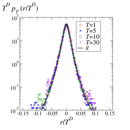
Figure  5.: Scaling collapse of the $p_{T}$ sampled from a single simulated history.

The general agreement between the stylized features of the simulated histories and those of the the true history  [?], suggest that our model based on inhomogeneous scaling and market efficiency catches the robust features of the stochastic component of index evolution.

5. Conclusions

The results reviewed in this report show the importance of scaling in building up a model of stochastic index evolution in finance. In the construction of the model this symmetry enters as a very crucial tool, in the sense that, combined with other constraints, it leads to fix very plausible and consistent rules of probabilistic evolution. In view of the success of the model, the skepticism on the practical relevance of scaling mentioned in the introduction, should be attenuated. A crucial factor which helps in converting scaling into a powerful predictive tool here, is that we regard it in a perspective which has roots in the RG approach to criticality. This allows even to establish novel paradigms, like the one represented by the inhomogeneous scaling in Eq. (18). More generally, the strategy followed here tries to profit of the lessons learned from decades of work in complex systems. As clearly stated in Ref.  [?], the issue of financial market modeling should be addressed by first trying to focus on the universal phenomenological features, and on the basic symmetries, rather then privileging analytical tractability.

We believe that the approach presented here could have more general applicability. There are many natural phenomena characterized by anomalous scaling, for which part of the features of the model discussed here, or of the arguments leading to it, could reveal worth considering. These problems belong in general to the fields of multidisciplinary applications of statistical mechanics.

REFERENCES

- [1] M. Gallegati, S. Keen, T. Lux and Paul Ormerod, Physica A 370, 1 (2006).
- [2] B. LeBaron, Nature 408, 290 (2000).
- [3] H.E. Stanley, L.A.N. Amaral, S.V. Buldyrev, P. Gopikrishnan, V. Plerou and M.A. Salinger, Proc. Natl. Acad. Sci 99, 2561 (2002).
- [4] F. Baldovin and A.L. Stella, Proc. Natl. Acad. Sci 104, 19741 (2007).
- [5] R. Cont, Quant. Finance 1, 223 (2001); in Fractals in Engineering, eds. E. Lutton and J. Levy Véhel, Springer-Verlag, New York (2005).
- [6] J.-P. Bouchaud and M. Potters, Theory of Financial Risks, Cambridge University Press, Cambridge, UK (2000).
- [7] R.N. Mantegna and H.E. Stanley An Introduction to Econophysics, Cambridge University Press, Cambridge, UK, (2000).
- [8] K. Yamasaki, L. Muchnik, S. Havlin, A. Bunde, and H.E. Stanley, Proc. Natl. Acad. Sci. USA 102, 9424 (2005).
- [9] T. Lux, in Power Laws in the Social Sciences, eds. C. Cioffi-Revilla, Cambridge University Press, Cambridge, UK, (in press).
- [10] L. Bachelier, Ann. Sci. Ecole Norm. Sup. 17, 21 (1900).
- [11] G. Jona-Lasinio Phys. Rep. 352, 439 (2001).
- [12] L.P. Kadanoff, Statistical Physics, Statics, Dynamics and Renormalization, World Scientific, Singapore (2005).
- [13] F. Baldovin and A.L. Stella, Phys. Rev. E 75, 020101(R) (2007).
- [14] T. Di Matteo, T. Aste and M.M. Dacorogna, J. Bank. & Fin. 29, 827 (2005).
- [15] M.P. Nightingale, Physica A 83, 561 (1976); see also T.W. Burkhardt and J.M.J. van Leeuwen eds., Real-Space Renormalization, Springer-Verlag, Berlin Heidelberg (1982).
- [16] See, e.g., B.V. Gnedenko and A.N. Kolmogorov, Limit Distributions for Sums of Independent Random Variables, Addison Wesley, Reading, MA (1954).
- [17] F. Baldovin and A.L. Stella, to be published (2008).
- [18] I.M. Sokolov, A.V. Chechkin and J Klafter, Physica A 336, 245 (2004).
- [19] W. Feller, An Introduction to Probability Theory and Its Applications, Vol 2, John Wiley & Sons (2nd edition 1971);
- [20] K.E. Bassler, J.L. McCauley and G.H. Gunaratne, Proc. Natl. Acad. Sci 104, 17287 (2007).
- [21] R. Engle, Journal of Money, Credit and Banking 15, 286 (1983).
- [22] T. Bollerslev, Journal of Econometrics 31, 307 (1986).
- [23] N. Goldenfeld and L.P. Kadanoff, Science 284, 87 (1999).