On the Truncated Pareto Distribution with applications

Abstract

The Pareto probability distribution is widely applied in different fields such us finance, physics , hydrology , geology and astronomy. This note deals with an application of the Pareto distribution to astrophysics and more precisely to the statistical analysis of mass of stars and of diameters of asteroids. In particular a comparison between the usual Pareto distribution and its truncated version is presented. Finally a possible physical mechanism that produces Pareto tails for the distribution of the masses of stars is suggested.

95.75.-z Observation and data reduction techniques; computer modelling and simulation ; 96.30.Ys Asteroids, meteoroids 97.10.Xq Stars: Luminosity and mass functions

1 Introduction

The Pareto distribution [1, 2]. is a simple model for nonnegative data with a power law probability tail. In many practical applications, it is natural to consider an upper bound that truncates the tail [3, 4, 5]; the truncated Pareto distribution has a wide range of applications in several fields in data analysis [5] [6].

Power law distributions are often found in astrophysics: for instance in the range $1\mathcal{M}_{\hbox{$\odot$}}~{}<~{}\mathcal{M}<10\mathcal{M}_{\hbox{$\odot$}}$, the mass of the stars (MAIN SEQUENCE V), when expressed in terms of the solar mass $\mathcal{M}_{\hbox{$\odot$}}$, scales as $\psi({\mathcal{M}})\propto{\mathcal{M}}^{-\alpha}$ with $\alpha$= 2.35, see [7] or $\alpha$= 2.3 as suggested by a recent evaluation , see [8]. Other examples are the intensity of non thermal emission from supernova remnant and extra-galactic radio-sources that scales as $\nu^{-\alpha}$, with numerical values of $\alpha$ ranging between 0.5 and 1, the observed differential spectrum of cosmic rays proportional to $E^{-2.75}$ in the interval $10^{10}~{}eV-5.0~{}10^{15}~{}eV$ [9, 10], the gamma ray bursts luminosity function that scales as $L^{-2}$, [11, 12]. Of course the Pareto distribution is not the only one to exhibit power law tail, this behaviour being common to different distributions (e.g. the lognormal distribution); however Pareto distributions are specially attractive for their simple analytical form.

In this paper we present in Section 2 a comparison between the Pareto and the truncated Pareto distributions. In Section 3 the theoretical results are applied to distribution of astrophysical data, namely the mass of stars and the radius of asteroids. A physical mechanism that produces a Pareto type distribution for the masses is presented in Section 4

2 Preliminaries

Let $X$ be a random variable taking values $x$ in the interval $[a,\infty]$, $a>0$. The probability density function (in the following pdf) named Pareto is defined by [2]

$$f(x;a,c)={ca^{c}}{x^{-(c+1)}}\quad,$$ (1)

$c~{}>0$, and the Pareto distribution functions is $F(x:a,c)=1-a^{c}x^{-c}$

An upper truncated Pareto random variable is defined in the interval $[a,b]$ and the corresponding pdf is

$$f_{T}(x;a,b,c)=\frac{ca^{c}x^{-(c+1)}}{1-\left(\frac{a}{b}\right)^{c}}\quad,$$ (2)

[5] and the truncated Pareto distribution function is

$$F_{T}(x;a,b,c)=\frac{1-(\frac{a}{x})^{c}}{1-(\frac{a}{b})^{c}}\quad.$$ (3)

Momenta of the truncated distributions exist for all $c>0$. For instance, the mean of $f_{T}(x;a,b,c)$ is, for $c\neq 1$ and $c=1$, respectively,

$$<x>=\frac{ca}{c-1}\frac{1-(\frac{a}{b})^{c-1}}{1-(\frac{a}{b})^{c}},\quad<x>=\frac{ca^{c}}{1-\left(\frac{a}{b}\right)^{c}}\ln\frac{b}{a}$$ (4)

Similarly, if $c\neq 2$, the variance is given by

$$\sigma^{2}=\frac{ca^{2}}{(c-2)}\frac{1-\left(\frac{a}{b}\right)^{c-2}}{1-\left(\frac{a}{b}\right)^{c}}-<x>^{2},$$ (5)

whereas for $c=2$

$$\frac{ca^{c}}{1-\left(\frac{a}{b}\right)^{c}}\ln\frac{b}{a}-<x>^{2}.$$ (6)

In general the $n-th$ central moment is

$$\int_{a}^{b}(x-<x>)^{n}f_{T}(x)dx=$$

$$\left(-{\it<x>}\right)^{n}{a}^{-c}{~{}_{2}F_{1}(-c,-n;\,1-c;\,{\frac{a}{{\it<x>}}})}\left(\left({a}^{c}\right)^{-1}-\left({b}^{c}\right)^{-1}\right)^{-1}$$

$$-\left(-{\it<x>}\right)^{n}{b}^{-c}{~{}_{2}F_{1}(-c,-n;\,1-c;\,{\frac{b}{{\it<x>}}})}\left(\left({a}^{c}\right)^{-1}-\left({b}^{c}\right)^{-1}\right)^{-1}$$ (7)

where ${~{}_{2}F_{1}(a,b;\,c;\,z)}$ is a regularized hypergeometric function, see [13, 14, 15]. An analogous formula based on some of the properties of the incomplete beta function, see [16] and [17] , can be found in [18].

Parameters of the truncated Pareto pdf from empirical data can be obtained via the maximum likelihood method; explicit formulas for maximum likelihood estimators (MLE) are given in [3], and for the more general case in [5], whose results we report here for completeness.

Consider a random sample ${\mathcal{X}}=x_{1},x_{2},\dots,x_{n}$ and let $x_{(1)}\geq x_{(2)}\geq\dots\geq x_{(n)}$ denote their order statistics so that $x_{(1)}=\max(x_{1},x_{2},\dots,x_{n})$, $x_{(n)}=\min(x_{1},x_{2},\dots,x_{n})$.

The MLE of the parameters $a$ and $b$ are

$${\tilde{a}}=x_{(n)},\qquad{\tilde{b}}=x_{(1)},$$ (8)

respectively, and $\tilde{c}$ is the solution of the equation

$$\frac{n}{{\tilde{c}}}+\frac{n(\frac{x_{(n)}}{x_{(1)}})^{\tilde{c}}\ln(\frac{x_{(n)}}{x_{(1)}})}{1-(\frac{x_{(n)}}{x_{(1)}})^{\tilde{c}}}-\sum_{i=1}^{n}[\ln x_{i}-\ln x_{(n)}]=0,$$ (9)

[5].

There exists a simple test to see whether a Pareto model is appropriate [5]: the null hypothesis $H_{0}:\nu=\infty$ is rejected if and only if $x_{(1)}<[nC/(-\ln q)]^{1/c}$, $0<q<1$, where $C=a^{c}$. The approximate $p$-value of this test is given by $p=\exp\left\{-nCx^{-c}_{(1)}\right\}$, and a small value of $p$ indicates that the Pareto model is not a good fit; of course this is not enough per se to demonstrate the goodness of a truncated Pareto distribution.

Given a set of data is often difficult to decide if they agree more closely with $f$ or $f_{T}$, in that, in the interval $[a,b]$, they differ only or a multiplicative factor $1-(a/b)^{c}$, that if the interval $[a,b]$ is not too small approaches $1$ even for relatively small values of $c$. For this reason, rather than $f$ and $f_{T}$, the distributions $P(X>x)$ and $P(X>x)$ are used, often called survival functions, that are given respectively by

$$P(X>x)=S(x)=1-F(x;a,c)=a^{c}x^{-c}$$ (10)

and

$$P_{T}(X>x)=S_{T}(x)=1-F_{T}(x;a,b,c)=\frac{ca^{c}\left(x^{-c}-b^{-c}\right)}{1-\left(\frac{a}{b}\right)^{c}}.$$ (11)

Probabilities $P$ and $P_{T}$ have qualitatively different trends that are better observed in a log-log plot. In this case $P$ is obviously represented by a straight line, whereas $P_{T}$ exhibits also a almost linear trend with a sharp drop when $x$ tends to $b$. To illustrate this point we have generated a set of $n=10000$ random points drawn from a truncated Pareto distribution, via the formula

$$X:a,b,c\sim a\left(1-R({1-(\frac{a}{b})^{c})}\right)^{-\frac{1}{c}}\quad,$$ (12)

where $R$ is the unit rectangular variate, and we have fitted them with $S$ and $S_{T}$ respectively, see Figure 1.

Figure 1: log–log plot of the survival function: 10000 random data (empty circles), generated with Eq. (12), survival function of the truncated Pareto distribution (full line) and survival function of the Pareto distribution (dotted line).

3 Applications

3.1 Mass of stars

The sample of star’s masses has been obtained from the Hipparcos data as a function of the absolute magnitude and (B-V) [19]. Results of the fitting with $P$ and $P_{T}$ are presented in Table 1 where $a,b,c$ and $n$, the number of sample elements, are reported and in Figure 2 that shows the data with the fit.

Table 1: Coefficients of mass distribution of the stars in the first 10 pc, of a complete sample (MAIN SEQUENCE V). The parameter $c$ is derived through MLE and p=0.032.

a [$\mathcal{M}_{\hbox{$\odot$}}$]	b [$\mathcal{M}_{\hbox{$\odot$}}$]	c	n	$P(X>x)$
0.53	3.44	1.45	52	Truncated Pareto
0.53	$\infty$	1.77	52	Pareto

Figure 2: log–log plot of the survival function of the mass distribution of the stars: data (empty circles), survival function of the truncated Pareto pdf (full line) and survival function of the Pareto pdf (dotted line). A complete sample (MAIN SEQUENCE V) is considered with parameters as in Table 1.

In this case in the range $3.44\mathcal{M}_{\hbox{$\odot$}}~{}>~{}\mathcal{M}\geq 0.53\mathcal{M}_{\hbox{$\odot$}}$, see Table 1 , the coefficient $\alpha=c+1$ =2.45 is in agreement with modern estimates [8]. In this case, the power of the Pareto test results to be $p=0.032$, indicating that the Pareto distribution is not a good fit, as can also be seen from Figure 2 .

Table 2 therefore reports the $\chi^{2}$ of the fit of the stars when the Pareto and the truncated Pareto, respectively.

Table 2: $\chi^{2}$ of different distributions when the number of bins is 5 for the stars in the first 10 $pc$ .

Distribution	$\chi^{2}$
Pareto	7.1
Truncated Pareto	5.26

3.2 Distribution of asteroids size

Suppose that not just masses of stars but also those of other astrophysical objects have a power law tail, then is not difficult to prove that also their linear dimension, radii or diameters, must follows a power law. We have tested this hypothesis by considering diameters of different families of asteroids, namely, Koronis , Eos and Themis.

In the following The sample parameter of the families are reported in Table 3,Table 4 and Table 5 , whereas Figure 3, Figure 4, Figure 5 report the graphical display of data and the fitting distributions.

Table 3: Coefficients of diameter distribution of the Koronis family . The parameter $c$ is derived through MLE and p=0.033 .

a [km]	b [km]	c	n	$P(X>x)$
25.1	44.3	3.77	29	truncated  Pareto
25.1	$\infty$	5.04	29	Pareto

Table 4: Coefficients of diameter distribution of the Eos family . The parameter $c$ is derived through MLE and p=0.681 .

a [km]	b [km]	c	n	$P(X>x)$
30.1	110	3.80	53	truncated  Pareto
30.1	$\infty$	3.94	53	Pareto

Table 5: Coefficients of diameter distribution of the Themis family . The parameter $c$ is derived through MLE and p=0.67 .

a [km]	b [km]	c	n	$P(X>x)$
35.3	249	2.5	53	truncated  Pareto
35.3	$\infty$	2.6	53	Pareto

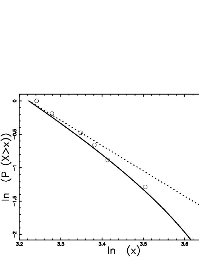
Figure 3: ln–ln plot of the survival function of diameter distribution of the Koronis Family: data (empty circles), survival function of the truncated Pareto pdf (full line) and survival function of the Pareto pdf (dotted line). A complete sample is considered with parameters as in Table 3.

Figure 4: ln–ln plot of the survival function of diameter distribution of the Eos Family: data (empty circles), survival function of the truncated Pareto pdf (full line) and survival function of the Pareto pdf (dotted line). A complete sample is considered with parameters as in Table 4.

Figure 5: ln–ln plot of the survival function of diameter distribution of the Themis Family: data (empty circles), survival function of the truncated Pareto pdf (full line) and survival function of the Pareto pdf (dotted line). A complete sample is considered with parameters as in Table 5.

In case of the Koronis family $P_{T}$ fits the data better than $P$ and indeed $p=0.039$ is correspondingly small, whereas for the Eos family, $P$ performs slightly better than $P_{T}$ (p=0.68), and the estimated of $c$ are very closed in both cases. Finally in the third case, the Themis family, the two distributions are the same, due to the fact that the ratio $a/b=0.14$ is small.

4 Generating Pareto tails

As a simple example of how a distribution with power can be generated, consider the growth of a primeval nebula via accretion, that is the process by which nebulae “capture” mass. We start by considering an uniform pdf for the initial mass of $N$ primeval nebulae, $m$, in a range $m_{min}<m\leq m_{max}$ . At each interaction the $i$-th nebula has a probability $\lambda_{i}$ to increase its mass $m_{i}$ that is given by

$$\lambda_{i}=(1-\exp(-akm_{i})),$$ (13)

where $ak$ is a parameter of the simulation; thus more “massive” nebulae are more likely to grow, via accretion. The quantity of which the primeval nebula can grow varies with time, to take into account that the total mass available is limited,

$$\delta m(t)=\delta m(0)\exp(-t/\tau)\quad,$$ (14)

where $\delta m(0)$ represents the maximum mass of exchange and $\tau$ the scaling time of the phenomena. The simulation proceeds as follows: a number $r$, is randomly chosen in the interval $[0,1]$ for each nebula, and, if $r<\lambda_{i}$, the mass $m_{i}$ is increased by $\delta m(t)$, where $t$ denotes the iteration of the process. The process proceed in parallel : at each temporal iteration all the primeval nebulae are considered.

Results of the simulations have been fitted with both Pareto survival distributions. see Figure 6

Due to a photometric effect [19] the sample of observed stars is complete only for $m\geq 0.5\mathcal{M}_{\hbox{$\odot$}}$. We therefore have set the lower boundary of the masses to $0.5\mathcal{M}_{\hbox{$\odot$}}$, and the resulting subset has been fitted with the Pareto and truncated Pareto survival distributions, Figure 6. It should be noted that the results of the simulation give $c=1.36$, that is $\alpha=2.36$ in agreement with the experimental estimate.

Figure 6: log–log plot of the survival function of the mass distribution for the primeval nebula when $m\geq 0.5\mathcal{M}_{\hbox{$\odot$}}$ are considered. The truncated Pareto parameters are $c$=1.36 and p=0.0058 .

5 Conclusions

Results of the analysis presented here show that the truncated Pareto distribution provides a good fit for the distribution and performs better than the usual Pareto distribution. When the asteroid diameters are considered the situation is not so clear in that it depends on the family one considers. It is also clear the there can be cases, such as with the Themis family, in which the ratio between the minimum and the maximum value of the sample is so small that there no real difference between the two distributions. Finally we have shown that Pareto distributions can result from a simple growth process, in which the increase of the state variable (here mass) depends on the values taken in the previous state; furthermore results of the simulations agree well with the experimental data.

As remarked earlier distributions are not the only statistics with a power law tail; also in astrophysics alternatives have been proposed for the statistics of asteroid diameters (e.g. [20]). However Pareto distributions are particularly simple; for instance note that they have just a free parameter $c$, the others $a$ and $b$, being determined by the minimum and maximum values of the sample, respectively.

References

- [1] V. Pareto, Cours d’ economie politique, Rouge, Lausanne, 1896.
- [2] M. Evans, N. Hastings, P. B., Peacock,B. , Statistical Distributions - third edition, John Wiley & Sons Inc, New York, 2000.
- [3] A. Cohen, B. Whitten, Parameter Estimation in reliability and Life Span Models, Marcel Dekker, New York, 1988.
- [4] D. Devoto, S. Martínez, : Truncated pareto law and oresize distribution of ground rocks, Mathematical Geology , Vol. 30 (6) , (1998),pp. 661 – 673.
- [5] I. Aban, M. Meerschaert, A. Panorska, : Parameter estimation for the truncated pareto distribution , Journal of the American Statistical Association , Vol. 101 , (2006),pp. 270–277.
- [6] K. Rehfeldt, J. M. Boggs, L. W. Gelhar, : Field study of dispersion in a heterogeneous aquifer. 3: Geostatistical analysis of hydraulic conductivity, Water Resour. Res. , Vol. 28 , (1992),pp. 3309–3324.
- [7] E. E. Salpeter, : The Luminosity Function and Stellar Evolution., ApJ , Vol. 121 , (1955),pp. 161–+.
- [8] P. Kroupa, : On the variation of the initial mass function, MNRAS , Vol. 322 , (2001),pp. 231–246.
- [9] K. R. Lang, Astrophysical formulae, Springer, New York, 1999.
- [10] R. Schlickeiser, Cosmic ray astrophysics, Springer, Berlin, 2002.
- [11] E. M. Rossi, : Structure of gamma ray burst jets, Nuovo Cimento C Geophysics Space Physics C , Vol. 28 , (2005),pp. 387–+.
- [12] J. S. Bloom, D. A. Frail, R. Sari, : The Prompt Energy Release of Gamma-Ray Bursts using a Cosmological k-Correction, AJ , Vol. 121 , (2001),pp. 2879–2888.
- [13] M. Abramowitz, I. A. Stegun, Handbook of mathematical functions with formulas, graphs, and mathematical tables, Dover, New York, 1965.
- [14] D. von Seggern, CRC Standard Curves and Surfaces, CRC, New York, 1992.
- [15] W. J. Thompson, Atlas for computing mathematical functions, Wiley-Interscience, New York, 1997.
- [16] I. Gradshteyn, I. Ryzhik , Table of Integrals, Series, and Products, Academic Press, San Diego, 2000.
- [17] A. Prudnikov, O. Brychkov , Y. Marichev , Integrals and Series, Gordon and Breach Science Publishers, Amsterdam, 1986.
- [18] M. Masoom Ali, S. Nadarajah, : A truncated pareto distribution, Computer Communications , Vol. 30 , (2006),pp. 1–4.
- [19] L. Zaninetti, : The Initial Mass Function as given by the fragmentation, Astronomische Nachrichten , Vol. 326 , (2005),pp. 754–759.
- [20] L. Zaninetti, A. Cellino, V. Zappala, : On the fractal dimension of the families of the asteroids., A&A , Vol. 294 , (1995),pp. 270–273.