A Discrete Representation of Einstein’s Geometric Theory of Gravitation: The Fundamental Role of Dual Tessellations in Regge Calculus

In 1961 Tullio Regge provided us with a beautiful lattice representation of Einstein’s geometric theory of gravity. This Regge Calculus (RC) is strikingly different from the more usual finite difference and finite element discretizations of gravity. In RC the fundamental principles of General Relativity are applied directly to a tessellated spacetime geometry. In this manuscript, and in the spirit of this conference, we reexamine the foundations of RC and emphasize the central role that the Voronoi and Delaunay lattices play in this discrete theory. In particular we describe, for the first time, a geometric construction of the scalar curvature invariant at a vertex. This derivation makes use of a new fundamental lattice cell built from elements inherited from both the simplicial (Delaunay) spacetime and its circumcentric dual (Voronoi) lattice. The orthogonality properties between these two lattices yield an expression for the vertex-based scalar curvature which is strikingly similar to the corresponding and more familiar hinge-based expression in RC (deficit angle per unit Voronoi dual area). In particular, we show that the scalar curvature is simply a vertex-based weighted average of deficits per weighted average of dual areas. What is most striking to us is how naturally spacetime is represented by Voronoi and Delaunay structures and that the laws of gravity appear to be encoded locally on the lattice spacetime with less complexity than in the continuum, yet the continuum is recovered by convergence in mean. Perhaps these prominent features may enable us to transcend the details of any particular discrete model gravitation and yield clues to help us discover how we may begin to quantize this fundamental interaction.

1 Why Regge Calculus?

If nature is, at its very foundation, best expressed as a discrete theory – a finite representation based upon the elementary quantum phenomena, then how will such a corpuscular structure reveal itself by observation or measurement? If the quantum character of nature has taught us anything, it has taught us that (1) the observer and the observed are demonstrably coupled, and that (2) the basis of observation lay on the distinguishability between complementary observables. The currency of the quantum is information – information communicated from observer to observer in the form of quantum bits (qbits.) It is hard to imagine setting the stage for such a theory, and many have worked to do so. We believe that one small step can be made in this direction by examining a discrete representation of Einstein’s 1915 classical theory of gravitation – one of the purest geometric theories of nature we know. One may hope that by studying a discrete representation of gravitation, one may be able to glean some of the fundamental features of the discretization that may yield way points to true understanding of the basic building blocks of nature.

Fortunately, in 1961 Tullio Regge introduced a beautiful simplicial representation of Einstein’s geometric theory of gravitation R61 . It is referred to in the literature as Regge Calculus (RC). This approach represents the curved 4-dimensional spacetime geometry, which is so central to General Relativity (GR), as a discrete 4-dimensional simplicial lattice. The interior geometry of each simplex in this lattice is that of the flat spacetime geometry of Minkowski space. Since the beginnings of RC many researchers have successfully applied RC to many problems in both classical and quantum GR (references in TW92 ).

What is so striking to us is how naturally the concepts of the Voronoi and Delaunay lattices book appear in every facet of RC, and we think this representation applies to any discretization of spacetime. Perhaps this is not so surprising as witnessed by these proceedings of the vast applications the concepts of these lattices have throughout nature. We see them naturally appearing in nature from biological structures to anthropological applications, and from cosmology to the quantum and foams. It is the purpose of this paper to demonstrate concretely the necessary and natural role these Voronoi and Delaunay structures have in discrete models of gravity. CMS82 ; CMS84 ; H86 ; M86 ; M92 ; L82 That these two circumcentric lattices have encoded in them beautiful orthogonality properties, natural duality as well as a democratic way of assigning a unique and indisputable “territory” to every single event (atom, vertex, star, observer etc…) gives us hope as to their universality – hope that they can be used, in part, as an austere description of fundamental physics.

After briefly introducing some of the key features of Einstein’s theory of GR (Sec. 2) that we use in RC, we will describe how to understand the curvature of a lattice spacetime in in RC (Sec. 3). A detailed analysis of this lattice curvature, we show, yields a natural tiling of the lattice spacetime in terms of a new and fundamental 4-dimensional lattice cell – a hybridization of both the Voronoi lattice and the Delaunay lattice (Sec. 4). We demonstrate the usefulness of this new spacetime building block in RC by re-deriving the RC version of the Einstein-Hilbert action principle, and in the local construction of the Einstein tensor in RC. This coupling of the Voronoi and Delaunay lattices is further used to provide the first geometric construction of the scalar curvature invariant of which we are aware (Sec. 5-6). In particular, we show that the scalar curvature is simply a vertex-based weighted average of deficits per weighted average of dual areas. We provide (Sec. 7) an example of this vertex-based scalar curvature and discuss its convergence-in-mean to the continuum counterpart.

2 Gravitation and the Curvature of Spacetime

The geometric nature of the gravitational interaction is captured in Einstein’s theory of GR by a single equation MTW73 .

$$\underbrace{G_{\mu\nu}}_{\begin{array}[]{c}Curved\\ Spacetime\\ Geometry\end{array}}=8\pi\underbrace{T_{\mu\nu}}_{\begin{array}[]{c}Matter\\ and\\ Fields\end{array}}$$ (1)

Here the curvature of spacetime, as encapsulated by the ten-component Einstein tensor $G_{\mu\nu}$, acts on matter telling it how to curve, and in response these non-gravitational matter sources (the stress-energy tensor $T_{\mu\nu}$) react back on spacetime telling it how to curve. Central to this theory of gravity is the 4-dimensional curved spacetime geometry. This geometry is represented by a $4\times 4$ metric tensor $g_{\mu\nu}$, or by the edge lengths of a tessellated geometry as we will see below.

Central to Einstein’s theory is curvature and key to our description of RC in (Sec. 3) is the construction of the Riemann curvature tensor and the scalar curvature invariant on a Voronoi/Delaunay spacetime lattice. The components of the curvature tensor can be understood geometrically by either geodesic deviation or by the parallel transport of a vector around a closed loop. In RC is is most convenient to implement the latter. Here we illustrate curvature by a familiar example, the Gaussian curvature by way of parallel transport of a vector around a closed loop (Fig 1).

$$\mbox{Curvature}=K=\frac{\left(\begin{array}[]{c}\mbox{Angle Vector}\\ \mbox{Rotates}\end{array}\right)}{\left(\begin{array}[]{c}\mbox{Area}\\ \mbox{Circumnavigated}\end{array}\right)}=\frac{\frac{\pi}{2}}{\frac{1}{8}\left(4\pi R_{\oplus}^{2}\right)}=\frac{1}{R^{2}_{\oplus}}$$ (2)

Figure 1: The curvature of the Earth, idealized though it is as a sphere of radius $R_{\oplus}$, as revealed by parallel transport of a vector around a closed loop: We can demonstrate this equation by application to the 2-dimensional surface of the Earth. We show in this figure the clockwise circumnavigation of one quadrant of the northern hemisphere of the Earth. The starting point is the northward pointing vector on the equator, and three snapshots of this vector as it is parallel transported to the North Pole. The parallel transport of the vector is with respect to the geometry intrinsic to the surface of the sphere as there is no need whatsoever of relying on the embedding of the sphere in the Euclidean 3-dimensional geometry. That this vector is parallel transported parallel to itself is demonstrated that at every point on its northward journey up the longitudinal direction its always tangent to its path. Upon reaching the north pole, we take great care not to take the energy needed to rotate the vector even though our new path takes an abrupt turn to the right as we head southward down another longitude. In the beginning of this southward segment of our journey, at the North Pole, the vector is normal to this new longitudinal direction, and remains so because it is transported parallel to itself all the way back to the equator. At the equator the path takes another abrupt right angle turn toward the west. The vector which has never been rotated remains pointing eastward on the equator as it is parallel transported back along the equator to its starting position. As the vector returns to its starting point one can’t help but notice that it is rotated perpendicular to its original northward direction, although the vector was never rotated throughout its entire journey – a journey which swept out an area $1/8$ of the surface of the Earth. The reason for the net rotation is clear. The path circumnavigated contained a geometry of constant curvature. It is through this process of parallel transport that we can most clearly understand and analyze the curvature of a lattice spacetime geometry in RC.

In the 2-dimensional example of curvature shown above, only a single component of curvature is needed to completely characterize the curvature. There is only one tangent plane at each point on the surface that can be used to form a loop to circumnavigate. However in 4-dimensions there are many more orientations of areas to circumnavigate (Table 1). In addition to a scalar curvature, we actually need the structure of a tensor to characterize the curvature. This curvature is represented by the Riemann curvature tensor (3). Each of its components (twenty in the four dimensions of spacetime) are as easily described in the same fundamental way in which we obtained the curvature of the earth in Fig. 1 – by parallel transport of a vector about a vanishingly small closed loop.

$${\cal R}=\left(\begin{array}[]{c}\mbox{Rotation}\\ \mbox{Operator}\end{array}\right)=-\overbrace{e_{\alpha}\wedge e_{\beta}}^{\begin{array}[]{c}Rotation\\ Bivector\end{array}}R^{|\alpha\beta|}{}_{|\mu\nu|}\underbrace{dx^{\mu}\wedge dx^{\nu}}_{\begin{array}[]{c}Orentation\\ of\ Area\\ Circumnavigated\end{array}}$$ (3)

This rotation operator acts on an oriented area (area bivector or $A^{\mu\nu}\,e_{\mu}\wedge e_{\nu}$) and returns a rotation bivector (the exterior product of the original vector with the vector parallel transported around the area back to its starting point).

Dimension
2-D:	x-y
3-D:	x-y	x-z	y-z
4-D:	t-x	t-y	t-z	x-y	x-z	y-z

Table 1: Identification of the planes of rotation for various dimensions. The number of independent Riemann tensor components increases with dimension, in two dimensions the rotation operator is completely described by a single component, in 3-dimensions by six and in the 4-dimensions by the 20 independent components of the Riemann curvature tensor.

The twenty components of the Riemann curvature tensor completely describe the curvature of the spacetime. From it we can construct the scalar curvature invariant by tracing over its components.

$$\left(\begin{array}[]{c}\mbox{Scalar Curvature}\\ \mbox{Invariant}\end{array}\right)=R=R^{\mu\nu}{}_{\mu\nu}.$$ (4)

Hilbert showed that this scalar curvature invariant plays a central role into the inner workings of GR when he introduced the Einstein-Hilbert action principle. It embodies all of Einstein’s theory in a single variational principle, and the quantity varied is the scalar curvature times the proper 4-dimensional volume element of spacetime.

$$I=\frac{1}{16\pi}\int{}^{(4)}R\ d^{(4)}V_{proper}$$ (5)

$$\underbrace{\delta I\ =\ 0}_{g_{\mu\nu}\longrightarrow g_{\mu\nu}+\delta g_{\mu\nu}}$$ (6)

This action principle, when added to an appropriate action for the non-gravitational sources, yields Einstein’s field equations (1).

In the remaining sections we will demonstrate that the Voronoi and Delaunay lattices play a fundamental role in the definition of Einsteins theory on a lattice spacetime. Each of these quantities (1) the Riemann curvature tensor, (2) the scalar curvature invariant, and (3) the Einstein equations, can be constructed on a lattice spacetime geometry. Each of these three covariant objects rely equally on the Voronoi lattice as well as its dual simplicial Delaunay lattice for their definition.

3 Curvature in Regge Calculus

In RC the spacetime geometry is represented by a 4-dimensional Voronoi lattice, or its circumcentric dual or Delaunay lattice. Each block in this Delaunay lattice is a simplex, i.e. a 4-dimensional triangle (Fig. 2). Each simplex in this discrete spacetime lattice has the geometry of flat Minkowski spacetime. The geometry of each simplex is determined by its ten edges. This simplex ia the tile for the latttice spacetime we use in RC to describe the gravitational field. This tessellated spacetime geometry can be visualized as the 4-dimensional analogue of the familiar architectural geodesic domes. The geodesic domes or other more homotopically interesting triangulated surfaces are often constructed by a lattice of triangles, 2-dimensional simplexes (Fig. 3). In higher dimensions (d), which is virtually impossible to depict in a single illustration, the tiles are d-dimensional simplexes.

Figure 2: A 4-Dimensional Simplex with its Tetrahedral Boundary: A 4-dimensional simplex is shown in the central region of this illustration. The simplex consists of 5 vertices, 10 edges, 10 triangles and 5 tetrahedrons. We explicitly show each of the simplex’s five bounding tetrahedrons exploded around its perimeter.

Figure 3: A Triangulated 2-surface of Complex Topology: One of the strengths of lattice gravity is its ability to model complex topologies. We use this figure to illustrate a typical 2-dimensional triangulated surface with complex topology. While it is easiest to depict two-dimensional curved surfaces here, our interests lie primarily in the description of spacetime. This requires the transition from tessellations with triangles to tessellations with 4-simplices.

Simplicies are often used in RC because the geometry of each simplex can be uniquely determined by the lengths of its ten edges. It is therefore convenient to represent the spacetime geometry by a simplicial Delaunay lattice. Each polytope in the Delaunay lattice is a simplex and are therefore rigid (Fig. 4). This lattice and its dual Voronoi lattice form the basis for RC. In the simplicial lattice, the length ($L$) of an edge of a simplex is understood as the proper distance/time between its two bounding vertices, and it represents the RC analog of the metric components.

$$L^{2}\ \Longleftrightarrow\ \left(g_{\mu\nu}dx^{\mu}dx^{\nu}\right)$$ (7)

Correspondingly, timelike edges will have a negative square magnitude while square of the length of a spacelike edge will be positive.

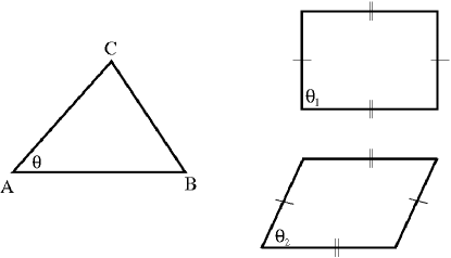
Figure 4: Rigidity of simplexes and their use in RC : (Left) A typical triangle $ABC$ in a 2-dimensional Delaunay lattice. One need only specify the lengths of its three edges, $\overline{AB}$, $\overline{AC}$ and $\overline{BC}$, to uniquely determine the geometry of the triangle (simplex). In particular, the area of the triangle $\triangle_{ABC}$ and its internal angles $\sin{\theta}=2\triangle_{ABC}/\overline{AB}\,\overline{AC}$ are explicit functions of the length of its three edges. In this sense the 2-simplex is rigid. (Right) Even though the four edges of the rectangle (upper right) are specified, its internal angle $\theta_{1}$ is not uniquely determined. The rectangle can be collapsed to a parallelogram (lower right) while preserving the lengths of each of its four edges. This non-simplicial block is not rigid and ${\theta}_{1}\neq{\theta_{2}}$.

In RC the curvature of a Delaunay lattice is concentrated at its co-dimension two elements. We will refer to these foci of curvature as hinges, $h$. The hinges in a 2-dimensional lattice are the vertices, in three dimensions the components of the Riemann curvature tensor are concentrated along the edges, and in the four dimensions of spacetime the triangles are the hinges. In the remainder of this section we examine the construction of the components of the Riemann curvature tensor on simplicial lattices first in 2-dimensions, then in 3-dimensions and finally in 4-dimensions. We demonstrate that the Voronoi areas dual to the hinges provide a natural measure for the curvature.

In 2-dimensions the building blocks are triangles. The spacetime geometry interior to each triangle is flat. Curvature, when present, is only concentrated at each vertex (co-dimension 2). The curvature represents a conic singularity. In other words, the net rotation of a vector when transported parallel to itself around a vertex hinge remains unchanged as one shrinks the closed loop. This constant rotation angle is referred to as the deficit angle ($\epsilon_{h}$).

Figure 5: Curvature is concentrated at the vertex hinges in two dimensions: (Left) The 2-dimensional triangular tessellation approximates triple torus. Here we examine the curvature concentrated at a particular vertex of this triple torus. (Right) When we magnify the vertex, we find it is the meeting place of six triangles, and that these six triangles form a convex hull. To flatten these six triangles onto a Euclidean plane the hull need to split along one of its edges. This angle of split, or deficit angle, captures the conic curvature. The deficit angle associated with a vertex is revealed as the sum of the internal angles’ difference from $2\pi$. The Voronoi area dual to the vertex (the shaded area) gives a natural closed loop for the definition of the Gaussian curvature.

$$\underbrace{\epsilon_{h}=2\pi-\sum_{i=1}^{6}\theta_{i}}_{\begin{array}[]{c}Deficit\,Angle\\ Angle\,Vector\,Rotates\end{array}}$$ (8)

Here $\theta_{i}$ is the internal angle of the $i^{\prime}th$ triangle at vertex hinge $h$ as illustrated in Fig. 5. In order to calculate the curvature, an appropriate closed loop surrounding our vertex hinge must be chosen for parallel transport. Since the hinge represents a conic singularity, the Gaussian curvature is independent of the area of the loop enclosing the vertex; however, the Voronoi area dual to the vertex hinge represents a natural choice for this area. In 2-dimensions, this area gives a natural closed loop that does not overlap any other closed loops on the tessellated geometry. Furthermore, it represents the set of points on the simplicial lattice close to this vertex than to any other vertex. In this sense it provides a democratic measure of the area assigned to each hinge. Using the deficit angle and the dual Voronoi area, the curvature (2) takes the usual form.

$$K_{h}=\frac{\epsilon_{h}}{A^{*}_{h}}$$ (9)

In 3-dimensions the building blocks are tetrahedra. The interior of each of these base building blocks is flat, and curvature is concentrated on the co-dimension 2 edges of the tessellationon the edges of the simplicial lattice. As one transports a vector around a loop surrounding the edge, the vector ordinarily comes back rotated by an angle $\epsilon_{h}$ which is still given by (8) and shown in Fig. 6. However, the $\theta_{i}$’s now represent the dihedral angles of the $i$’th tetrahedron formed between its two triangular faces that share the hinge. Dual to the edges are the 2-dimensional Voronoi areas, which will again play the role of loops for parallel transport as they still represent a proper tiling of the spacetime, as well as a natural weighting for each hinge. The curvature ${}^{(3)}K_{h}$ takes the same form as in 2-dimensions and is shown below.

$${}^{(3)}K_{h}=\frac{\epsilon_{h}}{A^{*}_{h}}$$ (10)

Figure 6: Hinges in 3-dimensions: In 3-dimensions, curvature is concentrated along edges. (Left) The deficit angle, the deficit from 2$\pi$ in the sum of dihedral angles on the hinge, determines the angle by which a vector carried around a loop surronding the hinge comes back rotated. (Right) The dual to the edge is a 2-dimensional face of the Voronoi diagram associated with the triangulation. This area serves as a natural loop for determination of the curvature associated with the hinge.

The story remains similar in 4-dimensions. The 4-simplex of Fig. 2 takes over the role of Delaunay cells. The interior of the 4-simplices are flat spacetime, and curvature is then concentrated on the triangular faces of the 4-simplices. Curvature is now measured by parallel transporting a vector around the triangular faces of the Delaunay lattice, which ordinarily will come back rotated by the deficit angle $\epsilon_{h}$. This deficit angle remains of the form of (8) where the $\theta_{i}$’s are now interpreted as the hyper-dihedral angles between tetrahedral faces of the $i$’th 4-simplex sharing the triangular hinge. Dual to the triangular hinges are still the 2-dimensional Voronoi faces, which again provide a natural closed loop for parallel transport. Taking the deficit angle and the Voronoi area dual to the hinge, the curvature ${}^{(4)}K_{h}$ maintains its general character from the 2- and 3-dimensional forms.

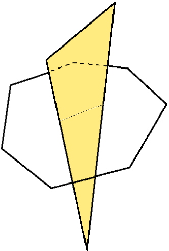
Figure 7: Hinges in 4-dimensions: In 4-dimensions, curvature is concentrated on co-dimension 2 triangular faces of the Delaunay lattice (shaded triangle). Dual to hinges are the 2-dimensional Voronoi faces (the heptagon in this example) which provide another natural area of closed parallel transport.

$${}^{(4)}K_{h}=\frac{\epsilon_{h}}{A^{*}_{h}}$$ (11)

Curvature in RC gives an example of the intertwined role that the Voronoi and Delaunay tessellations play in this discrete theory of spacetime. The Voronoi areas provide a natural loop for parallel transport while triangles of the Delaunay tessellation provide a framework for the definition of the angle rotated by a vector under parallel transport around the Voronoi area. We will see in the coming sections how the Voronoi and Delaunay lattices can be used to define curvature in a way that is compatible with observation and measurment.

4 A Fundamental Block Coupling the Voronoi and Delaunay Lattices Together

In the last section we emphasize that the curvature in a d-dimensional simplicial spacetime takes the form of a conic singularity at each point of the (d-2)-dimensional hinges (h). We noted that the deflection of a “d-axis gyroscope” when carried one complete circuit around a closed loop encircling a given hinge is indepedent of the area of the loop. We overcame this delimma in defining the curvature of the hinge by introducing the Voronoi area ($A_{h}^{*}$) dual to the hinge h as a natural and democratic measure for the distribution of this curvature. If there are $n$ d-dimensional simplexes sharing hinge h, then the Voronoi area ($A_{h}^{*}$) will be an $n$-gon (the heptagon in Fig. 7). Each corner of $h^{*}$ lies at the circumcenter of one of the d-simplexes in the Delaunay geometry which share h. We can connect the $n$ vertices of $h^{*}$ to the triangle to form a bi-pyramidal d-dimensional polytope. This forms a new fundamental lattice cell at each hinge h – a hybrid polytope built from elements from both the Voronoi ($h^{*}$) and Delaunay (h) hinges as shown in Fig. 8. This hybrid cell provides a proper tiling of the spacetime. Each hybrid cell having an $n$-gon $h^{*}$ can be deconstructed into $n$ d-simpexes, where each of these simplexes is formed by connecting an edge of $h^{*}$ with the (d-2) vertices of the co-dimension 2 simplicial hinge h. In this sense, they are rigid polytopes.

By construction, the Voronoi polygon $h^{*}$ is orthogonal to the hinge h. We use this orthogonality to show that the d-volume of these hybrid cells are simply proportional to the product of the d-area of the hinge ($A_{h}$) and the area ($A_{h}^{*}$) of its dual polygon $h^{*}$ M97 .

$$d^{(d)}V_{proper}=\frac{2}{d(d-1)}A_{h}A^{*}_{h}$$ (12)

This is a co-dimension 2 version of the usual formula for the area of a triangle as $\frac{1}{2}base\times altitude$. These dual hybrid Voronoi-Delaunay volume elements provide us with a natural decomposition for our Hilbert action as well as a natural structure to define the scalar curvature of any hinge, h.

Figure 8: The Hybrid Block: This definition of the hybrid block in RC forms a lattice of 4-dimensional blocks that incorporates many of the attractive features of the Delaunay and Voronoi lattices. These blocks naturally tile the spacetime and obtain rigidity from the underlying Delaunay lattice. Interpretations of these hybrid of blocks are ripe with analogs from solid state physics. The Delaunay lattice serves as a spacetime analog of the Bravais lattice so often found in the theory of solids. With this identification, the Voronoi cells might be considered analogs to the Brillouin zones for a non-periodic lattice. The hybrid block becomes a hybrid between a spacetime lattice and a fundamental lattice structure of momentum space. In anticipating future links with quantum theory, this leads us to consider this hybrid block as a precursor to a Wigner function on spacetime as it is precisely the Wigner function in standard quantum theory that attempts to link complementary variables into a qausi-probability function. In a similar manner, the hybrid block forms a unique lattice composed of complimentary lattices of spacetime.

The component of the Riemann curvature of this fundamental block is now naturally expressed in terms of its intrinsic geometry. It not only provides the orientation of the circumnavigated area ($A_{h}^{*}$), it also yields the curvature hinge and its orientation ($A_{h}$).

$$^{(d)}R_{h}=d(d-1)^{(d)}K_{h}=\frac{d(d-1)}{A^{*}_{h}}\epsilon_{h}$$ (13)

Four features of this representation of curvature at a hinge in Regge calculus are brought to the fore. First, the curvature is concentrated on the co-dimension 2 hinge, $h$. Second, the plane of rotation is perpendicular to the the hinge, $h$, which is a natural property inherited by the Voronoi-Delaunay duality. Third, and re-emphasizing this last point, the Voronoi polygon area $A^{*}_{h}$ is perpendicular to the hinge $h$, and provides a natural democratic weighting for the definition of the distribution of the conical singularity. Finally, and most importantly, locally the Regge spacetime is an Einstein space in that the Riemann tensor is proportional to the scalar curvature. This last property is again a direct consequence of the relationship of the dual lattices. The invariance in the orientation and magnitude of the rotation bi-vector with respect to the orientation of the dual area circumnavigated gives this remarkable property that the lattice spacetime in RC is locally an Einstein space E25 i.e.

$$R_{\mu\nu}=\frac{R}{d}\,g_{\mu\nu}.$$ (14)

This feature also gives the trace factor of $d(d-1)$ in front of the Gaussian curvature of (13).

Given this expression for the curvature at a hinge $h$ in a lattice spacetime, the derivation of the RC action is direct. Substituting the curvature expression (13) and the fundamental volume (12) into the Hilbert action (5).

$$\frac{1}{16\pi}\sum_{hinges,\ h}\left(\frac{d(d-1)}{A^{*}_{h}}\epsilon_{h}\right)\left(\frac{2}{d(d-1)}A_{h}A^{*}_{h}\right)$$ (15)

Canceling the obvious terms, we arrive at Tullio Regge’s expression for the Hilbert action for the lattice geometry. The Voronoi areas cancel leaving only the simplicial (Delaunay) objects behind.

$$I_{R}=\frac{1}{8\pi}\sum_{\begin{array}[]{c}triangle\\ hinges,\,h\end{array}}A_{h}\epsilon_{h}$$ (16)

While Voronoi lattice structure is absent from the Regge action, and absent from the vacuum spacetime Regge-Einstein equations, the Voronoi lattice is necessary for the curvature, the Einstein tensor, or the coupling of non-gravitational sources to RC.

The RC version of Einstein’s equations can now be obtained by variation of this action with respect to the proper lengths of the edges in the simplicial Delaunay spacetime lattice.

$$\delta(I_{R}) = \delta\left(\sum_{hinges,\,h}A_{h}\epsilon_{h}\right)$$ (17)

$$= \sum_{hinges,\,h}\delta(A_{h})\epsilon_{h}+\underbrace{\sum_{hinges,\,h}A_{h}\delta(\epsilon_{h})}_{zero}=0$$ (18)

In the continuum the Hilbert action is varied with respect to the metric components to yield the Einstein tensor (5, 6). However in RC we vary the Regge-Hilbert action (16) with respect to the edge lengths to obtain the corresponding RC equation (20). The variation of the triangle area ($A_{h}$) with respect to edge $L$ is expressed in terms of $L$ and the interior angle ($\theta_{h}$) of triangle $h$ opposite the edge $L$.

$$\delta(A_{h})=\frac{\partial A_{h}}{\partial L}\delta(L)=\frac{1}{2}L\cot(\theta_{h})$$ (19)

Regge showed in his original paper that the second term in (17) automatically vanishes R61 . This RC action principle yields one equation per edge ($L_{i}$) in the Delaunay simplicial lattice.

$$\underbrace{\sum_{\begin{array}[]{c}hinges,\ h\\ sharing\,edge\,L\end{array}}\frac{1}{2}L_{i}\cot(\theta_{h})\epsilon_{h}=0}_{\mbox{\small Regge equation associated with edge }L_{i}}$$ (20)

It is rather amazing to us that an identical equation can be obtained directly from the lattice by using the approach first introduced by E. Cartan (Fig. 9). Recall that the Einstein tensor has two components (1).

$$G=^{*}R^{*}=\underbrace{e_{\mu}}_{\begin{array}[]{c}Moment\\ of\\ Rotation\end{array}}G^{\mu}_{\nu}\underbrace{dx^{\nu}}_{3-volume}$$ (21)

In plain language, the second component of the Einstein tensor is identified with an oriented infinitesimal 3-volume. i.e. components of the 4-vector orthogonal to the 3-volume. The other component, Cartan showed, can be constructed using the rotation operator, as a sum of moments-of-rotation for each face of this 3-volume. This Cartan approach was applied to RC by one of us (M86 ) and demonstrates the need to incorporate the Voronoi 3-volumes dual to the Delaunay edges in order to define a precise expression for the Einstein tensor (Fig. 9). In RC the 3-volumes upon which we construct the Einstein tensor are naturally the Voronoi polyhedrons. Given an edge $L$ in the Delaunay lattice, one can identify its unique polyhedron of 3-volume $V^{*}_{L}$ in the circumcentric-dual Voronoi lattice. The RC version of the Einstein tensor associated to edge $L$ is identical to the equation we obtained from the action (20) divided by the corresponding Voronoi 3-volume.

$$G_{LL}\,V^{*}_{L}=\sum_{hinges,\,h}\underbrace{\frac{1}{2}L\cot(\theta_{h})}_{moment\,arm}\underbrace{\epsilon_{h}}_{rot^{\prime}n}$$ (22)

In addition, the introduction of the Voronoi lattice as demanded by the Cartan approach gives a simple geometric explanation of why there is only one Einstein tensor component per edge in the lattice geometry M86 . Again, the orthogonality of the Voronoi and Delaunay lattices demand this. The moment-of-rotation vector for each face of $V^{*}_{L}$ is oriented along edge $L$. Therefore the sum of the moment of rotation vectors is parallel to $L$, and the orientation of Voronoi 3-volume, by definition, is parallel to $L$. This is a direct consequence of the mutual orthogonality that exists between each element and its dual in the Voronoi-Delaunay lattices. We have, in RC, a purely geometric construction of the Einstein tensor associated with edge $L$ and it is diagonal along the edge. The RC equations requires elements from both the Delaunay and Voronoi lattices.

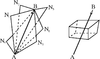
Figure 9: Cartain Approach to RC: The Voronoi polyhedral cells in the Voronoi lattice dual to the Delaunay lattice is a natural domain in RC for E. Cartan’s description of the Einstein tensor. In particular, in a vacuum spacetime, it yields the same Regge equation as is obtained from the variational principle. Left: A particular edge $L=AB$ in the simplicial Delaunay geometry ${\cal D}$ with its entourage of six triangles surrounding it. Some edges in ${\cal D}$ may have more or less triangles that it belongs to; however it must have at least four in which case the Voronoi polygon will be a tetrahedron. The orientation of $L$ is indicated by the arrow reaching from point A to point B. The orientation of $L$ ($A$ before $B$) induces an orientation on each of the six triangles ($A$ before $B$ before $N_{i}$). Right: This orientation also produces an orientation on the warped cube in the Voronoi lattice ${\cal V}$ dual to edge $L$ in ${\cal D}$. There is a 1-1 correspondence between any given square face on the cube and the corresponding triangle $A,B,N_{i}$. The perimeter of each square face of the warped cube in $V_{L}$ is to be thought of as the closed loop encircling the corresponding triangle hinge $ABN_{i}$. Since the Voronoi lattice ${\cal S}^{*}$ is the circumcentric dual of ${\cal S}$ then each vertex of the cube is located at the circumcenter of its corresponding simplex in ${\cal S}$.

The Einstein tensor is proportional to the stress-energy tensor. Therefore in RC the flow of stress-energy ($T_{LL}$) is directed along each edge. This we show elsewhere leads to a Kirchhoff-like conservation law at each vertex – the sum of the flow of energy-momentum into and out-of each vertex in the Delaunay lattice must be zero. The vanishing of this flow of energy-momentum is a consequence of a topological identity – the boundary-of-a-boundary is zero (W82 ).

In this section we demonstrate the indispensability of both the Voronoi and Delaunay structures in RC. The geometric laws of gravitation led us to couple these lattices and form a new, and perhaps, more fundamental tiling of the spacetime with hybrid polytopes. In the next sections to follow, we reinforce this unique marriage between the Voronoi and Delaunay lattices and provide the first geometric construction of the scalar curvature invariant at a vertex (event $v$ in spacetime) that we are aware of. In the next few sections we will use heavily the hybrid polytope and will introduce a reduced-version of this basic building block.

5 The Scalar Curvature Invariant in Regge Calculus

We have seen (5) that the Riemann scalar curvature invariant plays such a central role in Einstein’s geometric theory of gravitation. Its centrality in the theory cannot be over emphasized. The extremum of this quantity over a proper 4-volume of spacetime, yields a solution compatible with Einstein’s field equations. It is this scalar, so central to the Hilbert action, which yields the conservation of energy-momentum (contracted Bianchi identities) when variations are done with respect to the diffeomorphic degrees of freedom of the spacetime geometry. This scalar also augments the Ricci tensor in coupling the non-gravitational fields and matter to the curvature of spacetime. It not only appears in its 4-dimensional form in the integrand Hilbert action principle of GR, it makes its presence felt in 3-dimensions as an “effective potential energy” in the ADM action.

Given this curvature invariant’s pivotal role in the theory of GR, we believe it is important to understand how to locally construct this geometric object at a chosen event in an arbitrary curved spacetime. Given recent interest in discrete pre-geometric models of quantum gravity, it is ever so important to reconstruct the curvature scalar with respect to a finite number of observers and photonsL06 ; AJL06 . Even though we do have familiar discrete representations of each of the twenty components of the Riemann curvature tensor in terms of geodesic deviation or parallel transport around closed loopsS60 ; B66 ; CD86 , and apart from the sterile act of simply taking the trace of the Riemann tensor, we are not aware of such a chronometric construction of the scalar curvature.

We provide such a discrete geometric description of this scalar curvature invariant utilizing RC R61 ; MTW73 ; TW92 , and the convergence-in-mean of RC rigorously demonstrated by Cheeger, Müller and Schrader CMS84 . In the spirit of quantum mechanics and recent approaches to quantum gravity, our construction uses only clocks and photons local to an event on an observer’s world line. Furthermore, this construction is based on a finite number of observers (clocks) exchanging a finite amount of information via photon ranging and yields the scalar curvature naturally expressed in terms of Voronoi and Delaunay latticesbook . We pointed out in the first section of this paper that that these lattices naturally arise in RC CDM89 ; FL84 ; FFLR84 ; CFL82 ; CFL82b ; L83 ; HW86 ; HW86b ; M86 ; M97 .This constriction further emphasizes the fundamental role that Voronoi and Delaunay lattices have in the discrete representations of spacetime which is perhaps not so surprising given its preponderant role in self-evolving and interacting structures in naturebook . In this analysis we re-utilize the new hybrid (half Voronoi, half Delaunay) simplex (Fig. 8).

The key to our derivation of the Riemann-scalar curvature is the identification $I_{R}\equiv I_{V}$ of the usual hinge-based expression the RC version of the Hilbert action principle R61 ; M97 with its corresponding vertex-based expression. We begin with the Hilbert action in a $d$-dimensional continuum spacetime, which is expressible as an integral of the Riemann scalar curvature over the proper $d$-volume of the spacetime.

$$I=\frac{1}{16\pi}\int R\ dV_{proper}$$ (23)

On our lattice spacetime, and following the standard techniques of RC, we can approximate this action as a sum over the triangular hinges $h$.

$$I\approx I_{R}=\frac{1}{16\pi}\sum_{hinges,\ h}R_{h}\ \Delta V_{h}$$ (24)

Here, $R_{h}$ is the scalar curvature invariant associated to the hinge, and $\Delta V_{h}$ is the proper 4-volume in the lattice spacetime associated to the hinge $h$. Following earlier work by the authorsM97 , this curvature is defined explicitly. Though, non-standard in RC, we may also express the action in terms of a sum over the vertices of the simplicial $d$-dimensional Delaunay lattice spacetime.

$$I\approx I_{V}=\frac{1}{16\pi}\sum_{vertices,\ v}R_{v}\ \Delta V_{v}$$ (25)

It is the Riemann scalar curvature ($R_{v}$) at the vertex $v$ that appears in this expression that we seek in this manuscript, and it is the equivalence between (24) and (25) that will yield it. But first we must use the orthogonality inherent between the Voronoi and Delaunay lattices to determine the relevant 4-volumes ($\Delta V_{v}$ and $\Delta V_{h}$).

Consider a vertex $v$ in the Delaunay lattice, and consider a triangle hinge $h$ having vertex $v$ as one of its three corners. We define $A_{hv}$ to be the fraction of the area of hinge $h$ closest to vertex $v$ than to its other two vertices (Fig. 10). Dual to each triangle hinge, and in particular to triangle $h$, is a unique co-dimension 2 area, $A^{*}_{h}$, in the Voronoi lattice. This area necessarily lies in a $(d-2)$-dimensional hyperplane orthogonal to the 2-dimensional plane defined by the triangle $h$. The number of vertices of the dual $(d-2)$-polygon, $h^{*}$, is equal to the number of $d$-dimensional simplicies hinging on triangle $h$, and is always greater than or equal to three. If we join each of three vertices of hinge $h$, with the all of vertices of $h^{*}$ with new edges, then we naturally form a $d$-dimensional proper volume associated to with vertex $v$ and hinge $h$. This $d$-dimensional polytope is a hybridization of the Voronoi and Delaunay lattices, they completely tile the lattice spacetime without gaps or overlaps, and they inherent their rigidity from the underlying simplicial lattice.

$$\Delta V_{hv}\equiv\frac{2}{d(d-1)}\,A_{hv}A^{*}_{h}$$ (26)

The simplicity of this expression (the factorization of the simplicial spacetime and its dual) is a direct consequence of the inherent orthogonality between the Voronoi and Delaunay lattices, and its impact on this calculation, and in RC as a whole, cannot be overstated. These d-cells are the Regge-calculus hybrid versions of the reduced Brillouin cells commonly found in solid state physics, though they are hybrid because they are coupled to their dual structures in the underlying atomic lattice. We view these as the fundamental building blocks of lattice gravity and at the Planck scale perhaps the RC version of Leibniz’s Monads – Vinculum Substantiale. The scalar factor in this expression, which depends on the dimension of the lattice, was derived in the appendix of an earlier paper M97 . Furthermore we obtain the complete proper $d$-volume, $\Delta V_{v}$, by linearly summing (26) over each of the triangles $h$ in the Delaunay lattice sharing vertex $v$.

$$\Delta V_{v}=\sum_{h_{|v}}\Delta V_{hv}=\frac{2}{d(d-1)}\sum_{h_{|v}}A_{hv}A^{*}_{h}$$ (27)

We now can re-express the Regge-Hilbert action at a vertex in terms of these hybrid blocks.

$$I_{V}=\frac{1}{16\pi}\sum_{v}R_{v}\sum_{h_{|v}}\frac{2}{d(d-1)}A_{hv}A^{*}_{h}$$ (28)

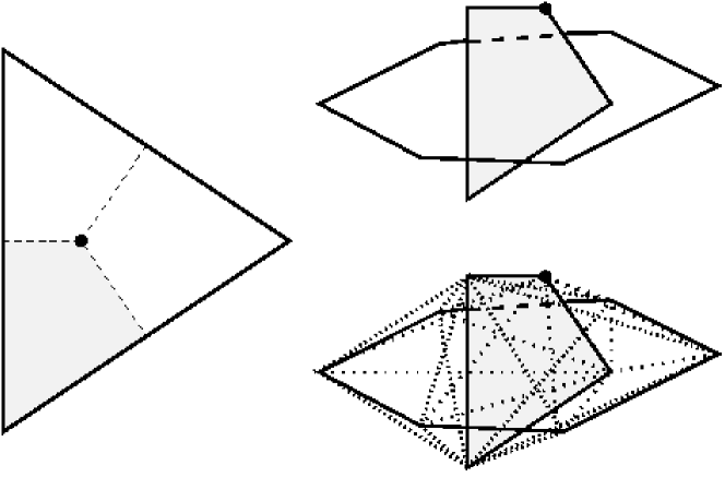
Figure 10: Reduced Hybrid d-cell: The triangle hinge $h$ to the left is partitioned into three areas. The shaded region ($A_{hv}$) represents the portion of the triangle that is closer to the lower vertex than its other two vertices. The darkened and pronounced vertex appearing in each of the three line drawings of this figure is the circumcenter of the hinge, $h$. Each hinge has its corresponding 2-dimensional dual Voronoi area ($A^{*}_{h}$) shown in the upper right part of the figure as a pentagonal shaped polygon, and illustrate this dual area as “encircling” the $d$-dimensional “kite” hinge. In bottom right portion of the figure, the “kite” hinge is connected to its dual Voronoi polygon by ($4\times 6=24$) new lattice edges – thus forming the reduced Voronoi-Delaunay hybrid d-cell which is fundamental to our derivation, the derivation of the Hilbert action in Regge calculus, and, we believe, fundamental to any discrete representation of gravitation. Each if these edges, as well as the edges of the Voronoi area are algebraic functions of the original Regge simplicial (Delaunay) lattice spacetime, and accordingly we have not added or subtracted any degrees of freedom. These new hybrid d-cells provide a new, and proper tiling of the lattice spacetime.

6 Obtaining the Scalar Curvature at a Vertex

We now return to the more familiar hinge-based Regge-Hilbert action ($I_{R}$) of (24). The proper 4-volume associated to hinge $h$ has been shown to be factorable in terms of the area of the triangle hinge and its corresponding dual Voronoi area M97 . Recall,

$$\Delta V_{h}=\frac{2}{d(d-1)}A_{h}A^{*}_{h}.$$ (29)

Following the procedure discussed above, we can express the area of $h$ as a sum of its circumcentrically-partitioned pieces (Figure 10).

$$A_{h}=\sum_{v_{|h}}A_{hv}$$ (30)

Therefore the action per hinge (24) can be expressed as the following double summation:

$$I_{R}=\frac{1}{16\pi}\sum_{h}\sum_{v_{|h}}R_{h}\left(\frac{2}{d(d-1)}A_{hv}A^{*}_{h}\right)$$ (31)

A key step in this derivation is the ability to switch the order of summation, and fortunately action is unchanged if we reverse this order.

$$I_{R}=\frac{1}{16\pi}\sum_{v}\sum_{h_{|v}}R_{h}\left(\frac{2}{d(d-1)}A_{hv}A^{*}_{h}\right)$$ (32)

The vertex-based action of (28) must be equal to this hinge-based action of (32). We immediately obtain the desired expression for the Riemann scalar curvature at a vertex.

$$R_{v}=\frac{\sum_{h_{|v}}R_{h}A^{*}_{h}A_{hv}}{\sum_{h_{|v}}A^{*}_{h}A_{hv}}=\frac{\sum_{h_{|v}}R_{h}A^{*}_{h}A_{hv}/\sum_{h_{|v}}A_{hv}}{\sum_{h_{|v}}A^{*}_{h}A_{hv}/\sum_{h_{|v}}A_{hv}}$$ (33)

Here we have divided the numerator and denominator by the same quantity leaving it unchanged. Both the numerator and denominator are in the form of a weighted average over the ”Brillion kites” ($A_{hv}$) at vertex $v$. We define, in a natural way, the “kite weighted average” at vertex $v$ of any hinge-based quantity $Q_{h}$ as follows:

$$\langle Q\rangle_{v}\equiv\frac{\sum_{h_{|v}}Q_{h}A_{hv}}{\sum_{h_{|v}}A_{hv}}.$$ (34)

Given this definition, the scalar curvature invariant at vertex $v$ can be expressed as a “kite-weighted average” of the integrated hinge-based scalar curvature of RC.

$$R_{v}=\frac{\langle R_{h}A^{*}_{h}\rangle_{v}}{\langle A^{*}_{h}\rangle_{v}},$$ (35)

where it was shown in M97 that the Riemann scalar curvature at the hinge $h$ is expressible as the hinge’s curvature deficit ($\epsilon_{h}$) per unit Voronoi area ($A^{*}_{h}$) dual to $h$.

$$R_{h}=\frac{1}{d(d-1)}\frac{\epsilon_{h}}{A^{*}_{h}}.$$ (36)

Therefore the expression for the vertex-based scalar curvature invariant derived here is strikingly similar to the usual Regge calculus expression for the hinge-based scalar curvature invariant (36). The only difference is that the numerator and denominator of (36) is replaced by their kite-weighted averages.

$$R_{v}=\frac{1}{d(d-1)}\frac{\langle\epsilon_{h}\rangle_{v}}{\langle A^{*}_{h}\rangle_{v}}$$ (37)

7 Convergence in Mean to the Continuum: An Example

The importance of the Voronoi and Delaunay dual tessellations in Regge calculus has been emphasized through their role in fundamental quantities such as the scalar curvature. Such vital quantities in the discrete theory should also lead to a continuum limit in some appropriate sense of convergence. It is not at all clear from a first look that this measure of the scalar curvature will indeed sufficiently approximate an appropriate smooth geometry. Fortunately, the result, proven earlier CMS84 , guaruntees this convergence. Consider a triangulation of a smooth geometry, say $S^{2}$, where the triangulation may be as fine or coarse as is desired. As shown in Sec. (2), the Gaussian curvature of the 2-sphere is given by $1/R^{2}$. Suppose, then, that instead of the smooth geometry of the 2-sphere, the geometry is given by a triangulated approximation to $S^{2}$. In what sense does a triangulated approximation converge to the smooth geometry?

As we alluded to, this question was investigated in full mathematical rigor in 1984 by Cheeger, Müller and Schrader CMS84 . In their analysis of RC’s convergence to the continuum, the piecewise flat approximation to a smooth geometry is refined into ever finer meshes via some subdivision algorithm. Although refinement of the triangulation becomes finer and the edge lengths tend towards zero, the curvature of the triangulation may not converge in a local sense, that is, at any given vertex on the triangulation, the curvature may vary, sometimes greatly, from the smooth geometry. Instead, a sense of convergence is obtained through considering extended regions of the triangulation. Convergence comes about in the sense of convergence in the mean, a common theme in many examples of discrete approximations to smooth functions. In the case of RC, the local curvature may fluctuate as one moves from one vertex to the other, yet given a extended region of the triangulation, a mean curvature does converge to the smooth geometry. A numerical calculation makes this idea of convergence of the discrete geometry to the smooth geometry abundantly clear.

Figure 11: The Geodetic Subdivision of an Icosahedron: From left to right are the n=0, n=1, and n=2 frequency geodetic subdivisions of the icosahedron, with their face subdivisions shown below the triangulated 2-sphere.

Suppose that as a first approximation to the sphere, an inscribed icosahedron is used as the triangulation, of course one could choose any other starting triangulation without any loss of generality. Then, using some subdivision algorithm, the initial triangulation is subdivided in progressively finer triangulations. Fig. 11 shows a geodetic subdivision of progressively finer triangulations of the $S^{2}$. This geodetic subdivision is accomplished through taking each face of the icosahedron and dividing that face into a grid, also shown in Fig. 11. Finer triangulations of $S^{2}$ are accomplished by taking finer meshes on the icosahedral faces. In order to keep the triangulations as approximations to the smooth geometry, the new vertices are then projected out to the surface of the sphere. The lengths assigned to the triangulation are the geodesic lengths of their projections on surface. In this way, a finer, and still uniform, triangulation of the smooth spherical geometry is obtained. In two dimensions, the curvature is concentrated on the vertices of the triangulation, and the Voronoi polygon associated with that vertex provides a natural loop for parallel transport. When the curvature is calculated for the vertices of the triangulation of a finely triangulated geodesic dome, one gets as expected the 1/$R^{2}$ curvature; however, local fluctuations are present (Fig. 12). This calculation concretely shows that the curvuture associated with the vertices of the triangulation does not locally converge to the curvature of the smooth geometry; however, the curvature of the triangulation does fluctuate around the smooth geometry’s curvature. It is in this sense that the curvature of the triangulation converges in the mean.

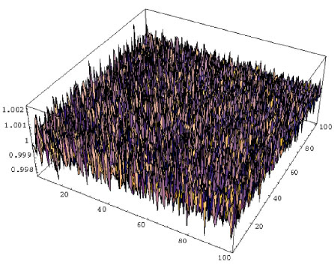
Figure 12: Convergence in Mean: For a sufficiently fine triangulation of the 2-sphere, the curvature at a vertex-hinge of the lattice may not converge to the curvature of the sphere locally. This plot of the vertex curvature times the square of the radius of the sphere should return the continuum value of unity. However, across a region of an n=6 tessellated sphere, deviations from smooth curvature are clearly present ($K_{v}R^{2}=1\pm 0.002$). Convergence to the smooth curvature is seen to be obtained in mean through considering the average curvature over extended regions on the surface.

8 The Fundamental Role of Voronoi and Delaunay Lattices in Discrete Gravity and Future Directions

One can’t help but notice how widespread and natural the Voronoi and Delaunay structures are in nature. The vast number of applications described in these proceedings substantiate this as well as their potential universality. We further reinforce this property by demonstrating that they appear to be indispensable in providing a discrete representation of gravity, which many would consider the most fundamental interaction in nature. MW57 What we glean from nature should, in the end, boils down to bit-by-bit quantum measurements. As Wheeler would re-emphasize over and over to us; “No elementary quantum phenomenon is a phenomenon, unless it is brought to close by an irreversible act of amplification.” It-from-Bit These principles stand as our guide here in studying discrete models of the fundamental forces in nature.

We analyzed here, in great depth, the inner workings of RC and its natural expression in terms of a hybridization of the Voronoi and Delaunay lattices. In RC the principles of GR are applied directly to the lattice spacetime geometry. We analyzed the structure of curvature on a simplicial lattice, the RC form of the Hilbert action of GR and studied the structure of the Einstein tensor. Each of these central facets of GR require the Voronoi and Delaunay lattices for their definition. However, what is even more surprising to us is that the theory naturally yields a representation of spacetime by lattice cells which inherit properties from both the Voronoi and Delaunay lattices.

Two aspects raised here may provide us with a clue as to how nature works at the quantum level. First, the dual hybrid lattice provides a natural and fundamental hybrid building block describing the dynamics of the gravitational field. Second, the underlying discrete theory of gravity appears more austere via the underlying factorization of the hybrid volume elements; however, the full theory is recovered by convergence in mean. It is these clues that we sought in this paper. Will a unified theory of nature need to have these properties?

The hybrid block captures curvature. It promotes the Voronoi area to “center stage” as a natural dynamical variable in GR. this is hardly a new concept BRW99 ; M94 ; R93 ; R98 ; A86 , but it does provide a new perspective to a field that has been struggling with making a natural area-formulation of gravitation work. Anlong this line, we ask; “Can the Voronoi-Delaunay structure provide a foundation to incorporate the quantum principle of complementarity in quantum gravity”? Perhaps the duality between the Voronoi elements and the Delaunay elements provides a natural setting for the quantum principle of complementarity, and perhaps the democratic partitioning of volume supplies one with a natural topological structure, and that dual areas are natural placeholders for the quantum Aharovov-Bohm phases in GR , which yield the graviton fields.

References

- (1) T Regge: Nuovo Cimento 19, 558 (1961)
- (2) P.A. Tuckey, R.M. Williams: Class. Quantum Grav. 9, 1409-1422 (1992)
- (3) A. Okabe, B. Boots, K. Suqihara, S. N. Chiu: Spatial Tessellations: Concepts and Applications of Voronoi Diagrams 2nd ed. (John Wiley & Sons Ltd., West Sussex 2000)
- (4) J. Cheeger, W. Müller, R. Schrader: Lecture Notes in Phys. 160, 176-188 (1982)
- (5) J. Cheeger, W. Müller, R. Schrader: Commun. Math. Phys. 92, 405 (1984)
- (6) H. Hamber: Simplicial Quantum Gravity. In: Gauge Theories, Critical Phenomena and Random Systems: Proceedings of the 1984 Les Houches Summer School, Session XLIII, ed by K. Osterwalder, R. Stora (North Holland, Amsterdam 1986)
- (7) W.A. Miller: Found. Phys. 16, 143-169 (1986)
- (8) P.A. Morse: Class. Quantum Grav. 9, 2489-2504 (1992)
- (9) T.D. Lee: Phys. Lett. B122, 217-220 (1982)
- (10) C.W. Misner, K.S. Thorne, J.A. Wheeler: Gravitation (W. H. Freeman and Company, New York 1973) ch 42
- (11) L.P. Eisenhart Riemannian Geometry (Princeton Univ. Press, Princeton 1925) Ch. 2
- (12) J.A. Wheeler: Particles and geometry. In Unified Theories of Elementary Particles, (Springer-Verlag, San Francisco 1982) ed by Breithenlohner, H. Durr pp. 189-217
- (13) S. Lloyd: “A theory of quantum gravity based on quantum computation” arXiv:quant-ph/0501135 (2006)
- (14) J. Ambjorn, J. Jurkiewicz, R. Loll: “Quantum gravity: the art of building spacetime” arXiv:hep-th/0604212v1 (2006)
- (15) L. Synge: Relativity, The General Theory (North Holland, Amsterdam 1960) p 408
- (16) B. Bertotti: J. Math. Phys. 7, 1349 (1966)
- (17) I. Ciufolini, M. Demianski: Phys. Rev. D34, 1018-1020 (1986)
- (18) M. Castelle, A. D’Adda, L. Magnea Phys. Lett B232, 457 (1989)
- (19) R. Friedberg, T.D. Lee: Nucl. Phys. B242 p 145 (1984)
- (20) G. Feinberg, R. Friedberg, T.D. Lee, H. C. Ren: Nucl. Phys. B245, 343 (1984)
- (21) N.H. Christ, R. Friedberg, T.D. Lee: Nucl. Phys. B202, 89 (1982)
- (22) N.H. Christ, R. Friedberg, T.D. Lee: Nucl. Phys. B210, 337 (1982)
- (23) T.D. Lee, Phys. Lett. B122, 217 (1983)
- (24) H. Hamber, R.M. Williams: Nucl. Phys. B267, 482 (1986)
- (25) H Hamber, R. M. Williams: Nucl. Phys. B248, 392 (1986)
- (26) W.A. Miller: Class. Quantum Grav. 14, L199-L204 (1997)
- (27) C. W. Misner, J. A. Wheeler, Ann. Phys. 2, 525-603 (1957)
- (28) J. A. Wheeler, Information, Physics, Quantum: The Search for Links. in: Complexity, Entropy, and the Physics of Information, ed. by W. H. Zurek (Addison-Wesley, Redwood City, CA 1990) pp. 3-28. (1990).
- (29) J. W. Barrett, M. Rocek, R. M. Williams, Class. Quantum Grav. 16, 1373-1376 (1999)
- (30) J. Mäkelä, Phys. Rev. D49, 2882 (1994)
- (31) C. Rovelli, Phys. Rev. D48, 2702 (1993)
- (32) C. Rovelli, Living Rev. Rel. 1, 1 (1998)
- (33) A. Ashtekar, Phys. Rev. D 36, 1587-1602 (1986)