Next to Leading Order Spin(1)Spin(1) Effects in the Motion of Inspiralling Compact Binaries

Abstract

Using effective field theory techniques we compute the next to leading order Spin(1)Spin(1) terms in the potential of spinning compact objects at third Post-Newtonian (PN) order, including subleading self-induced finite size effects. This result represents the last ingredient to complete the relevant spin potentials to 3PN order from which the equations of motion follow via a canonical formalism. As an example we include the precession equation.

I Introduction

There has been significant progress in calculating higher order corrections to the potentials for spinning compact binaries. The spin potentials to 3PN order, from which the ${\cal O}({\bf S}_{1}{\bf S}_{2})$ contribution to the equations of motion (EOM) follow via a canonical procedure, were reported in eih for direct spin–spin interactions, and in comment from indirect spin–orbit effects. These results were presented using the Newton-Wigner (NW) spin supplementarity condition (SSC) at the level of the action. The latter procedure was shown to be accurate up to 4PN order in nrgr5 using standard power counting techniques. These results were derived using the NRGR formalism, which appears to provide simple tools to compute in the PN expansion nrgr ; nrgr1 ; nrgr2 ; nrgr3 ; nrgr4 ; nrgr5 ; nrgr6 , as well as the extremal limit workadam ; chad . More recently we computed the spin potentials to 3PN order in the covariant SSC ss , and explicitly showed the equivalence with our previous results in eih ; comment . The computations using the NW SSC at the level of the action were also re-derived within the NRGR approach in levi , albeit using a different choice of metric parameterizations introduced in kol2 . A recent calculation of the ${\bf S}_{1}{\bf S}_{2}$ Hamiltonian to 3PN appeared in Schafer3pn . The results in Schafer3pn helped to clarify the necessity of taking into account spin–orbit effects to compute the ${\cal O}({\bf S}_{1}{\bf S}_{2})$ contributions in the EOM to 3PN when one is working with the SSC at the level of the action. The equivalence between ours, and the more traditional approach of Schafer3pn , was shown in comment ; ss .

In ss we worked within a Routhian formalism originally introduced in yee , and developed in nrgr5 ; ss within NRGR, which incorporates the (covariant) SSC and its conservation upon evolution in a canonical framework to all orders. Within the formalism of nrgr5 ; ss the subleading spin–orbit effect in the EOM is proportional to $S^{j0}$, the spin tensor in the local frame, and contribute at ${\cal O}({\bf S}_{1}{\bf S}_{2})$ after one reduces spin to a three vector using the SSC and takes into account the transformation between the local and global PN frames. Ultimately, the equivalence between the independent results computed in eih ; comment and ss , with those in Schafer3pn using ADM techniques adm , confirms the validity of the new results at 3PN.

In ss we sketched the necessary steps towards computing the next to leading order (NLO) ${\cal O}({\bf S}_{i}^{2})$ contributions to the potential, which is the subject of this paper. We first review the Routhian approach, emphasizing the inclusion of higher dimensional operators and the preservation of the SSC under time evolution. We break up the calculation into three distinct types of contributions: The non–linear interactions, the finite size effects, and the contribution from the extra piece of the Routhian of ss , which must be included to insure that the SSC is preserved upon evolution. As an example we include the precession equation to 3PN. In appendix B we show how our result reduces to the geodesic motion around a Kerr background in the extreme mass ratio limit.

II NRGR and spin effects in the Routhian approach

One can introduce a Routhian to describe spin dynamics in a gravitational field as follows nrgr5 ; ss

$${\cal R}=-\sum_{q}\left(m_{q}\sqrt{u^{2}_{q}}+\frac{1}{2}S_{q}^{ab}\omega_{ab\mu}u^{\mu}_{q}+\frac{1}{2m_{q}}R_{deab}(x_{q})S^{cd}_{q}S^{ab}_{q}\frac{u^{e}_{q}u_{qc}}{\sqrt{u^{2}}}+\ldots\right),$$ (1)

where the ellipses represent non–linear terms in the curvature necessary to account for the mismatch between $p$ and $u$ once the SSC is enforced. Since at 3PN order we can consider the covariant SSC to be $S^{ab}u_{b}=0$, the higher order terms are irrelevant for our purposes. There is of course no obstruction to include higher order effects. The overall minus sign is chosen to ensure the spinless Feynman rules are not modified and the equations of motion (EOM) follow from

$$\frac{\delta}{\delta x^{\mu}}\int{\cal R}d\lambda=0,\;\;\;\frac{dS^{ab}}{d\lambda}=\{S^{ab},{\cal R}\},\;\;\;\frac{dS^{ab}}{d\lambda}=\{V,S^{ab}\},$$ (2)

where the potential is given by $V=-{\cal R}$, and

$$\{x^{\mu},{\cal P}_{\alpha}\} = \delta^{\mu}_{\alpha},\;\;\;\{x^{\mu},p_{\alpha}\}=\delta^{\mu}_{\alpha},\;\;\;\{{\cal P}^{\alpha},{\cal P}^{\beta}\}=0,$$ (3)

$$\{x^{\mu},x^{\nu}\} = 0,\;\;\;\{p^{\alpha},p^{\beta}\}=\frac{1}{2}{R^{\alpha\beta}}_{ab}S^{ab},$$ (4)

$$\{x^{\mu},S^{ab}\} = 0,\;\;\;\{p_{\alpha},S^{ab}\}=\omega^{c[a}_{\alpha}S^{b]c},\;\;\;\{{\cal P}^{\alpha},S^{ab}\}=0$$ (5)

$$\{S^{ab},S^{cd}\} = \eta^{ac}S^{bd}+\eta^{bd}S^{ac}-\eta^{ad}S^{bc}-\eta^{bc}S^{ad}$$ (6)

with $p^{\mu}$ given by ${\cal P}^{\mu}=p^{\mu}+\frac{1}{2}\omega^{\mu}_{ab}S^{ab}$, and ${\cal P}^{\mu}$ the canonical momentum. It is easy to show the Mathisson-Papapetrou equations papa follow from (2), and the Riemann dependent term in the Routhian guarantees the SSC is preserved upon evolution ss .

Notice that our Routhian is similar to the one introduced in yee , after the replacement

$$\frac{1}{2m_{q}}R_{deab}S^{cd}S^{ab}\frac{u^{e}u_{c}}{\sqrt{u^{2}}}\to\frac{1}{m_{q}}\frac{Dp^{d}}{d\lambda}\frac{S^{dc}u_{c}}{\sqrt{u^{2}}}.$$ (7)

The replacement in (7) follow from a change of variables. Furthermore, one can show that the net effect of this change yee modifies the spin-gravity coupling as follows

$$-\frac{1}{2}\omega_{\mu}^{ab}{S}_{ab}u^{\mu}\rightarrow-\frac{1}{2}\omega_{\mu}^{ab}{\cal S}_{ab}u^{\mu},$$ (8)

where

$${\cal S}^{ab}=S^{ab}+\frac{u_{c}}{u^{2}}S^{c[a}u^{b]},$$ (9)

or equivalently ($q=1,2$)

$${\cal S}_{q}^{i0}=S_{q}^{ij}v_{q}^{j}+\ldots$$ (10)

and

$${\cal S}^{ij}_{q}=S^{ij}_{q}+(S^{0i}_{q}-v_{q}^{k}S_{q}^{ki})v_{q}^{j}-(S_{q}^{0j}-v_{q}^{k}S_{q}^{kj})v_{q}^{i}+\ldots.$$ (11)

From here it easy to show that, when the Routhian is equivalently written in terms of $\cal S$ using (7), the covariant SSC is conserved, since

$$\frac{d}{dt}(S^{ab}u_{b})=u_{b}\{S^{ab},{\cal R}_{0}({\cal S}^{ab})\}+{\dot{u}}_{d}\frac{u_{c}}{u^{2}}\{S^{ab},S^{cd}\}u_{b}+S^{ab}{\dot{u}}_{b}=0,$$ (12)

where

$${\cal R}_{0}=-\sum_{q}\left(m_{q}\sqrt{u^{2}_{q}}+\frac{1}{2}{\cal S}_{q}^{ab}\omega_{ab\mu}u^{\mu}_{q}\right).$$ (13)

The expression in (12) follows from the identity

$$u_{b}\{S^{ab},{\cal R}_{0}({\cal S}^{ab})\}=0,$$ (14)

due to the fact that the spin algebra in terms of ${\cal S}^{ab}$ modifies the expression in (6) by shifting $\eta^{ab}\to\eta^{ab}-\frac{u^{a}u^{b}}{u^{2}}$. The inclusion of finite size effects obviously modify the EOM and the constancy of the SSC upon evolution is not guaranteed. However, from (12) and (14) it is clear that higher dimensional operators describing the internal structure of the bodies that are written in terms of ${\cal S}^{ab}$ will preserve the consistency of the covariant SSC as shown in yee .

In the NRGR formalism, physically relevant higher dimensional operators are those which are written in terms of the electric, $E_{ab}$, and magnetic, $B_{ab}$, components of the Weyl tensor nrgr ; nrgr2 ; nrgr3 ; nrgr6 . Terms which are proportional to the Ricci tensor, or scalar, can be removed by a field redefinition since they vanish on–shell nrgr . As we mentioned earlier, in order to preserve the SSC constraint upon evolution one needs to use ${\cal S}^{ab}$ for the higher dimensional terms in the wordline action. However, once these terms are written as a functions of the electric and magnetic part of the Weyl tensor, it is easy to show that using $S^{ab}$ still preserves the SSC, as a consequence of the SSC itself and the orthogonality relation, $E_{ab}u^{b}=B_{ab}u^{b}=0$. For example, the first higher dimensional operator we encounter is the self–induced quadrupole–like term, which written in terms of ${\cal S}^{ab}$ takes the form eih ; nrgr3 ; ss ($q=1,2$)

$$L_{E{\cal S}^{2}}=\frac{C^{(q)}_{ES^{2}}}{2mm_{p}}\frac{E_{ab}}{\sqrt{u^{2}}}{{{\cal S}}^{a}}_{c}{\cal S}^{cb}.$$ (15)

If we now take $L_{E{\cal S}^{2}}$ and expand ${\cal S}^{ab}$ in terms of $S^{ab}$ using (9) it is easy to show that the difference between (15) and

$$L_{ES^{2}}=\frac{C_{ES^{2}}}{2mm_{p}}\frac{E_{ab}}{\sqrt{u^{2}}}{{S}^{a}}_{c}S^{cb},$$ (16)

is proportional to $(S^{ab}u_{b})^{2}$ and therefore can be set to zero, given that it does not affect the EOM since it produces a correction which is proportional to the SSC itself. Therefore, we have a choice: we can use either (15) or (16), as they lead to the same result. In what follows we will use (16), although we will also provide the equivalent result using (15) in appendix A.

The operator in (16) reproduces the well known LO spin quadrupole contribution to the potential

$$V_{2PN}^{s^{2}}=-C^{(1)}_{ES^{2}}\frac{m_{2}}{2m_{1}r^{3}}\left({\bf S}_{1}\cdot{\bf S}_{1}-3{\bf S}_{1}\cdot{\bf n}{\bf S}_{1}\cdot{\bf n}\right)+1\to 2.$$ (17)

In the case of a rotating black hole $C_{ES^{2}}=1$, and this term represents the non–vanishing quadrupole moment of the Kerr solution. The coefficient for other compact objects can be calculated via a matching procedure. In this paper we will compute the corrections from (16) to the gravitational potential at 3PN. As we will show below there are no other contributions at 3PN from other higher dimensional operators.

By using the EFT power counting rules it is easy to organize the perturbative expansion in a systematic way. To obtain Post-Newtonian corrections one calculates ${\cal R}$, or the effective potential, perturbatively, without imposing the SSC (see ss for details). The advantage of this approach is that one does not have to worry about complicated algebraic structures. The price to pay is the need of a spin tensor rather than a three vector, though once we find the EOM via (2) we may write our results in terms of three vector and the coordinate velocity. For the former a precession equation can be obtained.

III Next to Leading Order $S^{2}$ potentials

The algorithm to calculate potentials in the EFT approach is quite simple. First of all we take all of the terms in the Routhian and collects them according to their order in the power counting (see nrgr ; nrgr3 for details of the power counting). Then we draw all possible Feynman diagrams at the order of interest. Each diagram is written in terms of a set of scalar integrals, and the diagram adds a term to the effective action given by $-i\int dtV$, where $V$ is the contribution of that diagram to the effective potential (see ss ). Throughout this section we will suppress the factors of “$\int dt$” in the diagrams. See TASI for details on EFTs.

III.1 Feynman rules: spin–graviton vertex

In the weak gravity limit the relevant spin couplings are nrgr3 ; eih ; ss

$$L^{NRGR}_{1PN} = \frac{1}{2m_{p}}H_{i0,k}S^{ik},$$ (18)

$$L^{NRGR}_{1.5PN} = \frac{1}{2m_{p}}\left(H_{ij,k}S^{ik}u^{j}+H_{00,k}S^{0k}\right),$$ (19)

$$L^{NRGR}_{2PN} = \frac{1}{2m_{p}}\left(H_{0j,k}S^{0k}u^{j}+H_{i0,0}S^{i0}\right)+\frac{1}{4m^{2}_{p}}S^{ij}\left(H^{\lambda}_{j}H_{0\lambda,i}-H^{k}_{j}H_{0i,k}\right).$$ (20)

We refer the reader to nrgr1 for all the other Feynman rules not involving spin.

III.2 $S^{2}$ terms from non–linear gravitational effects

The Feynman rules in (18,19,20) will contribute to the potentials terms which do not arise from either finite size effects or the Routhian term of the form $RSS$. These non-linear gravitational terms contribute from the diagrams shown in (1).

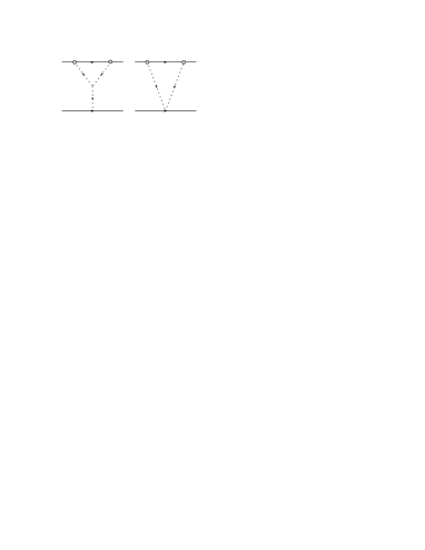
Figure 1: Non–linear $S^{2}$ terms. The blob represents a spin insertion.

It is easy to show that the “seagull” diagram (the one not containing the three graviton interaction) contributes at 4PN, since $\langle H_{00}H_{0i}\rangle=0$. (Where bracketed polynomials correspond to time ordered products and reduce down to retarded Greens function for quadratics.) Therefore, for the subleading non–linear $S^{2}$ effects the only non-vanishing contribution comes from the three graviton vertex which resides in the three point function, $\langle H_{00}H_{0i}H_{0j}\rangle$. This contraction can be easily handled by a short Mathematica routine which can be found at workshop . The result from the non–linear effects at 3PN is

$$\mbox{Fig.~{}\ref{nonl}}=i\frac{m_{2}G_{N}^{2}}{2r^{4}}S^{ik}_{1}S^{jk}_{1}(\delta^{ij}-2n^{i}n^{j})=i\frac{m_{2}G_{N}^{2}}{r^{4}}({\bf S}_{1}\cdot{\bf n})^{2},$$ (21)

from which we obtain the potential

$$V^{s^{2}}_{nl}=-\frac{m_{2}G_{N}^{2}}{r^{4}}({\bf S}_{1}\cdot{\bf n})^{2}.$$ (22)

III.3 $S^{2}$ terms from the Routhian

Recall that the Routhain includes a terms quadratic in the spin given by

$$L_{RS^{2}}=-\frac{1}{2m_{q}}R_{deab}(x_{q})S^{cd}_{q}S^{ab}_{q}\frac{u^{e}_{q}u_{qc}}{\sqrt{u^{2}}},$$ (23)

whose LO contribution shows up at 2.5PN,

$$L^{2.5PN}_{RS^{2}}=-\frac{1}{2m}R_{i0jk}S^{jk}S^{ci}v_{c}\sim\frac{1}{2m}H_{0k,ij}S^{jk}S^{ci}v_{c}.$$ (24)

To get a 3PN net effect we need to calculate a diagram similar to Fig. 3b, with the box representing now an insertion of $L_{RS^{2}}$, to produce a contribution

$$\langle L^{2.5PN}_{RS^{2}}(m_{2}H_{0i}v_{2}^{i})\rangle=i\frac{2m_{2}G_{N}}{m_{1}r^{3}}\left[3{\bf n}\cdot({\bf v}_{2}\times{\bf S}_{1})n^{l}-({\bf v}_{2}\times{\bf S}_{1})^{l}\right]S_{1}^{cl}v_{c}.$$ (25)

Also at 3PN we have a contribution from (23),

$$L^{3PN}_{RS^{2}}=\frac{1}{4m}\left(2H_{li,0j}S^{ij}+2H_{00,lj}S^{j0}-S^{ij}v^{k}(H_{lj,ki}+H_{ki,lj}-H_{li,kj}-H_{kj,li})\right)S^{cl}v_{c},$$ (26)

which contracts with a LO mass insertion to account for a 3PN contribution given by,

$$\langle L^{3PN}_{RS^{2}}(\frac{m_{2}}{2}H_{00})\rangle = -i\frac{m_{2}G_{N}}{m_{1}r^{3}}\left[\left({\bf v}_{2}-3{\bf v}_{1})\times{\bf S}_{1}\right)^{l}+6n^{l}({\bf v}_{1}\times{\bf S}_{1})\cdot{\bf n}+3({\bf n}\times{\bf S}_{1})^{l}({\bf n}\cdot{\bf v})\right]S_{1}^{cl}v_{c}.$$

Adding both pieces together we end up with the contibution to the potential,

$$V^{RS^{2}}_{3PN}=\left({\bf\tilde{a}}^{so}_{1(1)}\right)^{l}S_{1}^{cl}v_{1c}+1\to 2,$$ (28)

with ${\bf\tilde{a}}^{so}_{1(1)}$ the ${\bf S}_{1}$ piece of the acceleration in the local frame,

$${\bf\tilde{a}}^{so}_{1(1)}=\frac{m_{2}G_{N}}{m_{1}r^{3}}\left[-3{\bf v}\times{\bf S}_{1}+6{\bf n}({\bf v}\times{\bf S}_{1})\cdot{\bf n}+3{\bf n}\cdot{\bf v}({\bf n}\times{\bf S}_{1})\right].$$ (29)

Notice that we substituted the SSC for the $S_{1}^{j0}$ term inside the bracket in (26) since it multiplies the SSC itself. From here we can use (2) to obtain the EOM from which we get

$$\frac{d{\bf S}_{1}}{dt}=\ldots+({\bf\tilde{a}}^{so}_{1(1)}\times{\bf S}_{1})\times{\bf v}_{1}+\ldots$$ (30)

A similar expression straightforwardly follows by using the acceleration dependent form of the extra piece in the Routhian after the redefinition in (7).

III.4 Subleading $S^{2}$ terms from finite size effects

Let us now consider the finite size corrections. Using the power counting nrgr1 it is straightforward to show that the LO contribution from (16) scales $L_{ES^{2}}\sim\sqrt{L}v^{4}$, for maximally rotating compact objects, with $C_{ES^{2}}\sim 1$. As we mentioned before, this term generates a gravitational potential of the form of (17) at 2PN. As it is well known, rotating BHs or NSs have a quadrupole moments given by $Q_{bh}=-aS^{2}/m$ ($G=c=1$), with $m,S$, the mass and spin respectively mtw . For a BH we have $a=1$, and for NS $a$ ranges between $4$ and $8$ depending on the equation of state of the neutron star matter poisson2 . Matching this result with the effective theory we find $C_{ES^{2}}\equiv a$, which is consistent with what we expect from naturalness arguments. It also tells us that this contribution is enhanced for NSs with respect to BHs, since the latter seems to provide a lower bound for $C_{ES^{2}}$ in (16) .

In order to calculate the 3PN NLO correction due to the finite size of the objects we need to take care of two things: first we need to expand (16) in powers of the relative velocity $v$, and compute all possible $S^{2}$–orbit diagrams such that the net scaling goes like $v^{6}$; and second we have to make sure we are not missing any other higher dimensional operator which could contribute at 3PN order.

III.4.1 All Possible Higher dimensional operators

Let us start with the higher dimensional operators. At NLO we have a few operators that could contribute. Let us start using ${\cal S}^{ab}$ to begin with since its use guarantees the preservation of the SSC upon evolution. Furthermore, let us put aside reparameterization invariance (RPI) for the time being . If we define ${\cal S}^{a}=\epsilon^{abcd}{\cal S}_{bc}u_{d}$ we can write down the following new terms in the action

$$D_{a}B_{cd}{\cal S}^{ac}{\cal S}^{d},$$ (31)

$$D_{a}E_{cd}{\cal S}^{ac}{\cal S}^{d}.$$ (32)

where $B_{ab}$ represents the magnetic part of the Weyl tensor.

These terms are self–induced effects which can be generated by diagrams in the one–point function with two spin insertions. These operators scale as $\sqrt{L}v^{6}$ and $\sqrt{L}v^{7}$ respectively. Both will contribute beyond 3PN since the magnetic component of the Weyl tensor does not couple to a LO mass insertion, e.g. $\langle B_{ab}H_{00}\rangle=0$. We may wonder about operators with only two derivatives since we could also have

$$E_{bc}{\cal S}^{ab}u_{a}{\cal S}^{cd}u_{d}$$ (33)

$$B_{cb}{\cal S}^{ac}{\cal S}^{b}u_{a}.$$ (34)

Notice however that these operator cannot contribute since ${\cal S}^{ab}u_{b}\equiv 0$, identically. We could, however, have chosen to write these operators in terms of $S^{ab}$, in which case the first one does not contribute, since it is proportional to $(S^{ab}u_{b})^{2}$ and thus always has a vanishing contribution to the EOM. On the other hand, the second term in (34) would be equivalent to

$$R_{abcd}S^{bc}S^{de}u^{a}u_{e},$$ (35)

and we immediately recognize this is our extra term in the Routhian of (1). Notice that, once the SSC is enforced, this term does not contribute to the $n$–point function. This makes fixing its coefficient, by matching to the full theory, ambiguos. Which is to say that the coefficient is independent of the underlying theory and must be fixed algebraically. This is consistent with the fact that Wilson coefficient is fixed by the consistency of the SSC, in this case the covariant choice, as discussed in the previous section.

Finally we should consider the term

$$L_{BS^{2}}=C_{BS^{2}}B_{cd}S^{cb}S_{b}^{d},$$ (36)

similar to the electric quadrupole. The contribution of this operator to the potential stems from the coupling to an ${\cal O}(v)$ mass insertion of the form $H_{0i}v^{i}$. The LO potential at 2.5PN reads

$$V^{s^{2}}_{BS^{2}}=C_{BS^{2}}\frac{6G_{N}}{r^{3}}({\bf n}\times{\bf v}_{2})\cdot{\bf S}_{1}({\bf n}\cdot{\bf S}_{1})+1\to 2.$$ (37)

It turns out however that this term has a vanishing Wilson coefficient, e.g. $C_{BS^{2}}=0$, due to parity conservation. For instance we can easily show that it vanishes for the case of a Kerr BH by comparison with the multipole expansion of the Kerr metric in harmonic coordinates.

III.4.2 NLO corrections to the (spin²)quadrupole–monopole interaction induced by $L_{ES^{2}}$.

We are then left to compute the subleading corrections due to (16). Using the power counting rules of NRGR for spinning bodies nrgr3 we obtain the following new vertices

$$L_{ES^{2}}^{2PN} = -\frac{C_{ES^{2}}}{4mm_{p}}H_{00,ij}S^{ik}S^{jk},$$ (38)

$$L_{ES^{2}}^{2.5PN} = -\frac{C_{ES^{2}}}{2mm_{p}}H_{0l,ij}v^{l}S^{ik}S^{jk},$$ (39)

$$L_{ES^{2}}^{3PN} = \frac{C_{ES^{2}}}{2mm_{p}}\left[\frac{1}{2}H_{00,ij}S^{i0}S^{j0}+S^{ik}S^{jk}\left(H_{il,0j}v^{l}-\frac{1}{2}H_{lr,ij}v^{r}v^{l}+H_{li,jr}v^{l}v^{r}\right.\right.$$

$$\left.\left.-\frac{\vec{v}^{2}}{4}H_{00,ij}+\frac{1}{2}H_{ij,l}a^{l}\right)+S^{0k}S^{jk}H_{00,lj}v^{l}\right]$$

$$+\frac{C_{ES^{2}}}{8mm^{2}_{p}}S^{ik}S^{jk}\left[H_{00,i}H_{00,j}+H_{0i,l}H_{0l,j}-H_{0l,j}H_{0l,i}\right.$$

$$+\left.H_{00,l}(H_{ij,l}-H_{il,j}-H_{jl,i})+H_{0l,i}H_{0j,l}-H_{i0,l}H_{j0,l}\right.$$

$$+\left.H_{00}H_{00,ij}-2H_{li}H_{00,lj}\right]$$

where $a^{l}\equiv\frac{dv^{l}}{dt}$ is the particle’s acceleration, and we have discarded terms which are total derivatives at 3PN. At this order we must also include diagrams with double graviton exchange. The quadratic term in (III.4.2) arises from expanding $\frac{E_{\mu\nu}e^{\mu}_{a}e^{\nu}_{b}}{\sqrt{u^{2}}}$ to second order in the metric and tetrad perturbation. Notice that the LO finite size effects in the spin²–spin sector contributions, shown in Fig. 2, start at 3.5PN and therefore can be ignored.

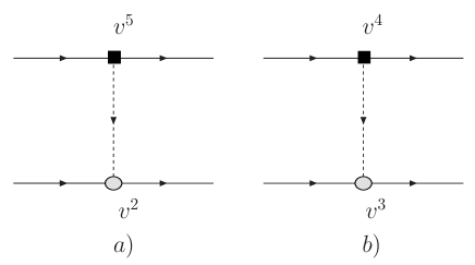
Figure 2: Leading order finite size spin²–spin contributions. The black square represents an insertion of the finite size operator

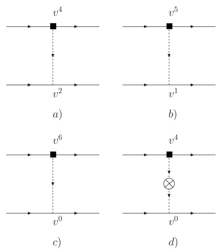
Figure 3: Diagrams contributing to the 3PN which do not involve non-linearities. The cross corresponds to a propagator correction, i.e. a retardation effect.

Fig. 3 shows 3PN contribution from one graviton exchange, with the last diagram corresponding to the first retardation effect, while Fig. 4 gives the contributions form non-linearities. Calculating these diagrams is straightforward. The results for each one of the diagrams are

$${}\mbox{Fig.~{}\ref{fs1n}a}=\frac{iC^{(1)}_{ES^{2}}3m_{2}}{4m_{1}}\frac{G_{N}}{r^{3}}~{}{\bf v}_{2}^{2}S_{1}^{ik}S_{1}^{jk}(3n^{i}n^{j}-\delta^{ij})$$ (41)

$${}\mbox{Fig.~{}\ref{fs1n}b}=-\frac{iC^{(1)}_{ES^{2}}m_{2}}{m_{1}}\frac{2G_{N}}{r^{3}}~{}{\bf v}_{2}\cdot{\bf v}_{1}S_{1}^{ik}S_{1}^{jk}(3n^{i}n^{j}-\delta^{ij}),$$

$${}\mbox{Fig.~{}\ref{fs1n}c}=-\frac{iC^{(1)}_{ES^{2}}m_{2}}{m_{1}}\frac{G_{N}}{2r^{3}}\left[S_{1}^{i0}S_{1}^{j0}(3n^{i}n^{j}-\delta^{ij})-2S_{1}^{0k}S_{1}^{jk}(v_{1}^{j}-3{\bf v}_{1}\cdot{\bf n}n^{j})\right.$$

$${}+\left.2S_{1}^{ik}S_{1}^{jk}\left((3{\bf n}\cdot{\bf v}_{1}n^{j}v_{1}^{i}-v_{1}^{i}v_{1}^{j})-\frac{3}{4}{\bf v}_{1}^{2}(3n^{i}n^{j}-\delta^{ij})+(v_{1}^{i}v_{2}^{j}-3{\bf v}_{2}\cdot{\bf n}n^{j}v_{1}^{i})-\frac{1}{2}\delta^{ij}{\bf a}_{1}\cdot{\bf r}\right)\right]$$

for the instantaneous one–graviton exchanges, and

$$\mbox{Fig~{}\ref{fs1n}d}=-iC^{(1)}_{ES^{2}}\frac{G_{N}m_{2}}{4m_{1}r^{3}}S_{1}^{ki}S_{1}^{kj}\left[{\bf v}_{1}\cdot{\bf v}_{2}(\delta^{ij}-3n^{i}n^{j})-3(v_{1}^{j}n^{i}+v_{1}^{i}n^{j}){\bf v}_{2}\cdot{\bf n}\right.$$

$$\left.-3{\bf v}_{1}\cdot{\bf n}(v_{2}^{j}n^{i}+v_{2}^{i}n^{j})+v_{1}^{i}v_{2}^{j}+v_{2}^{i}v_{1}^{j}-3{\bf v}_{1}\cdot{\bf n}{\bf v}_{2}\cdot{\bf n}(\delta^{ij}-5n^{i}n^{j})\right]$$ (42)

for the correction stemming from expanding the propagator.

For the non–linear terms, since the LO finite size insertion is proprtional to $H_{00,ij}$, we need the three point function $\langle H_{00}H_{00}H_{00}\rangle$, which we can get from the results for the spinless case in nrgr , and just correct for the worldline insertions. We end up with

$${}\mbox{Fig~{}\ref{fs2n}a}=-iC^{(1)}_{ES^{2}}\frac{G_{N}^{2}m^{2}_{2}}{m_{1}r^{4}}(4n_{i}n_{j}-\delta_{ij})S_{1}^{ik}S_{1}^{jk},$$ (43)

$${}\mbox{Fig~{}\ref{fs2n}b}=-iC^{(1)}_{ES^{2}}\frac{G_{N}^{2}m_{2}}{r^{4}}(3n_{i}n_{j}-\delta_{ij})S_{1}^{ik}S_{1}^{jk},$$ (44)

$${}\mbox{Fig~{}\ref{fs2n}c}=iC^{(1)}_{ES^{2}}\frac{G_{N}^{2}m_{2}}{2r^{4}}(3n_{i}n_{j}-\delta_{ij})S_{1}^{ik}S_{1}^{jk},$$ (45)

$${}\mbox{Fig~{}\ref{fs2n}d}=-iC^{(1)}_{ES^{2}}\frac{G_{N}^{2}m^{2}_{2}}{m_{1}r^{4}}(2n_{i}n_{j}-\delta_{ij})S_{1}^{ik}S_{1}^{jk}.$$ (46)

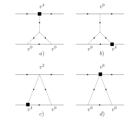
Figure 4: Non–linear finite size contributions to the 3PN spin–orbit potential.

As in ss , we split the potential at 3PN into two pieces

$$V^{s^{2}}_{S^{i0}} = C^{(1)}_{ES^{2}}\frac{G_{N}m_{2}}{2m_{1}r^{3}}\left[S_{1}^{j0}S_{1}^{i0}(3n^{i}n^{j}-\delta^{ij})-2S_{1}^{k0}\left(({\bf v}_{1}\times{\bf S}_{1})^{k}-3({\bf n}\cdot{\bf v}_{1})({\bf n}\times{\bf S}_{1})^{k}\right)\right]$$ (47)

$$+1\to 2$$

and

$$V^{s^{2}}_{\bf S} = C^{(1)}_{ES^{2}}\frac{G_{N}m_{2}}{2m_{1}r^{3}}\left[{\bf S}_{1}^{2}\left(6({\bf n}\cdot{\bf v}_{1})^{2}-\frac{15}{2}{\bf n}\cdot{\bf v}_{1}{\bf n}\cdot{\bf v}_{2}+\frac{13}{2}{\bf v}_{1}\cdot{\bf v}_{2}-\frac{3}{2}{\bf v}_{2}^{2}-\frac{7}{2}{\bf v}_{1}^{2}-2{\bf a}_{1}\cdot{\bf r}\right)\right.$$ (48)

$$+ ({\bf S}_{1}\cdot{\bf n})^{2}\left(\frac{9}{2}({\bf v}_{1}^{2}+{\bf v}_{2}^{2})-\frac{21}{2}{\bf v}_{1}\cdot{\bf v}_{2}-\frac{15}{2}{\bf n}\cdot{\bf v}_{1}{\bf n}\cdot{\bf v}_{2}\right)+2{\bf v}_{1}\cdot{\bf S}_{1}{\bf v}_{1}\cdot{\bf S}_{1}$$

$$- \left.3{\bf v}_{1}\cdot{\bf S}_{1}{\bf v}_{2}\cdot{\bf S}_{1}-6{\bf n}\cdot{\bf v}_{1}{\bf n}\cdot{\bf S}_{1}{\bf v}_{1}\cdot{\bf S}_{1}+9{\bf n}\cdot{\bf v}_{2}{\bf n}\cdot{\bf S}_{1}{\bf v}_{1}\cdot{\bf S}_{1}+3{\bf n}\cdot{\bf v}_{1}{\bf n}\cdot{\bf S}_{1}{\bf v}_{2}\cdot{\bf S}_{1}\right]$$

$$+C^{(1)}_{ES^{2}}\frac{m_{2}G_{N}^{2}}{2r^{4}}\left(1+\frac{4m_{2}}{m_{1}}\right)\left({\bf S}_{1}^{2}-3({\bf S}_{1}\cdot{\bf n})^{2}\right)+1\to 2.$$

III.5 The $S^{2}$ potential in the covariant SSC

Collecting all the pieces together we end up with the following expression for the spin² potential to 3PN in the covariant SSC

$$V_{3PN}^{s^{2}} = V^{RS^{2}}_{3PN}+V^{s^{2}}_{S^{0i}}+V^{s^{2}}_{\bf S}+V^{s^{2}}_{nl}+V^{s^{2}}_{2PN}$$

$$= C^{(1)}_{ES^{2}}\frac{G_{N}m_{2}}{2m_{1}r^{3}}\left[S_{1}^{j0}S_{1}^{i0}(3n^{i}n^{j}-\delta^{ij})-2S_{1}^{k0}\left(({\bf v}_{1}\times{\bf S}_{1})^{k}-3({\bf n}\cdot{\bf v}_{1})({\bf n}\times{\bf S}_{1})^{k}\right)\right]$$

$$+C^{(1)}_{ES^{2}}\frac{G_{N}m_{2}}{2m_{1}r^{3}}\left[{\bf S}_{1}^{2}\left(6({\bf n}\cdot{\bf v}_{1})^{2}-\frac{15}{2}{\bf n}\cdot{\bf v}_{1}{\bf n}\cdot{\bf v}_{2}+\frac{13}{2}{\bf v}_{1}\cdot{\bf v}_{2}-\frac{3}{2}{\bf v}_{2}^{2}-\frac{7}{2}{\bf v}_{1}^{2}-2{\bf a}_{1}\cdot{\bf r}\right)\right.$$

$$+({\bf S}_{1}\cdot{\bf n})^{2}\left(\frac{9}{2}({\bf v}_{1}^{2}+{\bf v}_{2}^{2})-\frac{21}{2}{\bf v}_{1}\cdot{\bf v}_{2}-\frac{15}{2}{\bf n}\cdot{\bf v}_{1}{\bf n}\cdot{\bf v}_{2}\right)+2{\bf v}_{1}\cdot{\bf S}_{1}{\bf v}_{1}\cdot{\bf S}_{1}$$

$$-\left.3{\bf v}_{1}\cdot{\bf S}_{1}{\bf v}_{2}\cdot{\bf S}_{1}-6{\bf n}\cdot{\bf v}_{1}{\bf n}\cdot{\bf S}_{1}{\bf v}_{1}\cdot{\bf S}_{1}+9{\bf n}\cdot{\bf v}_{2}{\bf n}\cdot{\bf S}_{1}{\bf v}_{1}\cdot{\bf S}_{1}+3{\bf n}\cdot{\bf v}_{1}{\bf n}\cdot{\bf S}_{1}{\bf v}_{2}\cdot{\bf S}_{1}\right]$$

$$-C^{(1)}_{ES^{2}}\frac{m_{2}G_{N}}{2m_{1}r^{3}}\left({\bf S}_{1}^{2}-3({\bf S}_{1}\cdot{\bf n})^{2}\right)+C^{(1)}_{ES^{2}}\frac{m_{2}G_{N}^{2}}{2r^{4}}\left(1+\frac{4m_{2}}{m_{1}}\right)\left({\bf S}_{1}^{2}-3({\bf S}_{1}\cdot{\bf n})^{2}\right)$$

$$-\frac{G_{N}^{2}m_{2}}{r^{4}}\left({\bf S}_{1}\cdot{\bf n}\right)^{2}+\left({\bf\tilde{a}}^{so}_{1(1)}\right)^{l}S_{1}^{0l}+{\bf v}_{1}\times{\bf S}_{1}\cdot{\bf\tilde{a}}^{so}_{1(1)}+1\leftrightarrow 2.$$

In appendix B we provide a cross check for this potential by taking the extreme mass ratio limit and showing that we reproduce the motion of a test particle in a Kerr background as expected.

III.6 Divergences and Regularization

In computing the Feynman diagrams leading to the expression in (III.5) we encounter divergences of many sorts. First of all from Wick contractions such as the ones represented in Fig. 5.

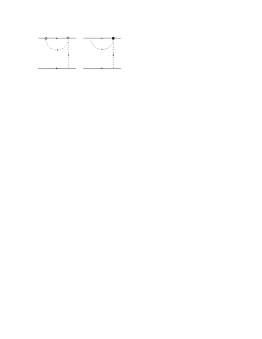
Figure 5: Divergent diagrams which renormalize the mass and quadrupole couplings.

These diagrams however simply renormalize the couplings of our theory, $m_{q}$ and $C^{(q)}_{ES^{2}}$ coefficients. The divergences are power like and are thus ”pure counter–terms” (see TASI for a discussion for non-experts). Thus, no renormalization group (RG) flow is present in this case, contrary to the case of logarithmic divergences nrgr ; nrgr3 ; ss . In the case of dimensional regularization, these diagrams are automatically set to zero since they involve scaleless integrals. Other divergences are found for instance in diagrams such as Fig. 4ab, or similarly in Fig. 1. These divergences occur when a factor of momentum squared in the numerator from the three graviton vertex cancels the intermediate propagator line connecting with the external worldline. Effectively the resulting diagrams appears as in Fig 5. These represent a (pure counterterm) renormalization of the mass and the finite size coefficient $C_{ES^{2}}$.

At higher order, tidally induced logarithmic divergences will appear. As shown in nrgr3 , the first tidally induced finite size effects starts out at 5PN for maximally rotating compact objects, from a higher dimensional operators of the form

$$C_{D^{2}ES^{2}}(\mu)D^{2}E_{ab}S^{a}_{c}S^{cb}.$$ (50)

In the expression of (50) $C_{D^{2}ES^{2}}(\mu)$ is a Wilson coefficients which obeys a RG–type of equation,

$$\mu\frac{d}{d\mu}C_{D^{2}ES^{2}}(\mu)\sim\frac{m}{m_{p}^{4}}.$$ (51)

Notice that (50) does not contribute to the one–point function, as it is expected from Birkoff’s theorem. That is due to the fact that $D^{2}h_{\mu\nu}\sim{\cal O}(h^{2})$ on shell, and the linear piece in (50) can be traded, by a field redefinition, for a term proportional to $h^{2}$. Therefore, (50) does contribute to the (n+1)–point function and that is how we can match with the full theory using scattering amplitudes. This result generalizes the effacement of internal structure up to 5PN order, modulo self–induced effects computed in this paper, to the case of spinning bodies.

IV The S² contribution to the spin dynamics to 3PN in the covariant SSC

From (III.5) we can obtain the spin dynamics using (2). The result reads

$$\frac{d{\bf S}_{1}}{dt}=(\omega_{s^{2}}^{2PN}+{\omega}^{3PN}_{s^{2}})\times{\bf S}_{1}+({\bf\tilde{a}}^{so}_{1(1)}\times{\bf S}_{1})\times{\bf v}_{1}+({\bf v}_{1}\times{\bf S}_{1})\times{\bf A}_{1}+{\bf B}_{1}\times{\bf S}_{1}$$ (52)

where we included the term from the Routhian in (30), and

$$\omega_{2PN}^{s^{2}}=3C^{(1)}_{ES^{2}}\frac{m_{2}G_{N}}{m_{1}r^{3}}{\bf n}({\bf S}_{1}\cdot{\bf n}).$$ (53)

Also

$${\bf A}_{1}={\bf v}_{1}\times\omega_{2PN}^{s^{2}},$$ (54)

and

$${\bf B}_{1}=\frac{C^{(1)}_{ES^{2}}m_{2}}{2m_{1}r^{3}}\left[2{\bf v}_{1}({\bf S}_{1}\cdot{\bf v}_{1})-6{\bf v}_{1}({\bf n}\cdot{\bf v}_{1})({\bf S}_{1}\cdot{\bf n})\right],$$ (55)

$${\omega}_{3PN}^{s^{2}} = C^{(1)}_{ES^{2}}\frac{G_{N}m_{2}}{2m_{1}r^{3}}\left[2({\bf S}_{1}\cdot{\bf n}){\bf n}\left(\frac{9}{2}({\bf v}_{1}^{2}+{\bf v}_{2}^{2})-\frac{21}{2}{\bf v}_{1}\cdot{\bf v}_{2}-\frac{15}{2}{\bf n}\cdot{\bf v}_{1}{\bf n}\cdot{\bf v}_{2}\right)+4{\bf v}_{1}({\bf v}_{1}\cdot{\bf S}_{1})\right.$$ (56)

$$- \left.3{\bf v}_{1}({\bf v}_{2}\cdot{\bf S}_{1})-3{\bf v}_{2}({\bf v}_{1}\cdot{\bf S}_{1})-6{\bf n}({\bf n}\cdot{\bf v}_{1})({\bf v}_{1}\cdot{\bf S}_{1})-6{\bf v}_{1}({\bf n}\cdot{\bf v}_{1})({\bf n}\cdot{\bf S}_{1})\right.$$

$$+ \left.9{\bf n}({\bf n}\cdot{\bf v}_{2})({\bf v}_{1}\cdot{\bf S}_{1})+9{\bf v}_{1}({\bf n}\cdot{\bf v}_{2})({\bf n}\cdot{\bf S}_{1})+3{\bf n}({\bf n}\cdot{\bf v}_{1})({\bf v}_{2}\cdot{\bf S}_{1})\right.$$

$$+ \left.3{\bf v_{2}}({\bf n}\cdot{\bf v}_{1})({\bf n}\cdot{\bf S}_{1})\right]-C^{(1)}_{ES^{2}}\frac{m_{2}G_{N}^{2}}{r^{4}}\left(1+\frac{4m_{2}}{m_{1}}\right)3{\bf n}({\bf S}_{1}\cdot{\bf n})-\frac{2m_{2}G_{N}^{2}}{r^{4}}{\bf n}({\bf S}_{1}\cdot{\bf n}).$$

IV.1 The precession equation

The spin EOM in (52) can be transformed into a precession form by performing the transformation to the NW SSC which we applied in ss

$${\bf S}^{nw}_{1}=\left(1-\frac{1}{2}{\bf\tilde{v}}_{1}^{2}\right){\bf S}_{1}+\frac{1}{2}{\bf\tilde{v}}_{1}({\bf\tilde{v}}_{1}\cdot{\bf S}_{1})+\frac{G_{N}}{2r^{2}}\left[({\bf n}\times{\bf S}_{2})\times{\bf v}_{2}\right]\times{\bf S}_{1}+\ldots$$ (57)

with $\bf\tilde{v}$ the velocity in the local frame given by

$${\bf\tilde{v}}_{1}=\left(1+\frac{G_{N}m_{2}}{r}\right){\bf v}_{1}+\frac{G_{N}}{r^{2}}{\bf n}\times{\bf S}_{2}+\ldots$$ (58)

and

$${\bf x}_{q}\to{\bf x}_{q}-\frac{1}{2m_{q}}({\bf v}_{q}\times{\bf S}_{q})+\ldots,$$ (59)

where the ellipses represent higher order corrections.

The EOM in terms of ${\bf S}^{nw}$ takes a precession form. This form was already shown for the ${\bf S}^{nw}_{1}{\bf S}^{nw}_{2}$ sector ss , and now for ${\left({\bf S}^{nw}_{1}\right)}^{2}$ effects we have

$$\frac{d}{dt}{\bf S}_{1}^{nw}=\omega^{nw}_{s^{2}}\times{\bf S}^{nw}_{1}$$ (60)

with (we suppressed the $nw$ label in the spin vector for simplicity)

$$\omega^{nw}_{s^{2}}=\omega_{s^{2}}^{2PN}+{\omega}^{3PN}_{s^{2}}+{\bf B}_{1}+\frac{1}{2}\left({\bf\tilde{a}}_{1(1)}+\omega_{s^{2}}^{2PN}\times{\bf v}_{1}\right)\times{\bf v}_{1}+\delta\omega^{s^{2}}_{so}+\delta\omega^{2PN}_{s^{2}}$$ (61)

where ${\bf\tilde{a}}_{1(1)}$ and ${\bf B}_{1}$ are given by (29) and (55) respectively. We also have the ${\cal O}({\bf S}_{1})$ pieces of the shift in the spin–orbit frequency after (57) (which effectively takes the covariant result into the NW spin–orbit precession as shown in ss ) and hence from (59) (see also eq. (74) in ss ),

$$\delta\omega^{s^{2}}_{so} = \frac{m_{2}G_{N}}{2m_{1}r^{3}}\left\{{\bf n}\times\left(\frac{9}{2}{\bf v}_{1}-6{\bf v}_{2}\right)({\bf n}\times{\bf v}_{1})\cdot{\bf S}_{1}+{\bf v}_{1}{\bf S}_{1}\cdot\left(\frac{3}{2}{\bf v}_{1}-2{\bf v}_{2}\right)\right\}$$ (62)

$$+\frac{3}{4}\frac{G_{N}^{2}m_{2}^{2}}{m_{1}r^{4}}{\bf n}({\bf n}\cdot{\bf S}_{1}).$$

Also from the inverse of (57) in the LO finite size term

$$\delta\omega^{2PN}_{s^{2}}=C_{ES^{2}}^{(1)}\frac{3G_{N}m_{2}}{2m_{1}r^{3}}\left[{\bf n}({\bf n}\cdot{\bf S}_{1}){\bf v}_{1}^{2}-{\bf n}({\bf n}\cdot{\bf v}_{1})({\bf v}_{1}\cdot{\bf S}_{1})\right].$$ (63)

V The spin potential to 3PN in the covariant SSC

For completeness here we re–write the spin–spin and spin² potentials, including also the LO spin–orbit term,

$$V^{spin} = \frac{G_{N}m_{2}}{r^{2}}n^{j}\left(S^{j0}_{1}+S^{jk}_{1}(v_{1}^{k}-2v^{k}_{2})\right)-\frac{G_{N}m_{1}}{r^{2}}n^{j}\left(S^{j0}_{2}+S^{jk}_{2}(v_{2}^{k}-2v^{k}_{1})\right)$$

$$-\frac{G_{N}}{r^{3}}\left[(\delta^{ij}-3n^{i}n^{j})\left(S^{i0}_{1}S^{j0}_{2}+\frac{1}{2}{\bf v}_{1}\cdot{\bf v}_{2}S^{ik}_{1}S^{jk}_{2}+v_{1}^{m}v_{2}^{k}S^{ik}_{1}S^{jm}_{2}-v_{1}^{k}v_{2}^{m}S^{ik}_{1}S^{jm}_{2}\right.\right.$$

$$+\left.S^{i0}_{1}S^{jk}_{2}(v_{2}^{k}-v_{1}^{k})+S^{ik}_{1}S^{j0}_{2}(v_{1}^{k}-v_{2}^{k})\right)+\frac{1}{2}S_{1}^{ki}S_{2}^{kj}\left(3{\bf v}_{1}\cdot{\bf n}{\bf v}_{2}\cdot{\bf n}(\delta^{ij}-5n^{i}n^{j})\right.$$

$$+\left.3{\bf v}_{1}\cdot{\bf n}(v_{2}^{j}n^{i}+v_{2}^{i}n^{j})+3{\bf v}_{2}\cdot{\bf n}(v_{1}^{j}n^{i}+v_{1}^{i}n^{j})-v_{1}^{i}v_{2}^{j}-v_{2}^{i}v_{1}^{j}\right)$$

$$+\left.(3n^{l}{\bf v}_{2}\cdot{\bf n}-v_{2}^{l})S_{1}^{0k}S_{2}^{kl}+(3n^{l}{\bf v}_{1}\cdot{\bf n}-v_{1}^{l})S_{2}^{0k}S_{1}^{kl}\right]$$

$$+\left(\frac{G_{N}}{r^{3}}-\frac{3MG_{N}^{2}}{r^{4}}\right)S_{1}^{jk}S_{2}^{ji}(\delta^{ki}-3n^{k}n^{i})$$

$$+\left\{C^{(1)}_{ES^{2}}\frac{G_{N}m_{2}}{2m_{1}r^{3}}\left[S_{1}^{j0}S_{1}^{i0}(3n^{i}n^{j}-\delta^{ij})-2S_{1}^{k0}\left(({\bf v}_{1}\times{\bf S}_{1})^{k}-3({\bf n}\cdot{\bf v}_{1})({\bf n}\times{\bf S}_{1})^{k}\right)\right]\right.$$

$$+C^{(1)}_{ES^{2}}\frac{G_{N}m_{2}}{2m_{1}r^{3}}\left[{\bf S}_{1}^{2}\left(6({\bf n}\cdot{\bf v}_{1})^{2}-\frac{15}{2}{\bf n}\cdot{\bf v}_{1}{\bf n}\cdot{\bf v}_{2}+\frac{13}{2}{\bf v}_{1}\cdot{\bf v}_{2}-\frac{3}{2}{\bf v}_{2}^{2}-\frac{7}{2}{\bf v}_{1}^{2}-2{\bf a}_{1}\cdot{\bf r}\right)\right.$$

$$+({\bf S}_{1}\cdot{\bf n})^{2}\left(\frac{9}{2}({\bf v}_{1}^{2}+{\bf v}_{2}^{2})-\frac{21}{2}{\bf v}_{1}\cdot{\bf v}_{2}-\frac{15}{2}{\bf n}\cdot{\bf v}_{1}{\bf n}\cdot{\bf v}_{2}\right)+2{\bf v}_{1}\cdot{\bf S}_{1}{\bf v}_{1}\cdot{\bf S}_{1}$$

$$-\left.3{\bf v}_{1}\cdot{\bf S}_{1}{\bf v}_{2}\cdot{\bf S}_{1}-6{\bf n}\cdot{\bf v}_{1}{\bf n}\cdot{\bf S}_{1}{\bf v}_{1}\cdot{\bf S}_{1}+9{\bf n}\cdot{\bf v}_{2}{\bf n}\cdot{\bf S}_{1}{\bf v}_{1}\cdot{\bf S}_{1}+3{\bf n}\cdot{\bf v}_{1}{\bf n}\cdot{\bf S}_{1}{\bf v}_{2}\cdot{\bf S}_{1}\right]$$

$$-C^{(1)}_{ES^{2}}\frac{m_{2}G_{N}}{2m_{1}r^{3}}\left({\bf S}_{1}^{2}-3({\bf S}_{1}\cdot{\bf n})^{2}\right)+C^{(1)}_{ES^{2}}\frac{m_{2}G_{N}^{2}}{2r^{4}}\left(1+\frac{4m_{2}}{m_{1}}\right)\left({\bf S}_{1}^{2}-3({\bf S}_{1}\cdot{\bf n})^{2}\right)$$

$$\left.-\frac{G_{N}^{2}m_{2}}{r^{4}}\left({\bf S}_{1}\cdot{\bf n}\right)^{2}+\left({\bf\tilde{a}}^{so}_{1(1)}\right)^{l}S_{1}^{0l}+{\bf v}_{1}\times{\bf S}_{1}\cdot{\bf\tilde{a}}^{so}_{1(1)}+1\leftrightarrow 2\right\},$$

which allows us to obtain the ${\cal O}({\bf S}_{1}{\bf S}_{2})$ (computed in ss ) and ${\cal O}({\bf S}_{1(2)}^{2})$ contributions to the EOM to 3PN in the covariant SSC. The latter is imposed after the EOM are obtained via (2). Note that, to the order we are working in this paper, we can replace the acceleration-dependent term in our Lagrangian by the LO equations of motion, or equivalently integrate it by parts.

Missing in (V) is the NLO spin–orbit potential. The latter was obtained in owen ; buon . However, recall that our computation is in terms of the spin in the local frame, $S^{ab}$, whereas in owen ; buon the spin dynamics was calculated in terms of the spin tensor in the PN frame. e.g. $S^{\mu\nu}$. The result can be translated to the local frame by using the tetrad field $e^{a}_{\mu}$ ss . The potential in (V) therefore completes the computation of spin effects to 3PN.

VI conclusions

In this paper we have completed the calculation of the potential quadratic in spins to 3PN. Together with our previous results in eih ; comment ; ss , the results in this paper complete the computation of the relevant potentials to obtain the spin effects in the EOM to 3PN order. It is important to note that within NRGR there is no obstacle to go beyond this order using the formalism developed in nrgr ; ss . In particular, the NNLO corrections should follow with relative ease. The radiation at 3PN from spinning binaries remains to be calculated. The framework for such a calculation within NRGR was set up in nrgr . We report on these effects in radss .

Appendix A Using ${\cal S}$ instead of $S$

In this appendix we compute the subleading finite size corrections using (15), which we will explicitly show give rise to identical results to those found in the body of the paper. The calculation is identical, the only exception is that now we use ${\cal S}^{ab}$ in the diagrams. As we did in ss , we can sum up all the diagrams and hence split the finite size potential at 3PN in two pieces, as we did before in (48) and (47). Hence we have again one term dependent on ${\cal S}^{i0}$,

$$V^{s^{2}}_{{\cal S}^{i0}} = C^{(1)}_{ES^{2}}\frac{G_{N}m_{2}}{2m_{1}r^{3}}\left[{\cal S}_{1}^{j0}{\cal S}_{1}^{i0}(3n^{i}n^{j}-\delta^{ij})-2{\cal S}_{1}^{k0}\left(({\bf v}_{1}\times{\bf S}_{1})^{k}-3({\bf n}\cdot{\bf v}_{1})({\bf n}\times{\bf S}_{1})^{k}\right)\right]+1\to 2$$ (65)

$$= C^{(1)}_{ES^{2}}\frac{G_{N}m_{2}}{2m_{1}r^{3}}\left[-3({\bf v}_{1}\times{\bf S}_{1})^{2}+3\left({\bf n}\cdot({\bf v}_{1}\times{\bf S}_{1})\right)^{2}+6({\bf n}\cdot{\bf v}_{1})({\bf v}_{1}\times{\bf S}_{1})\cdot({\bf n}\times{\bf S}_{1})\right]$$

$$+1\to 2$$

where we used (10), and as before at 3PN,

$$V^{s^{2}}_{\bf S} = C^{(1)}_{ES^{2}}\frac{G_{N}m_{2}}{2m_{1}r^{3}}\left[{\bf S}_{1}^{2}\left(6({\bf n}\cdot{\bf v}_{1})^{2}-\frac{15}{2}{\bf n}\cdot{\bf v}_{1}{\bf n}\cdot{\bf v}_{2}-\frac{13}{2}{\bf v}_{1}\cdot{\bf v}_{2}-\frac{3}{2}{\bf v}_{2}^{2}-\frac{7}{2}{\bf v}_{1}^{2}-2{\bf a}_{1}\cdot{\bf r}\right)\right.$$ (66)

$$+ ({\bf S}_{1}\cdot{\bf n})^{2}\left(\frac{9}{2}({\bf v}_{1}^{2}+{\bf v}_{2}^{2})-\frac{21}{2}{\bf v}_{1}\cdot{\bf v}_{2}-\frac{15}{2}{\bf n}\cdot{\bf v}_{1}{\bf n}\cdot{\bf v}_{2}\right)+2{\bf v}_{1}\cdot{\bf S}_{1}{\bf v}_{1}\cdot{\bf S}_{1}$$

$$- \left.3{\bf v}_{1}\cdot{\bf S}_{1}{\bf v}_{2}\cdot{\bf S}_{1}-6{\bf n}\cdot{\bf v}_{1}{\bf n}\cdot{\bf S}_{1}{\bf v}_{1}\cdot{\bf S}_{1}+9{\bf n}\cdot{\bf v}_{2}{\bf n}\cdot{\bf S}_{1}{\bf v}_{1}\cdot{\bf S}_{1}+3{\bf n}\cdot{\bf v}_{1}{\bf n}\cdot{\bf S}_{1}{\bf v}_{2}\cdot{\bf S}_{1}\right]$$

$$+C^{(1)}_{ES^{2}}\frac{m_{2}G_{N}^{2}}{2r^{4}}\left(1+\frac{4m_{2}}{m_{1}}\right)\left({\bf S}_{1}^{2}-3({\bf S}_{1}\cdot{\bf n})^{2}\right)+1\to 2.$$

We are still one term short to complete the potential to 3PN. We still need to include the subleading corrections due to (9) in the LO finite size potential of (17),

$$V^{s^{2}}_{2PN}\to C^{(1)}_{ES^{2}}\frac{m_{2}G_{N}}{2m_{1}r^{3}}{\cal S}_{1}^{ik}{\cal S}_{1}^{jk}(\delta^{ij}-3n^{i}n^{j})+1\to 2.$$ (67)

Equivalently we have

$$V^{s^{2}}_{2PN}\to-C^{(1)}_{ES^{2}}\frac{m_{2}G_{N}}{2m_{1}r^{3}}\left({\bf\cal S}_{1}\cdot{\bf\cal S}_{1}-3{\bf\cal S}_{1}\cdot{\bf n}{\bf\cal S}_{1}\cdot{\bf n}\right)+1\to 2,$$ (68)

with ${\bf\cal S}_{q}^{ij}=\epsilon^{ijk}{\cal S}^{k}$, and

$$\{S^{i}_{q},{\cal S}_{q}^{k}\}=-\epsilon^{ikl}(S_{q}^{l}+({\bf S}_{q}\cdot{\bf v}_{q})v_{q}^{l}).$$ (69)

The final result for the spin² potential in the covariant SSC turns out to be the sum of each previous computations in (28), (22), (47), (48) and (68), resulting in

$$V_{3PN}^{s^{2}} = V^{RS^{2}}_{3PN}+V^{s^{2}}_{{\cal S}^{0i}}+V^{s^{2}}_{\bf S}+V^{s^{2}}_{nl}+V^{s^{2}}_{2PN}({\bf\cal S})$$

$$= C^{(1)}_{ES^{2}}\frac{G_{N}m_{2}}{2m_{1}r^{3}}\left[-3({\bf v}_{1}\times{\bf S}_{1})^{2}+3\left({\bf n}\cdot({\bf v}_{1}\times{\bf S}_{1})\right)^{2}+6({\bf n}\cdot{\bf v}_{1})({\bf v}_{1}\times{\bf S}_{1})\cdot({\bf n}\times{\bf S}_{1})\right]$$

$$+ C^{(1)}_{ES^{2}}\frac{G_{N}m_{2}}{2m_{1}r^{3}}\left[{\bf S}_{1}^{2}\left(6({\bf n}\cdot{\bf v}_{1})^{2}-\frac{15}{2}{\bf n}\cdot{\bf v}_{1}{\bf n}\cdot{\bf v}_{2}+\frac{13}{2}{\bf v}_{1}\cdot{\bf v}_{2}-\frac{3}{2}{\bf v}_{2}^{2}-\frac{7}{2}{\bf v}_{1}^{2}-2{\bf a}_{1}\cdot{\bf r}\right)\right.$$

$$+ ({\bf S}_{1}\cdot{\bf n})^{2}\left(\frac{9}{2}({\bf v}_{1}^{2}+{\bf v}_{2}^{2})-\frac{21}{2}{\bf v}_{1}\cdot{\bf v}_{2}-\frac{15}{2}{\bf n}\cdot{\bf v}_{1}{\bf n}\cdot{\bf v}_{2}\right)+2{\bf v}_{1}\cdot{\bf S}_{1}{\bf v}_{1}\cdot{\bf S}_{1}$$

$$- \left.3{\bf v}_{1}\cdot{\bf S}_{1}{\bf v}_{2}\cdot{\bf S}_{1}-6{\bf n}\cdot{\bf v}_{1}{\bf n}\cdot{\bf S}_{1}{\bf v}_{1}\cdot{\bf S}_{1}+9{\bf n}\cdot{\bf v}_{2}{\bf n}\cdot{\bf S}_{1}{\bf v}_{1}\cdot{\bf S}_{1}+3{\bf n}\cdot{\bf v}_{1}{\bf n}\cdot{\bf S}_{1}{\bf v}_{2}\cdot{\bf S}_{1}\right]$$

$$+ C^{(1)}_{ES^{2}}\frac{m_{2}G_{N}^{2}}{2r^{4}}\left(1+\frac{4m_{2}}{m_{1}}\right)\left({\bf S}_{1}^{2}-3({\bf S}_{1}\cdot{\bf n})^{2}\right)-\frac{G_{N}^{2}m_{2}}{r^{4}}\left({\bf S}_{1}\cdot{\bf n}\right)^{2}$$

$$- C^{(1)}_{ES^{2}}\frac{m_{2}G_{N}}{2m_{1}r^{3}}\left({\bf\cal S}_{1}\cdot{\bf\cal S}_{1}-3{\bf\cal S}_{1}\cdot{\bf n}{\bf\cal S}_{1}\cdot{\bf n}\right)+\left({\bf\tilde{a}}^{so}_{1(1)}\right)^{l}S_{1}^{0l}+{\bf v}_{1}\times{\bf S}_{1}\cdot{\bf\tilde{a}}^{so}_{1(1)}+1\to 2,$$

where ${\bf\tilde{a}}^{so}_{1(1)}$ is given by (29) and ${\cal S}^{i}=\frac{1}{2}\epsilon^{ijk}{\cal S}^{jk}$, with ${\cal S}^{jk}$ given in (11). with the algebra in (69) for the ${\bf\cal S}$ pieces. The squared spin contribution to the EOM in the covariant SSC thus read

$$\frac{d{\bf S}_{1}}{dt} = (\omega_{s^{2}}^{2PN}+{\hat{\omega}}^{3PN}_{s^{2}})\times{\bf S}_{1}+({\bf\tilde{a}}^{so}_{1(1)}\times{\bf S}_{1})\times{\bf v}_{1}+({\bf S}_{1}\cdot{\bf v}_{1})\omega^{2PN}_{s^{2}}\times{\bf v}_{1},$$ (71)

where again

$$\omega_{2PN}^{s^{2}}=3C^{(1)}_{ES^{2}}\frac{m_{2}G_{N}}{m_{1}r^{3}}{\bf n}({\bf S}_{1}\cdot{\bf n}),$$ (72)

and

$${\hat{\omega}}_{3PN}^{s^{2}} = {\bar{\omega}}_{3PN}^{s^{2}}+{\omega}_{3PN}^{s^{2}}$$ (73)

$${\bar{\omega}}_{3PN}^{s^{2}} = 3C^{(1)}_{ES^{2}}\frac{G_{N}m_{2}}{m_{1}r^{3}}\left[{\bf v}_{1}({\bf v}_{1}\cdot{\bf S}_{1})+{\bf n}\times{\bf v}_{1}\left({\bf n}\cdot({\bf v}_{1}\times{\bf S}_{1})\right)\right.$$

$$\left.-{\bf n}({\bf n}\cdot{\bf v}_{1})({\bf S}_{1}\cdot{\bf v}_{1})-{\bf v}_{1}({\bf n}\cdot{\bf v}_{1})({\bf S}_{1}\cdot{\bf n})\right]$$

with ${\omega}^{s^{2}}_{3PN}$ given in (56). We can now compare the expression in (52) with (71) and (73). Using

$$\left({\bf B}_{1}+(\omega^{s^{2}}_{2PN}\times{\bf v}_{1})\times{\bf v}_{1}\right)\times{\bf S}_{1}={\bar{\omega}}^{s^{2}}_{3PN}\times{\bf S}_{1}=-3C^{(1)}_{ES^{2}}\frac{G_{N}m_{2}}{m_{1}r^{3}}{\bf v}_{1}^{2}({\bf n\cdot S}_{1})({\bf n\times S}_{1})$$ (75)

one can show both spin EOM are indeed identical and the equivalence is thus proven.

Appendix B Checking the extreme mass ratio limit

In this appendix we compare our results to the extremal limit. That is, we consider the motion of a test particle with mass $m$ and velocity ${\bf v}$, moving in the background of a spinning BH with mass $M$ and spin ${\bf S}$. In this limit the potential is given by (recall $C_{ES^{2}}=1$ for a Kerr BH)

$$V_{stat} = -\frac{G_{N}m}{2Mr^{3}}({\bf S}^{2}-3({\bf S}\cdot{\bf n})^{2})+\frac{G_{N}^{2}m}{2r^{4}}({\bf S}^{2}-3({\bf n}\cdot{\bf S})^{2})-\frac{G_{N}^{2}m}{r^{4}}({\bf S}\cdot{\bf n})^{2}$$ (76)

$$-\frac{3G_{N}m}{4Mr^{3}}{\bf v}^{2}({\bf S}^{2}-3({\bf S}\cdot{\bf n})^{2}),$$

where we neglect term of order ${\cal O}(m^{2})$ (including the acceleration-dependent part of our potential).

Now we would like to compare this to the effective action generated via

$$S=-m\int dt\sqrt{g_{\mu\nu}\frac{dx^{\mu}}{dt}\frac{dx^{\nu}}{dt}}$$ (77)

by using the harmonic gauge metric hergt

$$ds^{2}=g_{00}dt^{2}+2g_{0\phi}dtd\phi+dl_{a}^{2}+dl_{a^{2}}^{2}$$ (78)

where the relevant pieces are (with signature $(-1,1,1,1)$)

$$g_{00} = -1+\frac{2G_{N}M}{r}-\frac{2G_{N}^{2}M^{2}}{r^{2}}-\frac{G_{N}S^{2}/M-4G_{N}^{3}M^{3}+3G_{N}S^{2}/M\cos(2\theta)}{2r^{3}}$$

$$+\frac{2G_{N}^{2}S^{2}-2G_{N}^{4}M^{4}+4G_{N}^{2}S^{2}\cos(2\theta)}{r^{4}}$$

$$g_{0\phi} = -\frac{2SG_{N}\sin^{2}\theta}{r}+\frac{2SMG_{N}^{2}\sin^{2}\theta}{r^{2}}+O(G_{N}^{3},S^{3})$$ (79)

$$dl_{a^{2}}^{2}=\frac{G_{N}S^{2}}{2Mr}\sin^{2}\theta\left(-(1+3\cos(2\theta))+\frac{G_{N}M(\cos(2\theta)-3)}{r}\right)d\phi^{2}$$ (80)

$$dl_{a}^{2}=((r+G_{N}M)^{2}\sin^{2}\theta+O(G_{N}S))d\phi^{2}.$$ (81)

For simplicity of comparison, and with no loss of generality, we consider the motion in a circular orbit. Notice that we do not expect our results to agree with those in the harmonic gauge to all orders in $G_{N}$, since we are working in a “background field harmonic” gauge. However, one can show that the coordinate transformation to the harmonic gauge will have no effect to the order we are working in this paper. Indeed plugging in (B) into (77) (after changing to our signature convention $(1,-1,-1,-1)$) and expanding leads to the result in (76).

References

- (1) R. A. Porto and I.Z. Rothstein, Phys.Rev.Lett. 97, 021101 (2006)
- (2) R. A. Porto and I. Z. Rothstein, “Comment on ‘On the next-to-leading order gravitational spin(1)-spin(2) dynamics’ by J. Steinhoff et al,” arXiv:0712.2032 [gr-qc].
- (3) R. A. Porto, “New results at 3PN via an effective field theory of gravity”. Proceedings of the 11th Marcel Grossmann Meeting on Recent Developments in Theoretical and Experimental General Relativity, Gravitation, and Relativistic Field Theories, arXiv:gr-qc/0701106.
- (4) W. Goldberger and I. Rothstein, Phys. Rev. D 73, 104029 (2006)
- (5) W. D. Goldberger and I. Z. Rothstein, Gen. Rel. Grav. 38, 1537 (2006) [Int. J. Mod. Phys. D 15, 2293 (2006)]
- (6) W. Goldberger and I. Rothstein, Phys. Rev. D 73, 104030 (2006)
- (7) R. A. Porto, Phys.Rev. D 73, 104031 (2006)
- (8) For a review see W. Goldberger “Les Houches lectures on effective field theories and gravitational radiation.” Proceedings of Les Houches summer school - Session 86: Particle Physics and Cosmology: The Fabric of Spacetime, arXiv: hep-ph/0701129. Also, R. A. Porto and R. Sturani, “Scalar gravity: Post-Newtonian corrections via an effective field theory approach” Ibidem, arXiv: gr-qc/0701105.
- (9) R. A. Porto, “Absorption Effects due to Spin in the Worldline Approach to Black Hole Dynamics,” arXiv:0710.5150 [hep-th] to appear in Phys. Rev. D.
- (10) See A. K. Leibovich contribution in workshop .
- (11) C. R. Galley and B. L. Hu, “Self-force on extreme mass ratio inspirals via curved spacetime effective field theory,” arXiv:0801.0900 [gr-qc].
- (12) K. Yee and M. Bander, Phys. Rev. D 48, 2797 (1993)
- (13) R. A. Porto and I. Z. Rothstein, “Spin(1)Spin(2) Effects in the Motion of Inspiralling Compact Binaries at Third Order in the Post-Newtonian Expansion”, arXiv:0802.0720 [gr-qc].
- (14) M. Levi, “Next to Leading Order gravitational Spin-Spin coupling with Kaluza-Klein reduction,” arXiv:0802.1508 [gr-qc].
- (15) B. Kol and M. Smolkin “Non-Relativistic Gravitation: From Newton to Einstein and Back,” arXiv:0712.4116 [hep-th].
- (16) J. Steinhoff, S. Hergt and G. Schäfer, “On the next-to-leading order gravitational spin(1)-spin(2) dynamics,” arXiv:0712.1716[gr-qc].
- (17) J. Steinhoff, G. Schafer and S. Hergt, Phys. Rev. D 77, 104018 (2008).
- (18) M. Mathisson, Proc. Cambridge Philos. Soc. 36, 331 (1940); ibidem 38, 40 (1942); A. Papapetrou, Proc. Roy. Soc. Lond. A209, 248 (1951).
- (19) A. Hanson and T. Regge, Annals Phys. 87, 498 (1974).
- (20) I. Z. Rothstein, “TASI lectures on effective field theories,” arXiv:hep-ph/0308266.
- (21) Workshop on Effective Field Theory and gravitational radiation, http://www-hep.phys.cmu.edu/workshop
- (22) C. W. Misner, K. S. Thorne and J. A. Wheeler,“Gravitation,” San Francisco (1973).
- (23) E. Poisson, Phys.Rev. D 57, 5287 (1998); W.G. Laarakkers and E. Poisson, Astrophys. J. 521, 282 (1997).
- (24) J. Distler, B. Grinstein, R. A. Porto and I. Z. Rothstein, Phys. Rev. Lett. 98, 041601 (2007)
- (25) K. S. Thorne, Rev. Mod. Phys. 52, 299 (1980).
- (26) H. Tagoshi and A. Ohashi and B. Owen, Phys. Rev. D 63, 044006 (2001).
- (27) G. Faye, L. Blanchet and A. Buonanno, Phys.Rev. D 74 104033 (2006).
- (28) R. A. Porto, A. Ross and I. Rothstein, to appear.
- (29) S. Hergt and G. Schäfer, “Source terms for Kerr geometry in approximate ADM coordinates and higher-order-in-spin interaction Hamiltonians for binary black holes”, arXiv:0712.1515 [gr-qc].