A HST study of the environment of the Herbig Ae/Be star LkH$\alpha$ 233 and its bipolar jet

Abstract

Context. LkH$\alpha$ 233 is a Herbig Ae/Be star with a collimated bipolar jet. As such, it may be a high-mass analogue to the classical T Tauri stars and their outflows.

Aims. We investigate optical forbidden lines along the LkH$\alpha$ 233 jet to determine physical parameters of this jet (electron density $n_{\mathrm{e}}$, hydrogen ionisation fraction $x_{\mathrm{e}}$, electron temperature $T_{\mathrm{e}}$). The knowledge of these parameters allows us a direct comparison of a jet from a Herbig star with those from T Tauri stars.

Methods. We present the results of HST/STIS and WFPC2 observations of LkH$α$~233 and its environment. These are the first observations of this object with a spatial resolution of $\leq 0\aas@@fstack{\prime\prime}1$ at optical wavelengths. Our STIS data provide spectroscopic maps that allow us to reconstruct high angular resolution images of the bipolar jet from LkH$\alpha$ 233 covering the first $\approx$ 2000 AU from the star in the blueshifted outflow lobe and $\approx$ 4000 AU in the redshifted lobe. These maps are analysed with a diagnostic code that yields $n_{\mathrm{e}}$, $x_{\mathrm{e}}$, $T_{\mathrm{e}}$, and mass density $n_{\mathrm{H}}$ within the jet.

Results. The WFPC2 images in broad-band filters clearly show a dark lane caused either by a circumstellar disk or a dust torus. The circumstellar environment of LkH$\alpha$ 233 can be interpreted as a conical cavity that was cleared by a bipolar jet. In this interpretation, the maximum of the optical and near-infrared brightness distribution does not coincide with the star itself which is, in fact, deeply extincted. In the blueshifted lobe, $n_{\mathrm{e}}$ is close to or above the critical density for [SII] lines ($2.5\times 10^{4}\mathrm{cm}^{-3}$) in the first arcsecond and decreases with distance from the source. The ionisation $x_{\mathrm{e}}\approx 0.2-0.6$ gently rises for the first 500 AU of the flow and shows two re-ionisation events further away from the origin. The electron temperature $T_{\mathrm{e}}$ varies along the flow between $10^{4}\,\mathrm{K}$ and $3\times 10^{4}\,\mathrm{K}$. The $n_{\mathrm{H}}$ is between $3\times 10^{3}$ and $10^{5}\,\mathrm{cm}^{-3}$, and the mass flux $\dot{M}\approx 10^{-8}-10^{-7}\mathrm{M}_{\sun}\mathrm{yr}^{-1}$. The (radial) outflow velocities are $\approx 80-160\,\mathrm{km}\,\mathrm{s}^{-1}$, and they appear to increase with distance from the source. In the redshifted lobe, the excitation conditions are quite different: $T_{\mathrm{e}}$, $n_{\mathrm{e}}$, $x_{\mathrm{e}}$, and $n_{\mathrm{H}}$ are all lower than in the blueshifted lobe, but have the same order of magnitude.

Conclusions. All these derived parameters are just beyond or at the upper limits of those observed for classical T Tauri star jets. This may indicate that the flows from the higher mass Herbig stars are indeed scaled-up examples of the same phenomenon as in T Tauri stars.

1 Introduction

Herbig Ae/Be stars (HAeBes) are intermediate-mass young stars, covering the mass range between 2 and $10\leavevmode\nobreak\ M_{\sun}$. They are less well-studied than their lower mass counterparts, the T Tauri stars, for several reasons. First, they are rare because the initial mass function declines steeply with rising mass. Second, they spend much less time in their pre-main sequence phase than low-mass young stars. Third, they are embedded within envelopes, which makes observations of their immediate environment difficult.

An interesting question is whether the environment of HAeBes is similar to that of lower mass young stars, for which the pre-main sequence phases are relatively well known. In particular one would like to know if mass accretion from circumstellar disks and mass ejection by means of jets and outflows (e. g. Hartigan et al., 1995; Königl & Pudritz, 2000; Ferreira, 2002) is also at play in the formation of these higher mass stars. This would help in understanding if the accretion/ejection engine, a key element regulating the formation of low-mass stars, can be generalised to different stellar masses. Very high-mass young stars are known to possess disks and outflows (see Zhang et al., 2005), and recently, also jets from brown dwarfs have been detected (Whelan et al., 2005, 2007). To unveil the nature of the circumstellar surroundings of intermediate mass stars like HAeBes would thus allow us to add an important piece to the star formation puzzle.

Indeed, some parsec-scale outflows from HAeBes are known (McGroarty et al., 2004) similar to those from low-mass stars. To obtain information about the accretion/ejection engine, however, high angular resolution observations are necessary. The physical processes involved are confined to a region of at most $500-1000$ AU from the central star. Therefore, even for the nearest star formation regions, sub-arcsecond resolution is necessary for observations aimed at testing the accretion/ejection models. Following these ideas, we have observed the HAeBe star LkH$\alpha$ 233 and its environment with the Hubble Space Telescope (HST), which reaches an angular resolution of $0\aas@@fstack{\prime\prime}1$ in the optical.

LkH$\alpha$ 233 has been classified as a HAeBe (spectral type A7e) in the original paper by Herbig (1960) that defined the group. According to Hernández et al. (2004), the star has a mass of $M_{*}=2.1\,M_{\sun}$, a luminosity of $L_{*}=21.9L_{\sun}$, and an age of about 7 Myr. These parameters were calculated with a normal extincion law (i.e. $R=3.1$ and $A_{\mathrm{V}}=2\aas@@fstack{m}3$). The extinction, however, is quite ambiguous in this region (Hernández et al., 2004) and real parameters may be different from those. This star is located within a dark cloud that contains several other young stars. Throughout this paper we will assume the distance of LkH$\alpha$ 233 to be 880 pc and its heliocentric radial velocity to be $-17.2$ km s^-1. These quantities were measured for HD~213976, which is a bright B1.5V star associated with the same dark cloud (Calvet & Cohen, 1978; Wilson, 1953). LkH$\alpha$ 233 is embedded within a reflection nebula that shows spikes at position angles $\mathrm{PA}=50^{\circ}/230^{\circ}$ and $90^{\circ}/270^{\circ}$. A first high angular resolution study of the central source and its close environment has been presented by Leinert et al. (1993). Using speckle interferometry in the near-infrared, they obtained information on a sub-arcsecond scale and resolved a halo that has a radius of about 1000 AU. Corcoran & Ray (1997) noticed the presence of strong optical forbidden line emission from LkH$\alpha$ 233, indicative of a small-scale jet from this star. This jet was indeed discovered later by the same authors using longslit spectroscopy (Corcoran & Ray, 1998). We observed the small-scale bipolar jet associated with this source with the Space Telescope Imaging Spectrograph (STIS) and have taken additional data obtained with the Wide Field Planetary Camera (WFPC2) from the HST Archive.

The analysis of these data has led us to determine the structure of the jet at its base on small scales, allowing a comparison with analogous outflows from T Tauri stars in the same region of the plasma jet. In addition, the application of a well-tested spectroscopic technique for jet diagnostics to the observed line ratios (Bacciotti & Eislöffel, 1999) has provided values for key physical quantities along the jet at high spatial resolution, a step that is necessary for identifying the dynamics of the outflow. The obtained results point toward a strong similarity between the accretion/ejection engine in T Tauri stars and HAeBes, opening interesting prospects for a generalisation of the mechanism to all YSOs (Young Stellar Objects).

In our paper, the methods of observations and data analysis are presented in Sect. 2, and the results are illustrated in Sect. 3. In Sect. 4 we discuss the physical implications of our findings and compare our results with previous studies of jets powered by lower mass YSOs. Finally, in Sect. 5 we summarise our conclusions.

2 Observations and Data Analysis

The jet of LkH$\alpha$ 233 was observed with the STIS spectrograph on board the HST on 4 Oct 1999. The method of data acquisition was virtually identical to HST/STIS observations of the small-scale jets from the T Tauri stars DG~Tau (Bacciotti et al., 2000) and RW~Aur (Woitas et al., 2002). The spectrograph slit was moved across the jet in seven steps ($S1$…$S7$) of 0$\aas@@fstack{\prime\prime}$07 from NW to SE, keeping it parallel to the jet axis (PA = 248^∘, McGroarty et al. 2004). The observations made use of the G750M grating that, in addition to H$\alpha$, covers the most prominent forbidden emission lines [OI] $\lambda\lambda 6300,6363$, [NII] $\lambda\lambda 6548,6583$, and [SII ]$\lambda\lambda 6716,6731$. The pixel scales are 0.554 Å/pixel and 0$\aas@@fstack{\prime\prime}$05/pixel for the dispersion and spatial direction, respectively. To ensure optimum positioning, the slit was peaked on the source before offsetting for each observation. As we show in the following, however, the maximum of the optical brightness distribution does not coincide with the star. As a consequence, the central slit position, $S4$, does not coincide with the jet axis. The jet axis is instead closer to $S3$, and $S6$ and $S7$ unfortunately contain no signal from the jet.

The basic data reduction steps were carried out using the HST/STIS pipeline. Cosmics and bad pixels were removed from the frames. To see the jet in the forbidden emission lines, the continuum contribution from the surrounding reflection nebula had to be subtracted carefully. This was done by fitting the continuum around the lines in each pixel row with a high-order polynomial and then subtracting it from the frames. The spectra were then used to reconstruct 2D images of the jet in the various lines and to diagnose the thermal conditions of the gas through our spectral diagnostics involving line ratios.

The errors on the line fluxes were estimated considering the contribution of noise and uncertainties on the extinction, $A_{\mathrm{V}}$. The noise was estimated from the subtracted background as running averages of boxes of $7\times 8$ pixels in size moved along both sides of the lines. The lines included in our STIS setting are too close in wavelength to allow a reliable measurement of the extinction. An estimate in the region around this star is given, however, by Hernández et al. (2004) who report a range between $2\aas@@fstack{m}3$ and $3\aas@@fstack{m}7$. To evaluate the possible effect of reddening, the lines were dereddened using the median value, and the uncertainty of $A_{\mathrm{V}}$ was estimated from the limiting values. The reddening uncertainty was added to the noise, but turned out to be only a few percent of the latter. Despite the fact that we could not measure the variation in extinction along the jet beam, one can therefore expect the resulting flux uncertainty to be negligible. Thus our further analysis was done using the measured flux values.

HST/WFPC2 images of LkH$\alpha$ 233 were taken on 23 Jan 2001 in the broad-band filters F606W and F814W (Proposal ID 8216, P. I. Karl Stapelfeldt). After receiving the pipeline-reduced files from the HST Archive, cosmics and bad pixels were eliminated. Figure 1 shows images, with the target on the PC chip of the camera, with a scale of 0$\aas@@fstack{\prime\prime}$046/pixel. The achieved angular resolution is given by the FWHM of the PSF that can be calculated using the Tiny Tim software (Krist, 1995) and is $\la 0\aas@@fstack{\prime\prime}1$ for the filters used. Previous adaptive optics observations of LkH$\alpha$ 233 presented by Perrin et al. (2004) have an FWHM of 0$\aas@@fstack{\prime\prime}$27.

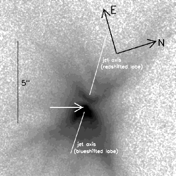
Figure 1: HST/WFPC2 image of LkH$\alpha$ 233 in the broad-band filter W814 (left panel). The axis of the bipolar jet (PA = 248^∘ for the blueshifted lobe) is indicated. The jet is not visible in this image because the signal is dominated by continuum emission from the reflection nebula surrounding the star. The maximum of the brightness distribution whose size scale is $0\aas@@fstack{\prime\prime}5\times 0\aas@@fstack{\prime\prime}5$ (marked with the white arrow in the left panel) is magnified in the right panel.

3 Results

3.1 The reflection nebula

The WFPC2 images in both broad-band filters clearly show a bipolar nebula with a dark lane between the two lobes (Fig. 1). This lane is already indicated by the Corcoran & Ray (1998) finding that the redshifted part of the bipolar jet is not visible for the first 0$\aas@@fstack{\prime\prime}$7 from its origin, which is probably due to circumstellar dust occulting the receding flow. Perrin et al. (2004) have observed the dark lane on a larger spatial scale (FWHM = 0$\aas@@fstack{\prime\prime}$27) using polarimetry in the near-infrared. The bipolar structure seen in Fig. 1 (left panel), together with the ‘spikes’ mentioned above, can thus be interpreted as a conical cavity cleared by the jet, as has also been suggested by Perrin et al. (2004). The optical emission comes from the inner edge of this cone that is illuminated by the star. An important consequence of this is that the optical and near-infrared brightness maximum does probably not coincide with the star itself, but with a region on the surface of the cone pointing towards us. This is supported by the finding that this maximum appears elongated and does not resemble a stellar PSF (Fig. 1, right panel). The interpretation of the brightness maximum as a scattering surface can also explain the extended structure found by Leinert et al. (1993) that was interpreted as a halo around the star in that work. From the present data, it is not clear if the ‘dark lane’ is a circumstellar disk seen close to edge-on or a dust torus around the star. If the former interpretation is true, LkH$\alpha$ 233 is one of the few young stellar objects where a disk has been directly observed. This disk, however, would have an apparent radius of about 1000 AU (adopting a size of the lane of approximately 1$\aas@@fstack{\prime\prime}$1 at a distance to LkH$\alpha$ 233 of 880 pc, see Fig. 1, left panel) and so it would be much larger than disks around classical T Tauri stars. The location of the bipolar jet is indicated in Fig. 1. It is, however, not visible there because the continuum emission from the reflection nebula overwhelms the line emission from the jet.

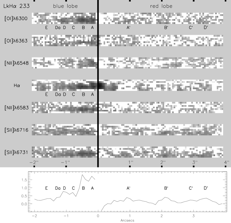
Figure 2: Images of the LkH$\alpha$ 233 jet in different emission lines, reconstructed from HST/STIS spectra, integrated over the full radial velocity range of the lines. The thick solid line marks the peak of the optical brightness distribution in the reflection nebula surrounding the star. The redshifted outflow lobe (PA = 68^∘) is on the right side of the image. Each panel has a spatial width of $\approx 0\aas@@fstack{\prime\prime}5$. The intensity is displayed logarithmically from $5\times 10^{-17}$ to $3\times 10^{-14}$ erg s^-1 cm^-2 arcsec^-2. For H$\alpha$ in the redshifted lobe, the signal is heavily affected by contributions from the disk/envelope in the first 0$\aas@@fstack{\prime\prime}$5 from the central position. The bottom panel shows the total flux distribution coadding all forbidden lines along the jet.

3.2 Jet structure

Spectroscopic data obtained with HST/STIS in the way described in Sect.  2, allow in principle to construct high angular resolution images of the flow in distinct velocity intervals. This is done by selecting the same velocity bin for each line in the S1…S7 spectra and aggregating the selected seven pixel columns in a 2D image. The result is analogous to what would be obtained with a high angular resolution integral field unit. This has been done successfully in the past for the jets from the classical T Tauri stars (CTTSs) DG Tau by Bacciotti et al. (2000) and RW Aur by Woitas et al. (2002). In the present case, however, the signal-to-noise ratio of the individual spectra of LkH$\alpha$ 233 is rather low. Therefore we could not reach a similar level of detail for this jet, but we aimed at constructing high angular resolution maps integrated spectrally, by coadding (after subtraction of the background) the column pixel values in each spectral channel. The resulting fluxes were strong enough to produce reconstructed images in each of the emission lines integrated over the whole radial velocity range covered by the lines with a sampling of 0$\aas@@fstack{\prime\prime}$05/pixel. Note that, since the STIS slit was moved from NW to SE, the numbering of the slit positions goes from S1 at the bottom pixel row of each panel to S7 at the top pixel row. The images in the emission lines included in the spectra are shown in Fig. 2. The lines are integrated over a velocity range of $\approx[0,225]\,\mathrm{km}\,\mathrm{s}^{-1}$ for the redshifted lobe and $\approx[0,-225]\,\mathrm{km}\,\mathrm{s}^{-1}$ for the blueshifted lobe, and the intensity varies logarithmically from $5\times 10^{-17}$ to $3\times 10^{-14}$ erg s^-1 cm^-2 arcsec^-2. To make positions of the jet knots more evident, we show in the bottom panel the total flux distrubution coadding all forbidden lines along the jet.

The redshifted lobe of the jet (PA = 68^∘), displayed in the right part of the image, is longer, but considerably fainter than the blueshifted outflow that occupies the lower part. The thick solid line marks the peak of the optical brightness distribution, which, as mentioned above, represents a bright point of the reflection nebula, and it is slightly displaced from the position of the star. This also caused the jet not to be centred on each individual panel, as explained above.

The blueshifted jet lobe is clearly visible in the STIS data within its first two arcseconds. Five jet knots (labelled A…E in Figs. 2 and 5) can be resolved in this region close to the star, with possibly an additional faint knot (that we labelled Da) between D and E. The knots are seen more clearly in [OI] $\lambda$6000, H$\alpha$, and [SII] $\lambda$6731, but they can also be distinguished in [NII] $\lambda$6583, where they appear to be more concentrated toward the jet axis. This is expected, since the [NII] lines are a tracer of higher excitation which, in turn, is expected to be found in the axial region, where the jet shocks are more powerful. If an arbitrary jet inclination of $45^{\circ}$ is assumed, the knot separations from the presumed position of the jet source are 200, 600, 1100, 1300, and 2100 AU, respectively. There is general consensus on the fact that bright knots trace the radiative cooling regions behind shock fronts, which form in the beam as a consequence of pulsation of the ejection mechanism at the jet base and/or internal instabilities during the propagation. The distance of the jet from Earth, however, does not allow the STIS resolution to ascertain whether the knots are actually bow-shaped, as seen in some other YSO jets. For the redshifted counter-jet, four jet knots (labelled $A^{\prime}...D^{\prime}$ in Fig. 2) are visible in the first $4^{\prime\prime}$ of the flow in [OI] $\lambda$6300 and [SII] $\lambda\lambda$6716,6731. The S/N ratio is, however, quite low here. We note that the knots in the two lobes are not placed symmetrically with respect to the source position, as one would expect if, e.g. the knots were due to instabilities in the accretion/ejection events. Similar asymmetries are found in many other bipolar jets, such as e.g., the flow from RW Aur (Woitas et al., 2002), but an explanation for these asymmetries is still lacking. Regarding the map in the H$\alpha$ line, we note that the emission of the jet was mixed with scattered light contributions from the disk and the envelope. We thus used the signal from $S6$ and $S7$, which contains no jet emission, to attempt a subtraction of these contributions. However, the result should be taken with care, especially within the first 0$\aas@@fstack{\prime\prime}$5 of the redshifted lobe. Here the signal appears to be heavily affected by the contributions from the disk/envelope and may not represent structures within the jet.

The same jet has been observed at much coarser spatial resolution by Corcoran & Ray (1998), who spectrally resolved several velocity components and determined corresponding electron densities, as shown in their Fig. 2. Taking the difference in spatial resolution into account, their results are in good agreement with our derivations. In Sect. 4 we will compare the images shown in Fig. 2 with analogous data resulting from high angular resolution analyses of the base of CTTS jets from other sources.

3.3 Physical quantities along the flow

Figure 3: Preliminary analysis of the ratios of selected forbidden lines along the blueshifted lobe of LkH$\alpha$ 233, integrated across the full velocity range and across the jet transverse section. Distances are from the brightness maximum of the circumstellar reflection nebula, here referred to as ‘source’. Top panel: [OI] $\lambda$6300/$\lambda$6363 with its error, compared with the theoretical ratio of Einstein’s A coefficients (dotted line). Bottom panel: same as above, for the [NII] $\lambda$6583/$\lambda$6548 ratio. In both panels discrepancies begin to be more evident from 1$\aas@@fstack{\prime\prime}$2 from the source.

Thanks to YSO jets possessing a rich spectrum of emission lines, one can determine many interesting physical quantities associated with the emitting gas. Besides the accurate measurements of the radial velocity through Doppler shifts, one can rely upon recently developed spectral diagnostic techniques to find, for example, the ionisation fraction, the total density, and the jet mass flux (Bacciotti & Eislöffel, 1999; Hartigan et al., 1994).

To find values of these quantities in the LkH$\alpha$ 233 jet, we follow a procedure described in Bacciotti & Eislöffel (1999), and subsequently refined and extended in Podio et al. (2006), usually referred to as the ‘BE technique’, which uses a combination of the forbidden lines from oxygen, sulphur, and nitrogen. These lines, excited collisionally, can be considered optically thin in the density and temperature regimes found in stellar jets and are easily modeled. The H$\alpha$ emission, albeit very strong, is not used in the diagnostics, because it is often contaminated by the reflection nebulosity around the star, it can suffer from absorption in high density zones, and it is produced by both collisional excitation and radiative recombination in regions not spatially coincident with the emission region of the forbidden lines (see Bacciotti & Eislöffel, 1999).

3.3.1 Preliminary analysis of the line ratios

Prior to the diagnostic analysis, the spectra were carefully examined, and it was found that the redshifted lobe of the jet is too faint in our images for the diagnostics to be applied at high angular resolution with a reasonable level of confidence. Thus for this lobe we integrated the signal spectrally and spatially in each of the four most prominent knots, and we applied the diagnostics to each knot as a whole (see Table 1).

For the brighter blueshifted lobe, the S/N was also not sufficient to perform a 2D diagnostic analysis. Therefore, we integrated spectrally and across the jet, and the high angular resolution information was only retained for the direction along the flow. For the blue-shifted lobe, we then formed various ratios of the forbidden lines to check for the presence of evident problems of S/N, that may render these lines unusable in certain locations. The ratios [OI] $\lambda$6300/$\lambda$6363 and [NII] $\lambda$6583/$\lambda$6548 should equal the ratio of Einstein’s A coefficients for spontaneous emission, which is about 3 in both cases. Departure from this value can give an idea of the regions of the jet where the diagnostics will be less reliable due to poor S/N. The comparison is shown in Fig. 3 with the theoretical value, and the line fluxes were integrated across the jet and in radial velocity, with errors propagated quadratically.

The comparison shows that the observed points are fairly close to the theoretical line until about $1\aas@@fstack{\prime\prime}2$ from the source, corresponding to the tip of knot D in Fig 2. Beyond 1$\aas@@fstack{\prime\prime}$2 and up to 1$\aas@@fstack{\prime\prime}$7, corresponding to a faint region of the jet, the observed ratio deviates from the expected value. The ratio of oxygen lines is acceptable again at the end of the jet at the location of knot E, while for nitrogen lines the ratio is still far from the expected one at this position. Our test implies that the diagnostic results for the regions of the flow farther from the source than knot D should be taken with caution, especially for the ionisation fraction, which is tightly correlated with the [NII] measurements. Since it is likely that these problems are caused by the very low S/N of the faintest lines in each of these pairs, we decided to use the flux of the brightest one and the theoretical ratio for our subsequent excitation analysis.

The top panel of Fig. 4 illustrates the values of the ratio [SII]$\lambda$6716/$\lambda$6731. From this ratio one can measure the electron density along the flow. The theoretical value of the ratio calculated for $T_{\mathrm{e}}=10^{4}$ K in both the low and high density limits are superimposed on the datapoints. The critical density for this ratio (corresponding to the high density limit) is $2.5\times 10^{4}$ cm^-3, while $n_{\mathrm{e}}$ = 50 cm^-3 is the minimum value for the subsequent diagnostics to be applicable. From the plot, one can argue that the electron density along this jet is very high along the first 1″ from the source, while it clearly drops at greater distances, despite the larger measurement errors. Where the measured [SII] $\lambda$6716/$\lambda$6731 values are outside the indicated range (because of poor S/N), the data can only provide upper/lower limits to the electron density, indicated in the following plots with arrows.

Figure 4: Preliminary analysis of the line ratios used for the diagnostics along the blueshifted lobe of LkH$\alpha$ 233. Fluxes are integrated across velocity and spatially across the jet transverse section. Distances are from the brightness maximum of the circumstellar reflection nebula. Top panel: [SII] $\lambda$6716/$\lambda$6731 ratio with its measurement error. The theoretical value in the low density limit (dotted line) and high density limit (dot-dashed line), calculated for $T_{\mathrm{e}}=10^{4}$ K are superimposed. Middle panel: ratio [NII] $\lambda$(6548+6583)/[OI] $\lambda$(6300+6363), with its error. This ratio is very sensitive to the hydrogen ionisation fraction (see text). Bottom panel: variation of the ratio [OI] $\lambda$(6300+6363)/[SII] $\lambda$(6716+6731), which is sensitive to both the electron temperature and the ionisation fraction of the emitting gas.

In Fig. 4, we also report the observed value of the ratios [NII] $\lambda$(6548+6583)/[OI] $\lambda$(6300+6363) (hereafter referred to as [NII]/[OI], middle panel) and [OI] $\lambda$(6300+6363)/[SII] $\lambda$(6716+6731) (hereafter [OI]/[SII], bottom panel), integrated in velocity and across the jet cross section, with errors propagated quadratically. As shown in Bacciotti & Eislöffel (1999), the [NII]/[OI] ratio only depends weakly on temperature, but it is a good indicator of the level of global ionisation in the flow, since the ionisation fractions of N and O are tightly correlated to that of hydrogen through charge exchange reactions. The plot shows a gradual increase in this ratio, and hence of ionisation, going from the source to the position of knot C. Then the values decline to a minimum in the region of faint flux around 1$\aas@@fstack{\prime\prime}$4 from the source. The ratio then appears to increase substantially at the end of the flow; however, this may not be real due to the aforementioned measurement problems for the [NII] line fluxes. The [OI]/[SII] ratio depends on both the hydrogen ionisation fraction and the electron temperature in the gas, but is correlated more tightly with the latter. The values of the ratio first decrease from the source to a minimum at 0$\aas@@fstack{\prime\prime}$2, followed by a gradual increase along the jet, with the highest values reached at the position of knot C, and a minimum immediately downstream of knot D. The values of this ratio, however, are defined better toward the end of the flow with respect to the [NII]/[OI] ratio.

3.3.2 Results of spectral diagnostics

In this paragraph we present the results of the BE diagnostic procedure described in Bacciotti & Eislöffel (1999) applied to our dataset. Basically, the various quantities are obtained by comparing the observed line ratios with those calculated by a code designed to predict the fluxes in forbidden lines starting from a grid of values of electron density $n_{\mathrm{e}}$, hydrogen ionisation fraction $x_{\mathrm{e}}$, and electron temperature $T_{\mathrm{e}}$. The electron density is obtained by inverting the ratio of sulphur lines, which is independent of $x_{\mathrm{e}}$ and only weakly dependent on $T_{\mathrm{e}}$. Then, $x_{\mathrm{e}}$ and $T_{\mathrm{e}}$ are found by combining and inverting the [OI]/[NII] and [OI]/[SII] ratios, also using the retrieved $n_{\mathrm{e}}$. The calculation was performed with a numerical code developed by one of us (U. Locatelli) to apply the technique to large datasets. For more details on the diagnostic technique and on the underlying physical assumptions, together with its limits of application, see Bacciotti (2002) and Podio et al. (2006).

Due to the aforementioned problems of poor S/N, we performed the diagnostic analysis on the ratios obtained integrating the spectral datacube both in velocity and in the spatial direction across the jet. Thus high angular resolution is retained only for the direction along the flow. We stress that, in the present case, due to the problems of low S/N, we only use the brightest lines of the [OI] and [NII] doublets to form the observed ratios that will be compared with the theoretical ones in the diagnostics (see Sect. 3.3.1).

The results of the diagnostics are collected in Fig. 5. The figure, in the first two panels, also illustrates the intensity profile of the emission lines and the radial velocity of the material at each position along the jet, to give a positional and kinematical reference for the values of the thermal properties shown in the other panels.

The line flux distribution along the flow (top panel) is derived from the sum of the spectroscopic images in [OI] $\lambda\lambda$6000,6363, [NII] $\lambda\lambda$6548,6583, and [SII] $\lambda\lambda$6716,6731, and subsequent integration of the combined image across the jet axis. As mentioned above, this step was necessary to reach a sufficient S/N ratio for application of the diagnostics.

The information about the jet structure is complemented by determining of the radial velocity of each feature in the [SII] $\lambda$6731 and the [OI] $\lambda$6300 lines (second panel from top). This was obtained by summing the spectra in the direction transverse to the jet, which is coadding the individual $S1$…$S7$ and then performing Gaussian fits to the integrated (spatially) line profile in each pixel row. This yielded peak radial velocities versus distance from the source, which were then transformed to systemic velocities assuming the heliocentric radial velocity of LkH$\alpha$ 233 to be $-17.2\,\mathrm{km}\,\mathrm{s}^{-1}$ (see Sect. 1).

The velocities along the line of sight vary between $-60$ km s^-1 close to the star and $-160$ km s^-1 at the end of the observed portion of the jet. Errors are not reported on each point to keep the plot readable, but these were accurately determined from the Gaussian fit and vary between 10 and 40 km s^-1 for both lines, being greater toward the end of the flow, which is fainter. For the redshifted lobe, no precise Gaussian fit was possible due to the low S/N. A rough estimate of the line shifts, however, indicated velocities of the plasma of about the same amplitude as in the blue lobe.

The velocity determinations indicate a gradual increase in velocity with distance in the examined jet portion. This increase is, however, not continuous, as the velocity is fairly constant along the first 0$\aas@@fstack{\prime\prime}$9 of the jet (the brightest jet portion), and then presents sudden jumps at knots D and E. This probably indicates that the last two knots move into a more rarefied external medium. Internally to almost all of the knots, one can marginally distinguish a local decrease in the radial velocity across each knot, revealed in both lines. For an interpretation of this effect, see Sect. 4.

Figure 5: Physical properties of the emitting gas in the blueshifted lobe of the bipolar jet from LkH$\alpha$ 233 as a function of distance from the brightness maximum of the circumstellar reflection nebula. All quantities (except the radial velocity) are derived after integration across wavelength and across the jet width. From top to bottom: intensity profile resulting from the sum of forbidden line fluxes, in units of $10^{-14}$ erg s^-1 cm^-2 arcsec^-1 (letters refer to the jet knots displayed in Fig.2); radial velocity resulting from the analysis of the lines [OI] $\lambda$6300 and [SII] $\lambda$6731, integrated across the jet (errors range between 10 and 40 km s^-1, see text); electron density $n_{\mathrm{e}}$; hydrogen ionisation fraction $x_{\mathrm{e}}$; electron temperature $T_{\mathrm{e}}$; total density $n_{\mathrm{H}}=n_{\mathrm{e}}/x_{\mathrm{e}}$; mass loss rate $\dot{M}_{\mathrm{J}}$.

The lower panels of Fig. 5 illustrate the thermal properties in the blueshifted lobe of the jet, resulting from the application of the BE technique.

The third panel from top describes the variation in the electron density, $n_{\mathrm{e}}$, along the jet, as derived from the inversion of the ratio of the two sulphur lines for an assumed temperature of 10⁴ K. The reported errors on $n_{\mathrm{e}}$ come mainly from the propagation of the S/N uncertainty of the [SII] lines, with a smaller contribution from the a priori uncertainty of $T_{\mathrm{e}}$, although the line ratio is only weakly sensitive to this parameter. ‘Upward’ arrows are lower limits, equal to the critical density, in the positions where the ratio reached its saturation value. Similarly, ‘downward’ arrows indicate positions where the electron density is lower than 50 cm^-3 (the limit of applicability of the BE technique). As already argued from the inspection of Fig. 4, the electron density is quite high in the first portion of the flow. Its value scatters around 10⁴ cm^-3 in the first 0$\aas@@fstack{\prime\prime}$5 and then gently decreases down to 10³ cm^-3 at 0$\aas@@fstack{\prime\prime}$75, corresponding to the base of knot C. It is then apparently extremely high inside this knot, even though the corresponding line brightness is not exceedingly large. The region downstream of knot C presents a different character; since it is much less dense in free electrons. Here $n_{\mathrm{e}}$ scatters between 500 to 1000 cm^-3, apart from those positions where the lower limit is reached, and an isolated point of higher density in knot E. Overall, the situation appears to be consistent with the jet experiencing less confinement by the surrounding medium downstream of knot C.

In the fourth and fifth panels from top, we illustrate the results of the BE diagnostics for the hydrogen ionisation fraction $x_{\mathrm{e}}$ and the electron temperature $T_{\mathrm{e}}$ along the blueshifted jet. In determining these quantities, great attention has been devoted to a realistic estimate of the errors, as there are a number of different sources of uncertainty in this case. First of all, the diagnostic uses ratios of lines produced by different elements, therefore an assumption of the set of elemental abundances is necessary. This aspect is extensively analysed in Podio et al. (2006), where the authors conclude that solar abundances are not adequate in all cases, but instead the abundance set appropriate for the region under study should be chosen. Unfortunately, no determination of abundances exists in the literature for the Lacerta Cloud, so we have adopted the abundance set of Orion by Esteban et al. (2004), assuming that the two regions have been exposed to the same enrichment processes (see Neufeld et al., 2006). Another source of error comes from the uncertainty in $n_{\mathrm{e}}$, which is an input of the diagnostic calculation. We then have to consider the measurement error of the ratios [NII]/[OI] and [SII]/[OI], as displayed in Fig. 4, which includes both the S/N accuracy and the effect of variations in extinction along the jet beam that are unaccounted for.

All these sources of error were considered and their effect on the final determination of $x_{\mathrm{e}}$ and $T_{\mathrm{e}}$ was found a posteriori by running the code at the extremes of the range of variations in the input quantities. The resulting uncertainties are displayed as error bars in the panels. These are limited to 15–20% in the bright part of the jet, but they rise up to 50–60% on average in the faint final section. Missing points are due to the fact that in those positions the values of the ratios fall out of the range of validity of the technique. This basically occurs in regions of poor S/N in the [NII] lines, but see Podio et al. (2006) for a more detailed discussion of this point. It has also to be kept in mind that the positions where the electron density was only determined as a lower limit are critical, and the results for $x_{\mathrm{e}}$ and $T_{\mathrm{e}}$ must be taken with caution in these regions. A better determination of the electron density in these positions would be desirable, but this would require the use of pairs of lines of higher critical density not included in our STIS setting. To overcome this problem, Hartigan & Morse (2007) have recently attempted a simultaneous inversion of all the line ratios available from similar STIS spectra of HH 30 in the high density regions toward the star. The results for HH 30 are encouraging, but the mathematical complexity involved in implementing our code along the same lines does not seem justified by the very limited number of positions in this jet where the [SII] ratio gives poor information.

Despite the many sources of error discussed above, our diagnostics allowed us to establish with reasonable accuracy both the value and the variation in the ionisation fraction and the electron temperature in most of locations along the jet. In the first bright portion $x_{\mathrm{e}}$ appears on average to increase from about 0.2 in knot A up to 0.6 in knot C, where the jet shows the maximum ionisation. Note that the latter corresponds to a lower limit determination of the density, which may lead to a possible overestimate of the ionisation fraction. An inspection of Fig. 4, however, reveals that the [NII]/[OI] ratio itself presents a peak in that position, which lead us to believe that the enhancement of ionisation in this knot is real. Downstream of knot C $x_{\mathrm{e}}$ falls again to values around 0.3, but it clearly rises again in knot E up to $0.4-0.5$. While the variations are moderate, they are nevertheless evident, and we note no clear association between peak intensity and peak ionisation inside each knot.

The electron temperature $T_{\mathrm{e}}$ in the jet ranges between 1 and $3\times 10^{4}$ K, and its pattern of variation is complex, too. The value of $T_{\mathrm{e}}$ shows a marked decrease in the first $0\aas@@fstack{\prime\prime}3$ inside knot A, down to 10⁴ K at 0$\aas@@fstack{\prime\prime}$25, and it then turns up again to $3\times 10^{4}$ K at the end of knot B. The temperature shows a minimum in knot C, but here again the decrease to $7000-8000$ K may be artificially caused by the poor determination of the electron density in this knot. In knot D there are less positions in which the diagnostic is applicable. Here, $T_{\mathrm{e}}$ first appears to increase again to $3-4\times 10^{4}$ K at 1$\aas@@fstack{\prime\prime}$1 from the source and then to decrease to $1.5-2\times 10^{4}$ K in knots Da and in the first part of knot E. There is a final local peak of the temperature to $2.2\times 10^{4}$ K toward the second half of knot E.

Once $x_{\mathrm{e}}$ and $n_{\mathrm{e}}$ are determined, a rough estimate of the average total hydrogen density $n_{\mathrm{H}}$ can then be derived as $n_{\mathrm{H}}=n_{\mathrm{e}}/x_{\mathrm{e}}$ (errors are propagated quadratically from these quantities). Note, however, that this simple calculation likely overestimates the actual average densities in the jet by a factor $3-5$, because the determination is biased toward the regions of higher line brightness, which in turn are those of higher compression after a shock front. Nevertheless, it is extremely useful to have at least an approximate value for this parameter, because the total density enters all the relationships governing the dynamics of the jet. In particular, it is extremely important to know this parameter when attempting a comparison between the analytical and numerical model predictions and the actual observations. The jet appears to be quite dense in the initial portion, as the hydrogen total density varies between 10⁴ and 10⁵ cm^-3 in knots A–D. Of course, the lower limits found for $n_{\mathrm{e}}$ affect density estimations inside knot C. Downstream of knot D, $n_{\mathrm{H}}$ presents lower values, scattering on average around $5\times 10^{4}$ cm^-3. Overall, the jet from this source appears to be one of the densest studied so far with the BE diagnostics.

Table 1: Physical quantities in the redshifted lobe of the jet from LkH$\alpha$ 233, averaged spatially and spectrally over each jet knots (see text).

Knot	Location	$\log(n_{\mathrm{e}})$	$x_{\mathrm{e}}$	$\log(n_{\mathrm{H}})$	$\dot{M}_{\mathrm{J}}$
	(′′)	(cm-3)		(cm-3)	(10-7 M☉ yr-1)
$A^{\prime}$	$0.65-1.00$	4.06	0.12	4.98	3.7
$B^{\prime}$	$1.85-2.50$	3.85	0.19	4.58	1.5
$C^{\prime}$	$2.55-2.95$	3.94	0.47	4.26	0.7
$D^{\prime}$	$3.00-3.45$	3.90	0.20	4.59	1.5

The last panel of Fig. 5 illustrates our estimate of the mass flux in the jet. This is discussed in detail in the next section.

We conclude this part by commenting briefly on the diagnostic results obtained for the red lobe, from the data integrated spectrally and spatially in each knot (see Table 1). The excitation conditions are quite different here from those found in the blue lobe, which is already indicated by the fact that this counter-jet is more prominent in [SII] $\lambda\lambda 6716,6731$ than in [OI] $\lambda 6300$, in contrast to the blueshifted lobe. From the table one can see that $n_{\mathrm{e}}$, $x_{\mathrm{e}}$, and $n_{\mathrm{H}}$ are all lower in the redshifted lobe than in the blueshifted one. In particular $n_{\mathrm{e}}<n_{\mathrm{crit}}$ of the sulphur lines for all the knots investigated here. The maximum electron density is found in knot A^′, where it is about 10⁴ cm^-3. It then decreases in the other knots, but it is never less than 8000 cm^-3. On the other hand, the ionisation fraction is generally not more than $10-20$%, if exception is made for knot C^′, which seems quite excited, reaching $x_{\mathrm{e}}\sim 0.5$. The combination of $x_{\mathrm{e}}$ and $n_{\mathrm{e}}$ provides quite a high total density that decreases from 10⁵ cm^-3 at the base of the jet down to $\sim 1.8\times 10^{4}$ cm^-3 in knot C^′. The electron temperature is around $1-2\times 10^{4}$ K. Because of the low signal in [OI] lines, however, the estimate is not as detailed as in the blue lobe, so values are not given in the table. We instead attempted an estimate of the mass flux, which is discussed in the following section.

4 Discussion

4.1 Mass flux in the jet

One of the most useful quantities to know when comparing models with observations in the case of jets is the mass flux in the outflow, $\dot{M}_{\mathrm{J}}$, and its variation along the flow. For example, in the magnetohydrodynamic (MHD) models proposed to explain the formation of YSOs, the ratio between ejected and accreted matter around the star is fixed ($\dot{M}_{\mathrm{J}}/\dot{M}_{\rm acc}\sim 0.01\div 0.1$). Moreover the knowledge of $\dot{M}_{\mathrm{J}}$ allows us to estimate other important dynamical quantities like the linear and angular momentum carried by the jet (adding the information on poloidal and, where available, toroidal velocities). In turn, these estimates can clarify if the jet is capable of accelerating coaxial outflows, to clear the stellar environment and to inject turbulence in the cloud (Podio et al., 2006), as well as to extract the excess angular momentum from the disk/star system (see e.g. Woitas et al., 2005).

In principle we can determine the mass flux from the emission lines in two ways, described in detail in Nisini et al. (2005). In the first method, the mass flux at each position is estimated by combining the total density inferred from diagnostic techniques with the values of the jet radius and velocities, $r_{\mathrm{J}}$ and $v_{\mathrm{J}}$, provided by the FWHM of the luminosity profile across the jet and the kinematical analysis, respectively. This approach assumes that each considered ‘slice’ of the jet is uniformly filled at the density derived from the diagnostics, which is biased toward more compressed regions. The second method compares the observed luminosities of the forbidden lines to the one calculated by an emission model, thus providing the mass of the emitting gas. This method implicitly takes the filling factor into account, but is affected by uncertainties in absolute calibrations, extinction, abundance, and distance. In our case, the problems of an unknown filling factor is mitigated by our observing the jet close to the source and at high angular resolution, which limits the possibility of including large regions of non-emitting material in the beam. On the other hand, extinction, elemental abundances, and distance are not well known in our case. Therefore, we prefer to use the first method, keeping in mind that the derived values of $\dot{M}_{\mathrm{J}}$ have to be considered as upper limits. Previous studies performed on other jets by applying both methods show that the mass flux derived in this way is overestimated by not more than 20% when high angular resolution is used (Bacciotti et al., 1999).

With our estimate of $n_{\mathrm{H}}$, the mass flux can be computed as $\dot{M}_{\mathrm{J}}=\mu m_{p}n_{\mathrm{H}}\,\pi\,r_{\mathrm{J}}^{2}\,v_{\mathrm{J}},$ where $r_{\mathrm{J}}$ is the jet radius, $v_{\mathrm{J}}$ the full spatial velocity, $m_{p}$ the proton mass, and $\mu$ the mean molecular weight, equal to $\sim$ 1.24 for interstellar atomic gas in standard composition. In our case, the jet radius was estimated taking half the FWHM obtained from Gaussian fits to the sum of all spectroscopic maps in forbidden emission lines, which is nearly constant at $\approx 100$ AU between $d=0\aas@@fstack{\prime\prime}1$ and 0$\aas@@fstack{\prime\prime}$6. As the S/N is not high enough to derive reliable results beyond $d=$ 0$\aas@@fstack{\prime\prime}$6, we assume the jet radius to be the same there as closer to the origin, i. e. $r_{\mathrm{J}}=50\,\mathrm{AU}$. The flow velocity $v_{\mathrm{J}}$ is derived from fits to the coadded spectra $S1...S7$ in [OI] $\lambda$6300 and [SII] $\lambda$6731, as mentioned above, and de-projected with an arbitrary inclination angle of $i=45^{\circ}$. The resulting mass flux in each position of the blueshifted lobe is shown in the bottom panel of Fig. 5 (errors also include the uncertainties on $v_{\mathrm{J}}$ and $r_{\mathrm{J}}$ estimated from the Gaussian fit to the profiles of the emission lines). The mass flux appears to be fairly constant at a value of about $10^{-7}$ M_☉ yr^-1 between the source and knot C, indicating that the flow is well-collimated in this portion and that turbulent interaction with the external medium, which may change the amount of transported mass, is negligible. The mass flux then decreases by $1-2$ orders of magnitude in the last part of the jet. This could be because the real jet radius is actually larger than the one assumed. The fact that the jet undergoes lateral expansion downstream of knot C is also supported by the marked change of the other physical properties derived by the diagnostics. Alternatively, a significant portion of the mass could have been ejected sideways by the bow shocks in the working surfaces during the jet propagation, or $\dot{M}_{\mathrm{J}}$ may be higher now than it was in the past.

Regarding the redshifted lobe, for which our derivations come from data integrated spatially and spectrally on each condensation, we can estimate the mass flux averaged over each knot as was done, e.g., in Podio et al. (2006). To this purpose, we assume a de-projected flow velocity of 170 km s^-1 and a jet diameter of 100 AU, similar to the blueshifted lobe. The obtained values are reported in Table 1. The resulting mass flux in the counter-jet seems to have the same order as in the blueshifted jet, with a maximum for knot $A^{\prime}$, where we obtain $\dot{M}_{\mathrm{J}}\sim 3.7\times 10^{-7}M_{\sun}$ yr^-1, and lower values in the following knots, but still the same order of magnitude.

Overall, the value of the observed mass flux in proximity to the star is slightly above the upper boundary of the values obtained for the jets from T Tauri stars. If the ratio of accreted-to-ejected mass flux is regulated as suggested by standard MHD jet launching models, the results would imply a mass accretion, $\dot{M}_{\rm acc}$, onto the star of the order of several $10^{-6}M_{\sun}$ yr^-1.

4.2 Nature of the knots

In the second panel of Fig. 5, internal to almost all of the knots, one can marginally distinguish a local decrease in the velocity, revealed in both the [OI] and [SII] lines. This is consistent with the knots being mini-working surfaces, which should form inside the jet according to some models of jet propagation, and are also directly imaged in resolution observations of T Tauri jets (Ray et al., 1996). Each working surface is contained within two shocks, one on the side of the jet source, the so-called Mach disk, in which the high velocity material of the jet beam coming from the source is decelerated upon entering the working surface. The other shock is on the downstream side, the bow-shock, in which the material ahead and moving more slowly than the shock front, is accelerated upon entering the working surface. The cooling region of the working surface is located between the two shocks and can be assumed to extend about 10¹⁵ cm, which is the same scale as the knots observed in this flow. It is therefore reasonable to interpret the local variation in the velocity observed within each knot as a consequence of the combined action of the two shocks constituting a working surface. In this framework, the slight differences in the position of the velocity variations in the two emission lines can be due to the peak emission region of the two species behind a shock front being slightly displaced (Bacciotti & Eislöffel, 1999). In conclusion, even if a bow-shaped morphology of the knots is not directly identified in the image of this flow, the velocity pattern appears to point toward a similarity of the knot properties with those of the TTS jets.

4.3 Comparison with flows from lower mass stars

These findings can be compared with studies of other jets from T Tauri stars studied at high angular resolution and/or analysed with the same diagnostic method. The HH~30, DG Tau, and RW Aur jets were observed at high angular resolution with HST close to their sources ($d\leq 1000\,\mathrm{AU}$) (Ray et al., 1996; Bacciotti et al., 1999, 2000; Bacciotti, 2002; Woitas et al., 2002; Hartigan & Morse, 2007) and from the ground with the CFHT using adaptive optics techniques (Dougados et al., 2000). These jets were then analysed with the same diagnostic technique used here. Several other jets (HH~34, HH~1, HH~111, HH~46/47, HH~24, HH~83, HH~30, HL~Tau, and Th~15-28) were observed from the ground on much larger spatial scales of 1000 to some 10000 AU from their parent stars and analysed with the BE technique (Bacciotti & Eislöffel, 1999; Nisini et al., 2005; Podio et al., 2006). In these cases the sources are either deeply embedded protostars or T Tauri stars.

In the first $\approx 2000$ AU of the blueshifted LkH$\alpha$ 233 jet, the electron density $n_{\mathrm{e}}$ is remarkably higher than the one found in jets at large distance from the star, but similar to the electron density values found at the base of the jets observed at high angular resolution (Bacciotti et al., 2000; Bacciotti, 2002). On larger scales $n_{\mathrm{e}}$ is expected to decrease due to recombination and the widening of the flow.

In the HH 30 jet, analysed at high spatial resolution, the ionisation is lower on the whole than in LkH$\alpha$ 233. Likewise, it is rising in the first part of the flow and reaches its first maximum at $d\approx 300$ AU (in contrast to $d\approx 500$ AU for LkH$\alpha$ 233). In the same region the temperature decreases steeply from $2\times 10^{4}$ to less than $10^{4}$ K. Similar behaviour is also seen in the DG Tau and RW Aur jets observed with HST at high angular resolution (Bacciotti 2002, Bacciotti et al. in preparation, Melnikov et al. in preparation), thus this appears to be a common phenomenon. Several studies have indeed recently tried to justify these trends in the framework of jet acceleration models (cf. Shang et al., 2002; Garcia et al., 2001). Alternatively, knot A might trace the presence of a strong shock, where $T_{\mathrm{e}}$ is high and $x_{\mathrm{e}}$ first increases to reach a plateau and then ‘freezes’ and slowly recombines along the flow (cf. Bacciotti & Eislöffel, 1999). For the other jets studied on larger angular scales, the ionisation is of the same order of magnitude as for LkH$\alpha$ 233. Re-ionisation events are found in a number of these outflows, but they occur on a much larger spatial scale than in the jet studied here.

The total density in the LkH$\alpha$ 233 jet, derived by combining the ionisation fraction and electron density, is quite high, at least in its initial part, reaching 10⁵ cm^-3. Overall, the jet from this source appears to be the densest studied so far with the BE diagnostics.

The electron temperature $T_{\mathrm{e}}$ in the LkH$\alpha$ 233 jet is of the same order of magnitude as for the other jets. Peaks of $T_{\mathrm{e}}$ along the jet, as in the blueshifted lobe of the LkH$\alpha$ 233 jet, can also be seen in the outflows of HH 46/47, HH 24 C, and HL Tau, but again at much larger separations from their respective sources. Finally, the observed flow velocity is not very different from that of T Tauri jets.

The mass loss rate is another fundamental parameter for testing the similarity of the physics in YSO outflows. In the case of LkH$\alpha$ 233 the mass loss rate is in general larger by up to one order of magnitude than for the jets observed on extended scales. It is, however, only slightly higher than the values found for other jets from lower mass stars studied at high angular resolution close to the source. In conclusion, the physical properties of this jet appear similar to those of classical T Tauri stars, apart from an enhancement of the total density.

Garcia Lopez et al. (2006) have determined accretion rates for a number of Herbig stars using a well-established correlation between $L($Br${}_{\gamma})$ and the accretion luminosity $L_{\mathrm{acc}}$. For a set of 36 Herbig stars, they found that 80% are accreting matter at rates of $3\times 10^{-9}\lesssim\dot{M}_{\mathrm{acc}}\lesssim 10^{-6}M_{\sun}$ yr^-1. If we adopt a mass flux for LkH$\alpha$ 233 of about 10% of its mass accretion rate (according to MHD models), then the $\dot{M}_{\mathrm{acc}}\sim 10^{-6}M_{\sun}$ yr^-1 (taking a smaller fraction of ejected to accreted matter would lead to an even higher value of $\dot{M}_{\mathrm{acc}}$). This would make LkH$\alpha$ 233 one of the strongest accretors among the Herbig stars. Garcia Lopez et al. (2006) also found that the $\dot{M}_{\mathrm{acc}}$ distribution of Herbig stars is roughly consistent with the prediction of a $\dot{M}_{\mathrm{acc}}\propto M_{\star}^{1.8}$ relation derived for subsolar mass objects and noticed a deficit of very strong accretors with rates higher than $10^{-7}M_{\sun}$ yr^-1. They suggested that this deficit could be due to an “aging”-effect, since the accretion rate is expected to decrease with time (Hartmann et al., 1998). From this point of view LkH$\alpha$ 233 would be a very young Herbig star with a very high accretion rate in which the jet carries away an excess of angular momentum.

5 Conclusions

We have analysed images and spectra of the immediate environment of the Herbig Ae/Be star LkH$\alpha$ 233 taken in the visible range with the Hubble Space Telescope, which provides unprecedented high spatial resolution (0$\aas@@fstack{\prime\prime}$1 in the optical). The observed brightness distribution in archival HST images is probably from the surface of a cone; i. e. we do not see the source directly. We infer that a disk or dusty torus obscures the star. The brightness of the nebula does not allow one to see the jet in filtered narrowband ($\Delta\lambda\approx 50$ Å) images, but it could be imaged in 2D maps derived from STIS data, reconstructing images of the flow in the various lines integrated in velocity from a set of seven spectra taken by stepping the slit in adjacent positions.

In this way, we have resolved fine structure in the distant bipolar jet from LkH$\alpha$ 233 (880 pc), in both the blueshifted and redshifted lobes. Within its first arcseconds ($\approx 2000$ AU), the jet knots appear circular or elliptical at HST resolution, although the kinematical analysis reveals that they probably trace mini-working surfaces, as is common in stellar jets.

We have analysed the spectroscopic maps with a diagnostic code designed to adapt the so-called BE technique (Bacciotti & Eislöffel, 1999) to large datasets. The low values of S/N of the spectra forced us to integrate the maps across the jet width in the blue-shifted lobe, and across the extension of each knot in the red lobe, in order to have acceptable inputs for the diagnostic technique. The results are displayed in Fig. 5 and Table 1, respectively. High angular resolution is retained along the jet axis in the blueshifted lobe.

The electron density in the first arcsecond of the blueshifted lobe is about 10⁴ cm^-3, close to the critical density for [SII] emission and, in a few positions, is above the critical value. The electron density decreases along the flow by slightly more than one order of magnitude, reaching values of about $800-1000$ cm^-3 at the position of the last visible knot (2^′′ from the source).

The hydrogen ionisation fraction in the same lobe varies between 0.2 and 0.6. It gently rises on the first 500 AU of the flow, like other jets from young stellar objects studied at high angular resolution; but instead of reaching a plateau followed by slow decay, it goes through apparent episodes of re-ionisation along the flow.

The electron temperature $T_{\mathrm{e}}$ found with the diagnostics varies between 1 and $3\times 10^{4}$ K, in agreement with the kind of lines observed. The jet knot A, located closest to the origin, is correlated with a maximum of the electron temperature and might represent a strong shock. In the region of jet knot C, there appears to be an anti-correlation between $T_{\mathrm{e}}$ and ionisation. The nature of this anti-correlation is unclear, but the result for the temperature here might have been affected by quenching of the [SII] lines.

Combining the values of $x_{\mathrm{e}}$ and $n_{\mathrm{e}}$ we obtained estimates of the total density in this flow. The jet appears to be quite dense, especially close to the star; and with its $n_{\mathrm{H}}\sim 10^{5}$ cm^-3, it turns out to be the densest outflow studied with the BE technique so far.

The mass flux $\dot{M_{\mathrm{J}}}$ is $\approx 10^{-7}$ M_☉ yr^-1 in the first arcsecond of the jet, while it decays by an order of magnitude further out. These values are slightly higher than the mass-loss rate measured for the jets from lower mass YSOs. This is the first determination of a mass flux rate of a jet from a Herbig star obtained with the same method as for T Tauri jets.

In the redshifted counter-jet, electron density, ionisation, and mass density are all lower than in the blueshifted jet and are consistent with a lower degree of excitation.

We have compared the outcomes of our study with the properties of jets from T Tauri stars studied previously with the same diagnostics. The physical properties of the jet from this HAeBe star appear totally analogous to those in T Tauri jets, scaled toward higher densities and higher mass-loss rates. This appears to be consistent with a similar accretion/ejection engine in the two classes, with an enhanced rate of mass accretion onto HAeBes with respect to TTSs.

Overall, these results suggest the same type of ‘engine’ drives the accretion/ejection in intermediate and low mass stars as well as sub-stellar objects.