Conductance Through Graphene Bends and Polygons

Abstract

We investigate the transmission of electrons between conducting nanoribbon leads oriented at multiples of 60^∘ with respect to one another, connected either directly or through graphene polygons. A mode-matching analysis suggests that the transmission at low-energies is sensitive to the precise way in which the ribbons are joined. Most strikingly, we find that armchair leads forming 120^∘ angles can support either a large transmission or a highly suppressed transmission, depending on the specific geometry. Tight-binding calculations demonstrate the effects in detail, and are also used to study transmission at higher energies as well as for zigzag ribbon leads.

I Introduction

Graphene, a two-dimensional honeycomb lattice of carbon, is one of the most interesting new low-dimensional materials to have become available in the laboratory in the last few years novoselov . When undoped, the low energy physics of this system is dominated by two Dirac points review . The wavefunctions associated with states near them are described by spinors, whose amplitudes represent the probability density to find electrons on either of the two honeycomb sublattices. Because the fermion spectrum is gapless, these spinors have well-defined helicity, leading to an absence of backscattering from impurities review2 ; shon . The observed metallic behavior of undoped graphene is likely to be a manifestation of this suppressed backscattering novoselov .

Among the interesting and potentially useful properties of graphene is the prospect of “tailoring” its electronic properties by cutting it into ribbons of well-defined widths along various symmetry directions review ; brey1 ; brey2 ; brey3 . Recent experimental work han ; chen ; li has confirmed the possibility of tuning transport gaps of graphene ribbons via their widths, although the quality of these ribbons is not yet high enough to be usefully compared with the expected brey1 width dependence of ideal ribbons. In applications one generically needs to join such ribbons together as interconnecting wires or elements of a device. Understanding the transport through such junctions is then important in designing graphene geometries with desirable behaviors. This the subject of our study.

Changing the direction of electron currents would presumably be an important aspect of any graphene-based circuit. In both quantum wires and electromagnetic waveguides it is known londergan that the transmission through bends depends on the detailed nature of the bend geometry. This raises the prospect that the conductive behavior of a graphene junction may differ substantially from the properties of its individual nanoribbon leads.

In the simplest situation, the nanoribbon leads meeting at a junction are of the same type (armchair or zigzag), restricting the bend angles to either 60^∘ or 120^∘. The latter case is particularly interesting due to the behavior of the low energy states near the Dirac points under 60^∘ rotation. These states may be constructed, within the ${\bf k}\cdot{\bf p}$ approximation, from products of the exact wavefunctions at the Dirac points, which vary rapidly in real space, with slowly varying envelope functions review2 . The rotation induces a transformation on the fast component of the wavefunction which exchanges both the valleys and the sublattices. As a result, states near the Dirac points are nearly orthogonal to their 60 degree rotation in a confined geometry. Since a ribbon with a 120^∘ junction may be viewed as 60^∘ deflection of the electron trajectory, one might expect a generically suppressed transmission through 120^∘ bends.

Our studies show that, while this naïve reasoning is sometimes borne out, in general the transmission through such bends is not universal and depends critically on the details of the junction. In this paper, we focus on geometries in which 120^∘ bends in armchair nanoribbons are realized either by a “kink”, or by attachment to triangular or hexagonal central regions. We focus mostly on the energy region $|E_{F}|<E_{e}$, $E_{e}$ being the band edge of the first excited band of the nanoribbon leads, where there is only one channel available for conduction. In this low energy region, we know that the eigenstates of graphene nanoribbons may be understood within a continuum approximation (the Dirac equation) when appropriate boundary conditions are adopted brey1 , so that a description involving matching of these wavefunctions at junctions becomes possible. As we will discuss in detail, these geometries produce quite different transmission behavior at low energies. This suggests the prospect of using different types of junctions to tailor transmission through a set of graphene nanoribbons.

To understand why the geometry is crucial, at low energies we may adopt wavefunctions for armchair ribbons obtained from solutions to the Dirac equation brey1 , and consider how they might be appropriately matched at a junction. We focus on armchair nanoribbons whose widths are chosen so that they are metallic brey1 . A “mode-matching” procedure may be formally developed londergan to compute conductance properties of the system. This becomes particularly simple when only the lowest energy transverse modes are retained – the “single-mode approximation” (SMA).

In the simplest case, the 120^∘ junction (see Fig. 1),

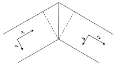
Figure 1: Schematic diagram of a 120^∘ junction, illustrating the coordinate systems for the two ribbons [$(x_{1},y_{1})$ and $(x_{2},y_{2})$]. The surface at which the two nanoribbons are joined is the solid vertical line.

we shall see that the in the zero energy limit, incoming and outgoing modes can be matched up perfectly at the junction, so that at low energies the electrons are maximally transmitted. By contrast, passage through a short length of zigzag ribbon (Fig. 2)

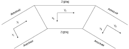
Figure 2: Schematic diagram of a 120^∘ armchair junction, in which electrons pass through a length of zigzag ribbon. Coordinates for the three sections illustrated. Wavefunctions must be matched along the two solid lines connecting the armchair ribbons to the zigzag ribbon.

involves intermediate transverse states that are strongly localized to the edges, which become orthogonal to those in the armchair leads very close to zero energy. This implies blocked transmission in a narrow range of energies near zero. Transmission through an equilateral triangle with two attached armchair leads may be viewed as a special case of this class of geometries.

A closely related geometry is transmission through an equilateral triangle with three leads. Here the system may be constructed from three appropriately cut armchair leads as illustrated in Fig. 3. As we will show in detail for this case, rapid oscillation of the fast component of the wavefunction makes the transmission very sensitive to the precise way in which these armchair leads are connected to the triangle, so that one may obtain either large or vanishingly small conductance in the low energy limit. This sensitivity to the geometry is ubiquitous for such graphene nanostructures, suggesting that a wide variety of conductance properties can in principle be engineered into very similar geometries.

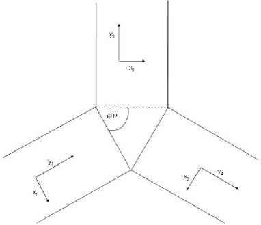
Figure 3: Schematic diagram of an equilateral triangle with three armchair leads, in which the triangle is taken as an “endcap” for the vertical lead. Coordinates for the three sections illustrated. Wavefunctions must be matched along the two solid lines of the triangle.

The SMA thus leads one to expect qualitatively different conductances for 120^∘ armchair junctions at low energies, depending on precisely how they are joined. We have tested these expectations using a tight-binding model datta for the ribbons and the regions joining them. Again, the simplest case is the 120^∘ junction between two armchair nanoribbons. An example of a specific connecting geometry and its associated low-energy conductance, computed in a tight-binding model for ribbons of conducting width, is illustrated in Fig. 4. In agreement with the SMA result, one obtains almost perfect transmission at low energies, nearly to the bottom of the first excited transverse subband energy.

\psfrag{xlabel}[0.7]{$E_{F}/E_{e}$}\psfrag{ylabel}[b][cl][0.7]{G $(e^{2}/h)$}\includegraphics[width=113.81102pt]{120Bend_AC_N=5.eps}

(a) $N$=5

\psfrag{xlabel}[0.7]{$E_{F}/E_{e}$}\psfrag{ylabel}[b][cl][0.7]{G $(e^{2}/h)$}\includegraphics[width=113.81102pt]{120Bend_AC_N=8.eps}

(b) $N$=8

\psfrag{xlabel}[0.7]{$E_{F}/E_{e}$}\psfrag{ylabel}[b][cl][0.7]{G $(e^{2}/h)$}\includegraphics[width=113.81102pt]{120Bend_AC_N=11.eps}

(c) $N$=11

\psfrag{xlabel}[0.7]{$E_{F}/E_{e}$}\psfrag{ylabel}[b][cl][0.7]{G $(e^{2}/h)$}\includegraphics[width=113.81102pt]{120Bend_AC_N=8_Diagram.eps}

(d) Geometry for $N=8$

Figure 4: Conductance per spin of 120-degree bends in armchair nanoribbons having N transverse channels. Geometry for $N$=8 illustrated in (d).

Fig. 5 illustrates a typical result for two leads joined through an equilateral triangle. As suggested by the SMA, the conductance is now suppressed near zero energy, but only over a very narrow range. Tight-binding studies of analogous geometries in which armchair leads are connected by short zigzag ribbons give similar results at low energies. One may also compute the conductance through 120^∘ when a third lead is added to the equilateral triangle. The results of such calculations are illustrated in Figs. 6 and 7. In the former case, for which the leads are attached to the triangle at their widest cross-sectional widths, one finds a highly suppressed conductance at low energy. The latter case has the leads attached to the triangle at their narrow cross-section, and the resulting conductance is large at low energy. We shall see both these results may be understood from the SMA, as special cases of the geometry illustrated in Fig. 3. Thus, the mode-matching procedure appears to offer a useful framework for understanding conductance in such geometries.

\psfrag{xlabel}[0.7]{$E_{F}/E_{e}$}\psfrag{ylabel}[b][cl][0.7]{G $(e^{2}/h)$}\includegraphics[width=113.81102pt]{Triangle_2Lead_AC_N=8.eps}

(a) $N$=8

\psfrag{xlabel}[0.7]{$E_{F}/E_{e}$}\psfrag{ylabel}[b][cl][0.7]{G $(e^{2}/h)$}\includegraphics[width=113.81102pt]{Triangle_2Lead_AC_N=11.eps}

(b) $N$=11

\psfrag{xlabel}[0.7]{$E_{F}/E_{e}$}\psfrag{ylabel}[b][cl][0.7]{G $(e^{2}/h)$}\includegraphics[width=113.81102pt]{Triangle_2Lead_AC_N=14.eps}

(c) $N$=14

\psfrag{xlabel}[0.7]{$E_{F}/E_{e}$}\psfrag{ylabel}[b][cl][0.7]{G $(e^{2}/h)$}\includegraphics[width=113.81102pt]{Triangle_2Lead_AC_N=8_Diagram.eps}

(d) Geometry for $N=8$

Figure 5: Conductance per spin of triangles with 2 armchair nanoribbons leads having N transverse channels. Geometry for $N$=8 illustrated in (d).

\psfrag{xlabel}[0.7]{$E_{F}/E_{e}$}\psfrag{ylabel}[b][cl][0.7]{G $(e^{2}/h)$}\includegraphics[width=113.81102pt]{Triangle_3Lead_AC_N=5.eps}

(a) $N$=5

\psfrag{xlabel}[0.7]{$E_{F}/E_{e}$}\psfrag{ylabel}[b][cl][0.7]{G $(e^{2}/h)$}\includegraphics[width=113.81102pt]{Triangle_3Lead_AC_N=8.eps}

(b) $N$=8

\psfrag{xlabel}[0.7]{$E_{F}/E_{e}$}\psfrag{ylabel}[b][cl][0.7]{G $(e^{2}/h)$}\includegraphics[width=113.81102pt]{Triangle_3Lead_AC_N=11.eps}

(c) $N$=11

\psfrag{xlabel}[0.7]{$E_{F}/E_{e}$}\psfrag{ylabel}[b][cl][0.7]{G $(e^{2}/h)$}\includegraphics[width=113.81102pt]{Triangle_3Lead_AC_N=8_Diagram.eps}

(d) Geometry for $N=8$

Figure 6: Conductance per spin of triangles with 3 armchair nanoribbon leads having N transverse channels, with ribbons connecting to the triangle along their wider cross-section. Geometry for $N$=8 illustrated in (d).

\psfrag{xlabel}[0.7]{$E_{F}/E_{e}$}\psfrag{ylabel}[b][cl][0.7]{G $(e^{2}/h)$}\includegraphics[width=113.81102pt]{Triangle_3Lead_AC_1point_N=5.eps}

(a) $N$=5

\psfrag{xlabel}[0.7]{$E_{F}/E_{e}$}\psfrag{ylabel}[b][cl][0.7]{G $(e^{2}/h)$}\includegraphics[width=113.81102pt]{Triangle_3Lead_AC_1point_N=8.eps}

(b) $N$=8

\psfrag{xlabel}[0.7]{$E_{F}/E_{e}$}\psfrag{ylabel}[b][cl][0.7]{G $(e^{2}/h)$}\includegraphics[width=113.81102pt]{Triangle_3Lead_AC_1point_N=11.eps}

(c) $N$=11

\psfrag{xlabel}[0.7]{$E_{F}/E_{e}$}\psfrag{ylabel}[b][cl][0.7]{G $(e^{2}/h)$}\includegraphics[width=113.81102pt]{Triangle_3Lead_AC_1point_N=8_Diagram.eps}

(d) Geometry for $N=8$

Figure 7: Conductance per spin of triangles with 3 armchair nanoribbon leads having N transverse channels, with ribbons connecting to the triangle along their narrower cross-section. Geometry for $N$=8 illustrated in (d).

The tight-binding calculations also allow us to examine the conductance at higher energies, as well as to consider other geometries. Here we summarize a few results from such studies, and give further details later on. (1) Transmission studies through hexagons with armchair leads reveal low-energy conductances that are also suppressed at low energies for 120^∘ transmission. However, in this case the suppression is quite dramatic throughout the lowest subband. Conductances per spin through 60^∘ and 180^∘ is a finite fraction of $e^{2}/h$ in the lowest subband. (2) At higher energies, we find in all of the geometries considered that the transmission as a function of energy approximately follows the density of states for bulk graphene, provided the ribbon widths are large enough. However, very close to the energy of the van Hove singularity we find a strong suppression or enhancement of the conductance depending on the angle between the leads. (3) 120^∘ zigzag ribbon junctions have a more complicated evolution with increasing ribbon width than their armchair cousins. Most notably, very close to zero energy the conductance oscillates between large and small values as the ribbon width is incremented by a single unit, reminiscent of recent results for $p-n$ junctions of zigzag ribbons akhmerov .

The remainder of this article is organized as follows. In Section II, we discuss the mode matching analysis in more detail, and explain how the SMA leads to the expectations described above. Section III is devoted to describing the numerical methods used to compute the conductance through the various geometries in the tight-binding model. In Section IV we provide further details of our numerical results. Finally, we conclude in Section V with a summary of our results.

II Mode-Matching Analysis

The conduction properties of electron systems in which current is injected into and removed from a region with a defined shape and potential, through infinite leads with known cross-section, can be understood by exploiting their analogy with electromagnetic waveguides londergan . A conceptually simple approach to their analysis is to divide the system into components where the wavefunctions may be computed with appropriate boundary conditions, and then “stitch” the wavefunctions together at the boundaries by matching their amplitudes and, in the case of wavefunctions controlled by the Schroedinger equation, their derivatives. Such calculations are made analytically tractable by employing the single-mode approximation (SMA), in which only the lowest subband of the external leads is retained, which produces qualitatively and often quantitatively good results provided one works away from scattering resonances of the system londergan . A similar strategy may be employed to understand our low energy numerical results for systems with armchair leads.

The simplest case to consider is the 120^∘ junction between two armchair ribbons illustrated in Fig. 1. The geometry is divided into regions 1 and 2 with corresponding wavefunctions $\psi^{(1)}$ and $\psi^{(2)}$ and coordinate systems $(x_{1},y_{1})$, $(x_{2},y_{2})$. At low energies one may write down approximate forms for the ribbon eigenstates brey1 . For momentum ${\bf p}$ these have the form

$$\psi^{(i)}_{p_{x},p_{y}}(x_{i},y_{i})={1\over{\sqrt{2W}}}\left\{\left(\begin{array}[]{c}1\\ \frac{p_{x}+ip_{y}}{p}\end{array}\right)e^{i{\bf K}\cdot{\bf r_{i}}}e^{ip_{x}x_{i}}-\left(\begin{array}[]{c}1\\ \frac{p_{x}+ip_{y}}{p}\end{array}\right)e^{i{\bf K}^{\prime}\cdot{\bf r}_{i}}e^{-ip_{x}x_{i}}\right\}e^{ip_{y}y_{i}},$$ (1)

where the upper (lower) entry represents the amplitude on the $A$ ($B$) sublattice, $W$ is the ribbon width, the ${\bf r}_{i}=(x_{i},y_{i})$ represent the positions of lattice points on the two ribbons, ${\bf K}=(-{{4\pi}\over{3a}},0)$, ${\bf K}^{\prime}=({{4\pi}\over{3a}},0)$, and $a$ is the lattice constant. The value of $p_{x}$ must be chosen such that the total amplitude at the edges of the ribbons vanishes, hence $p_{x}\rightarrow p_{n}$ comes in quantized values brey1 . For metallic ribbons, the lowest subband satisfies $p_{n=0}=0$. These wavefunctions have energy $\varepsilon=v_{F}|{\bf p}|$, where $v_{F}$ is the speed of electrons near the Dirac points. Due to particle-hole symmetry, we restrict our analysis to $\varepsilon\geq 0$, setting $\varepsilon=E_{F}$ for the determination of the conductance at zero temperature.

A general wavefunction in which current is injected only from the left in the lowest subband ($0<\varepsilon<v_{F}p_{1}$) may be written in the form

$$\psi^{(1)} = A_{0}\psi_{p_{n}=0,p_{y}}^{(1)}+\sum_{n}B^{(1)}_{n}\psi_{p_{n},-p_{y}}^{(1)}$$ (2)

$$\psi^{(2)} = \sum_{n}B^{(2)}_{n}\psi_{p_{n},p_{y}}^{(2)}.$$ (3)

In this expansion, it is implicitly understood that for modes where $v_{F}p_{n}>\varepsilon$, one replaces $ip_{y}$ with $\pm\kappa_{y}$ in Eq. 1 such that the wavefunctions appearing in Eqs. 2 and 3 are evanescent as one moves away from the junction. The $B^{(i)}$ coefficients are determined in terms of $A_{0}$ by matching the wavefunctions, for both sublattices, on the solid line shown in Fig. 1. The conductance per spin is then given by $G={{e^{2}}\over h}(|B_{0}^{(2)}|^{2}/|A_{0}|^{2}).$

Figure 8: Diagram detailing the joining surface between leads for the simple 120^∘ bend, as well as the labelling scheme for $x$ and $x^{\prime}$ coordinates. Matching the wavefunction on the dark circles and triangles accounts for current continuity across the joining surface.

To carry out this procedure, one must first specify a set of matching conditions at the joining surface that guarantees continuity of the wavefunctions and the current across the junction. One possible choice is illustrated in Fig. 8, where it is now convenient to change notation slightly and refer to wavefunctions $\psi,\psi^{\prime}$ and coordinates $(x,y),(x^{\prime},y^{\prime})$ in regions 1 and 2, respectively. Equating $\psi$ to $\psi^{\prime}$ on the joining line (open and closed circles) guarantees continuity of the wavefunctions. Matching currents across these junction points can be more complicated because this in general involves products of wavefunctions on either side of a bond. However we can greatly simplify the latter matching condition by anticipating the SMA, for which we will use the wavefunctions of Eq. 1, which vanish on the open circles in Fig. 8 for the lowest subband. Thus one only need match the currents on the bonds connecting the closed circles to the triangles. This may be accomplished straightforwardly by matching the wavefunctions on the triangles as well. We focus on the zero energy transmission and take the $p_{y}\rightarrow 0$ limit. The resulting matching conditions may now be written explicitly in the form

$$\begin{split}&\psi^{(A)}_{0,0}(x=1,y)=\psi^{(B)\prime}_{0,0}(x^{\prime}=1^{\prime},y^{\prime}),\\ &\quad\psi^{(B)}_{0,0}(x=2,y)=\psi^{(A)\prime}_{0,0}(x^{\prime}=1^{\prime},y^{\prime}),\\ &\qquad\psi^{(B)}_{0,0}(x=3,y)=\psi^{(A)\prime}_{0,0}(x^{\prime}=3^{\prime},y^{\prime})\\ &\psi^{(A)}_{0,0}(x=4,y)=\psi^{(B)\prime}_{0,0}(x^{\prime}=4^{\prime},y^{\prime}),\\ &\quad\psi^{(B)}_{0,0}(x=5,y)=\psi^{(A)\prime}_{0,0}(x^{\prime}=4^{\prime},y^{\prime}),\\ &\qquad\psi^{(B)}_{0,0}(x=6,y)=\psi^{(A)\prime}_{0,0}(x^{\prime}=6^{\prime},y^{\prime})\\ &\psi^{(A)}_{0,0}(x=7,y)=\psi^{(B)\prime}_{0,0}(x^{\prime}=7^{\prime},y^{\prime}),\\ &\quad\psi^{(B)}_{0,0}(x=8,y)=\psi^{(A)\prime}_{0,0}(x^{\prime}=7^{\prime},y^{\prime}),\\ &\qquad\psi^{(B)}_{0,0}(x=9,y)=\psi^{(A)\prime}_{0,0}(x^{\prime}=9^{\prime},y^{\prime})\\ &\qquad\qquad\qquad\qquad\vdots\end{split}$$ (4)

where the $x$ and $x^{\prime}$ labels are defined in Fig. 8. Simple phase factors may be added to these matching conditions to generalize them for the case $p_{y}\neq 0$. Note that in writing these equations we have equated $A$ sites of the left lead with $B$ sites of the right. This may be understood if one constructs the junction by starting with a single ribbon, excises an equilateral triangular region from the center, and joins the two resulting ribbons to form the junction. In doing this one finds that at the junction, $A$ sites are indeed matched up to $B$ sites. Note that no explicit interchange of the K and ${\bf K^{\prime}}$ valleys is needed (as is the case in $60^{\circ}$ rotations) because the real space coordinate system has also been rotated.

Eqs. 4 are a realization of setting Eq. 2 to Eq. 3 on the joining surface. To proceed, we wish to represent the wavefunctions on the matching points in an expansion in terms of wavefunctions of the form in Eq. 1. Formally, this is accomplished by multiplying these equations by $\psi^{(2)*}_{p_{n}^{\prime},p_{y}^{\prime}}(x,y)$, and then integrating $(x,y)$ on the joining surface, i.e., summing over the points where the wavefunctions have been matched. (Note $p_{y}^{\prime}$ is chosen such that $v_{F}^{2}(p_{n}^{\prime 2}+p_{y}^{\prime 2})=\varepsilon^{2}$.) This results in a set of equations relating the $A_{0}$ and $B^{(i)}$ amplitudes. A second set of equations may be generated by multiplying the matching equation by $\psi^{(1)*}_{p_{n}^{\prime},p_{y}^{\prime}}(x,y)$ and integrating on the joining surface. The two sets form an in principle infinite dimensional matrix equation that relates the $B^{(i)}$ coefficients to $A_{0}$.

Carrying out this procedure is vastly simplified by adopting the SMA, in which only the lowest transverse mode, $p_{n}=0$, is retained in the matrix equation londergan . To demonstrate the perfect transmission at low energy in the junction illustrated in Fig. 1, it is convenient to consider the reflection amplitude in the SMA. This is proportional to the integral

$$M_{0,0}(p_{y})\equiv\int d\lambda\,\,\psi^{(1)*}_{0,-p_{y}}(x(\lambda),y(\lambda))\,\psi^{(1)}_{0,p_{y}}(x(\lambda),y(\lambda)),$$ (5)

where $\lambda$ parameterizes the joining surface. Note that in the limit $p_{y}\rightarrow 0$, there is no actual $y$ ($y^{\prime}$) dependence in $\psi^{(\mu)}_{0,0}(x,y)$ ($\psi^{(\mu)\prime}_{0,0}(x^{\prime},y^{\prime})$). From Fig. 8 one may see that the positions denoted as $x(^{\prime})=n(^{\prime})$ demarcate increments of length $a/2$. The meaning of the formal expression (Eq. 5), using Eq. 1, then takes the form

$$M_{0,0}(p_{y}=0) \propto \sum_{n}\Biggl{\{}\left|\exp\left[-i\frac{2\pi}{3}\left({3\over 2}n+{1\over 2}\right)\right]-\exp\left[i\frac{2\pi}{3}\left({3\over 2}n+{1\over 2}\right)\right]\right|^{2}$$ (6)

$$- \left|\exp\left[-i\frac{2\pi}{3}\left({3\over 2}n+{1}\right)\right]-\exp\left[i\frac{2\pi}{3}\left({3\over 2}n+{1}\right)\right]\right|^{2}$$ (7)

$$+ \left|\exp\left[-i\frac{2\pi}{3}\left({3\over 2}n+{3\over 2}\right)\right]-\exp\left[i\frac{2\pi}{3}\left({3\over 2}n+{3\over 2}\right)\right]\right|^{2}=0.$$ (8)

That $M_{0,0}(p_{y})$ vanishes in the limit $p_{y}\rightarrow 0$ indicates an absence of backscattering as $\varepsilon\rightarrow 0$, and hence perfect transmission in this limit. One may also compute the corresponding overlap on the joining surface for transmission and confirm that it has a magnitude of unity. Deviations from this are of order $(p_{y}W)^{2}$, so that these become significant when $p_{y}\sim 1/W$, which occurs at an energy of the same order as the bottom of the first excited subband. Thus for energies well below this, we expect the transmission to be very close to unity. This behavior is confirmed by the tight-binding calculations.

This behavior seems dramatically different than the naïve expectation discussed in the Introduction, that the interchange of the K and ${\bf K}^{\prime}$ valleys might lead one to expect a 60^∘ deflection of the electron trajectory to be suppressed. The mode matching procedure however demonstrates that only the overlap on the joining surface need be considered, and because this involves a small subset of lattice points, destructive interference between the rapidly oscillating parts of the wavefunction may not be realized.

A second example of this procedure may be considered for the geometry illustrated in Fig. 2, in which two armchair leads are joined at the two solid lines to a short length of zigzag nanoribbon. Traversal through the equilateral triangle with two leads may be thought of as a special case of this geometry, with the shortest possible zigzag ribbon. Approximate wavefunctions $\Phi_{p_{n},p_{y}}^{(3)}(x_{3},y_{3})$ for the zigzag ribbon region may be developed brey1 . These are more complicated than the armchair forms, in that both $p_{n}$ and $p_{y}$ vary as $\varepsilon$ varies, so that the transverse wavefunctions vary with $\varepsilon$ even within a single subband. At energies close to zero, this variation becomes quite pronounced in that the wavefunctions become highly localized at the zigzag ribbon surfaces Fujita_1996 .

One may develop an explicit expression for the transmission amplitude for this geometry, within the single mode approximation, in terms of the overlap integrals on the two junctions fertig_unpub . The result is proportional to the product of the overlap integrals on each of the joining surfaces, $N^{(i)}_{0,0}(p_{y},p_{y}^{\prime})$, with

$$N^{(1)}_{0,0}(p_{y},p_{y}^{\prime}) = \int d\lambda_{1}\psi^{(1)*}_{0,p_{y}}(x(\lambda_{1}),y(\lambda_{1}))\Phi_{p_{0},p_{y}^{\prime}}^{(3)}(x(\lambda_{1}),y(\lambda_{1}))$$ (9)

$$N^{(2)}_{0,0}(p_{y},p_{y}^{\prime}) = \int d\lambda_{2}\Phi_{p_{0},p_{y}^{\prime}}^{(3)*}(x(\lambda_{2}),y(\lambda_{2}))\psi^{(2)}_{0,p_{y}}(x(\lambda_{2}),y(\lambda_{2})).$$ (10)

In these integrals, $\lambda_{1}$ and $\lambda_{2}$ parameterize the left and right surfaces in Fig. 2, $\pm p_{0}(\varepsilon)$ is the transverse momentum from which the lowest zigzag transverse state is made up brey1 ; com2 , and $\varepsilon^{2}=v_{F}^{2}p_{y}^{2}=v_{F}^{2}(p_{0}^{2}+p_{y}^{\prime 2})$. The important observation in this case is that, at low energy, the states of the zigzag ribbon $\Phi$ become confined to the surfaces, with a length scale $\xi(\varepsilon)$ which vanishes rapidly at low energy in the continuum description brey1 . Since the lowest transverse state of the armchair ribbon remains spread throughout the ribbon cross-section, one may see $N^{(i)}_{0,0}\sim\sqrt{\xi(\varepsilon)/W}$, and the resulting conductance will behave as $G\sim[\xi(\varepsilon)/W]^{2}$. This means the conductance per spin is is suppressed near zero energy, but can rise to a value of order $e^{2}/h$ once $\varepsilon$ is above the range of energies where zigzag ribbons support surface states. The resulting conductance is suppressed in a narrow range near zero energy.

As a final example, we consider the three lead equilateral triangle geometry. The SMA has a form identical to the case of the zigzag ribbon described above, with the overlap integrals now performed on surfaces joining armchair ribbons. Unlike the above two examples, the surface is oriented at different angles with respect to the cross-sections of the two ribbons, as illustrated in Fig. 3. In this case the two integrals $\tilde{N}^{(1,2)}_{0,0}$ whose product is proportional to the transmission amplitude involve a product of wavefunctions whose fast components vary at different rates as one moves along the joining surface. The resulting overlaps are very sensitive to the precise way in which the leads are joined to the triangle.

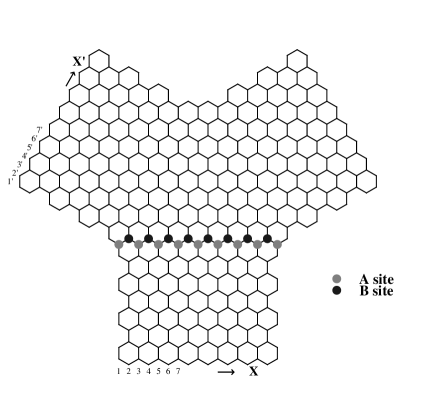
Figure 9: Diagram detailing the joining surface between the lower lead and the upper left lead, for an equilateral triangle with three leads, and the leads attached to the triangle at the wider point in their cross-section.

Fig. 9 details a joining surface for the geometry of Fig. 6. Note in this case that the ribbons are joined along zigzag edges, so that the matching of both wavefunctions and currents is easily accomplished. Denoting the wavefunction in the lower lead by $\psi^{(\mu)}_{0,p_{y}}(x,y)$ and the one in the upper left lead by $\psi^{(\mu)\prime}_{0,p_{y}}(x^{\prime},y^{\prime})$, with $\mu=A,B$, we find the matching conditions for $p_{y}=0$ to have the form

$$\begin{array}[]{cc}\psi^{(A)}_{0,0}(x=1,y)=\psi^{(A)\prime}_{0,0}(x^{\prime}=1^{\prime},y^{\prime})&\quad,\quad\psi^{(B)}_{0,0}(x=2,y)=\psi^{(B)\prime}_{0,0}(x^{\prime}=2^{\prime},y^{\prime})\\ \psi^{(A)}_{0,0}(x=3,y)=\psi^{(A)\prime}_{0,0}(x^{\prime}=2^{\prime},y^{\prime})&\quad,\quad\psi^{(B)}_{0,0}(x=4,y)=\psi^{(B)\prime}_{0,0}(x^{\prime}=3^{\prime},y^{\prime})\\ \psi^{(A)}_{0,0}(x=5,y)=\psi^{(A)\prime}_{0,0}(x^{\prime}=3^{\prime},y^{\prime})&\quad,\quad\psi^{(B)}_{0,0}(x=6,y)=\psi^{(B)\prime}_{0,0}(x^{\prime}=4^{\prime},y^{\prime})\\ \cdot&\quad\quad\cdot\\ \cdot&\quad\quad\cdot\\ \cdot&\quad\quad\cdot\\ \end{array}$$ (11)

Again, for $p_{y}=0$ there is no actual $y$ ($y^{\prime}$) dependence in $\psi^{(\mu)}_{0,0}(x,y)$ ($\psi^{(\mu)\prime}_{0,0}(x^{\prime},y^{\prime})$). The overlap between the incoming state from the bottom lead and the outgoing state from the upper left lead, using Eq. 1, has the form

$$\tilde{N}^{(1)}_{0,0} \sim {1\over W}\sum_{n}\Biggl{\{}\left[\exp\left(-i\frac{2\pi n}{3}\right)-\exp\left(i\frac{2\pi n}{3}\right)\right]\left[\exp\left(i\frac{4\pi}{3}(n+{1\over 2})\right)-\exp\left(-i\frac{4\pi}{3}(n+{1\over 2})\right)\right]$$ (12)

$$- \left[\exp\left(-i\frac{2\pi}{3}(n+1)\right)-\exp\left(i\frac{2\pi}{3}(n+1)\right)\right]\left[\exp\left(i\frac{4\pi}{3}n\right)-\exp\left(-i\frac{4\pi}{3}n\right)\right]\Biggr{\}}.$$

The upper line in Eq. 12 is due to the overlap of the wavefunctions on the $A$ sites, while the lower line comes from the $B$ sites. Multiplying out the square brackets generates terms which are either independent of the integer $n$ or oscillate in $n$ with period 3. One finds that the non-oscillating terms from the upper and lower lines precisely cancel. The remaining rapidly oscillating terms vanish in the sum provided the maximum value of $n$ is a multiple of 3, and in any case give vanishing contribution as the ribbons become wide ($W\rightarrow\infty$). The cancellation of the non-oscillating terms indicates a complete destructive interference between incoming and outgoing waves for the two arms of the triangle at low energy, as one might have naïvely supposed. With no overlap at the joining surface, the conductance should vanish at zero energy.

The other simple geometry for joining the ribbons to the triangle is detailed in Fig. 10. In this case the matching conditions take the form

$$\begin{array}[]{cc}\psi^{(A)}_{0,0}(x=1,y)=\psi^{(A)\prime}_{0,0}(x^{\prime}=1^{\prime},y^{\prime})&\quad,\quad\psi^{(B)}_{0,0}(x=2,y)=\psi^{(B)\prime}_{0,0}(x^{\prime}=1^{\prime},y^{\prime})\\ \psi^{(A)}_{0,0}(x=3,y)=\psi^{(A)\prime}_{0,0}(x^{\prime}=2^{\prime},y^{\prime})&\quad,\quad\psi^{(B)}_{0,0}(x=4,y)=\psi^{(B)\prime}_{0,0}(x^{\prime}=2^{\prime},y^{\prime})\\ \psi^{(A)}_{0,0}(x=5,y)=\psi^{(A)\prime}_{0,0}(x^{\prime}=3^{\prime},y^{\prime})&\quad,\quad\psi^{(B)}_{0,0}(x=6,y)=\psi^{(B)\prime}_{0,0}(x^{\prime}=3^{\prime},y^{\prime})\\ \cdot&\quad\quad\cdot\\ \cdot&\quad\quad\cdot\\ \cdot&\quad\quad\cdot\\ \end{array}$$ (13)

and the corresponding overlap sum is now

$$\tilde{N}^{(1)}_{0,0} \sim {1\over W}\sum_{n}\Biggl{\{}\left[\exp\left(-i\frac{2\pi n}{3}\right)-\exp\left(i\frac{2\pi n}{3}\right)\right]\left[\exp\left(i\frac{4\pi}{3}(n+{1\over 2})\right)-\exp\left(-i\frac{4\pi}{3}(n+{1\over 2})\right)\right]$$ (14)

$$- \left[\exp\left(-i\frac{2\pi}{3}n\right)-\exp\left(i\frac{2\pi}{3}n\right)\right]\left[\exp\left(i\frac{4\pi}{3}n\right)-\exp\left(-i\frac{4\pi}{3}n\right)\right]\Biggr{\}}$$

$$= {1\over W}\sum_{n}\left[-2\cos\left({{2\pi}\over 3}\right)+2+({\rm~{}oscillating~{}terms})\right].$$

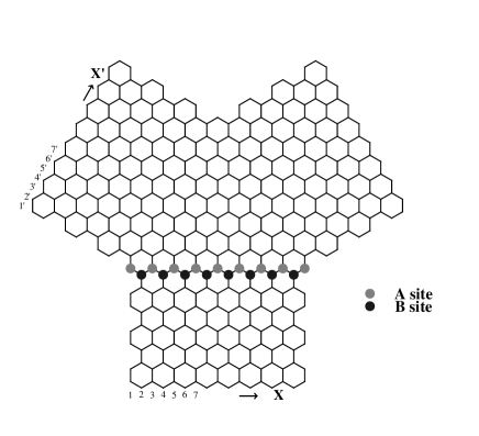
Figure 10: Diagram detailing the joining surface between the lower lead and the upper left lead, for an equilateral triangle with three leads, and the leads attached to the triangle at the narrower point in their cross-section.

We see the slight shift in positions of the $B$ sites where the wavefunctions are matched in Eq. 13 leads to an extra phase factor, such that the $A$ and $B$ overlaps no longer cancel. Thus $\tilde{N}^{(1)}_{0,0}$ is relatively large in this case, and we expect a correspondingly large transmission.

We next turn to our numerical studies, which, as discussed in the Introduction, essentially confirm the expectations of the SMA.

III Model and Numerical Method

Our calculations are based on a simple tight-binding model of graphene, in which only nearest neighbor hopping is included. Formally the Hamiltonian may be written as

$$H=-t\sum_{\{{\bf R}_{i}{\bf R}_{j}\}}\left(\left|{\bf R}_{i}\right>\left<{\bf R}_{j}\right|+\left|{\bf R}_{j}\right>\left<{\bf R}_{i}\right|\right).$$ (15)

Here $t$ is the nearest-neighbor hopping matrix element and $\{{\bf R}_{i}{\bf R}_{j}\}$ denotes bonds on a honeycomb lattice with boundaries defined by the polygon of interest and/or the attached leads. For the purposes of this section only we use the energy unit $t=1$. An example of a hexagonal scattering region with attached leads is illustrated in Fig. 11. We consider only armchair and zigzag nanoribbons for our leads, although other periodic edges may be considered within our method. We wish to calculate conductances through various pairs of leads in this geometry. Below we discuss the procedures used to evaluate the conductance per spin $G$ from Green’s functions of the Hamiltonian $H$, under the assumption of time-reversal symmetry.

Conceptually, we divide the lattice into three regions: a central region $C$, a “left” lead $L$ and a “right” lead $R$, as illustrated in Fig. 12 for the case of armchair nanoribbon leads. We compute the conductance between the leads $L$ and $R$, and any remaining leads in the geometry are considered part of the central region $C$.

Figure 11: Hexagon with 6 leads

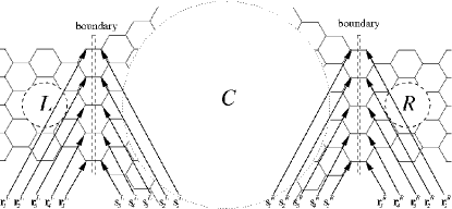
Figure 12: Conceptual division of the geometry into regions $C$, $L$, and $R$, illustrating the lattice point labeling scheme at the boundaries, which are denoted by pairs of dashed lines. This example is a symmetric armchair ribbon with $N=4$, and the boundary is chosen such that $Q=5$.

Conductance at zero temperature is computed as a linear response using the Kubo formula mahan , which relates conductivity to a current-current correlation function. For the two-lead conduction problem, the relevant current operators correspond physically to the total current in the region $L$ flowing in the incoming direction and the total current in the region $R$ flowing in the outgoing direction. We denote these operators as $\hat{J}_{L}$ and $\hat{J}_{R}$, whose precise definition we elucidate below. Charge conservation implies that the current flux down a given lead in a time-independent, steady state is the same regardless of where in the lead it is “measured”. For our purposes, it is most convenient to “measure” the current precisely at the two boundaries where the the respective leads join the central region. These boundaries are each illustrated in Fig. 12 as a pair of dashed lines.

These considerations motivate the following definitions: we label the lattice points immediately to either side of this boundary as ${\bf r}_{\mu}^{L(R)}$ for lattice points belonging to region $L(R)$ and ${\bf s}_{\mu}^{L(R)}$ for those belonging to the central region. Here $\mu$ runs over integers 1 to $Q$, where $Q$ is the number of bonds traversing the boundary. Typically $Q$ is the same as the number of channels $N$, but $Q>N$ is possible in certain configurations. This labeling scheme is illustrated in Fig. 12. The current operators may be explicitly defined as

$$\hat{J}_{L(R)}\equiv+i(-i)\mathop{\sum_{\mu=1}^{Q}}\left(\left|{\bf r}_{\mu}^{L(R)}\right>\left<{\bf s}_{\mu}^{L(R)}\right|-\left|{\bf s}_{\mu}^{L(R)}\right>\left<{\bf r}_{\mu}^{L(R)}\right|\right)$$ (16)

The Kubo formula for conductivity leads to the well-known fisher transmission formula for the conductance per spin

$$G=\frac{e^{2}}{2h}{\rm Tr}(\hat{t}_{LR}^{\dagger}\hat{t}_{LR}+\hat{t}_{RL}^{\dagger}\hat{t}_{RL})$$ (17)

where $\hat{t}_{LR(RL)}$ is the transmission amplitude for states at the Fermi energy $E_{F}$ from the region $L$ to $R$ ($R$ to $L$) and $\hat{t}_{LR}=\hat{t}_{RL}^{\dagger}$. In our context, the Kubo formula involves the operators $\hat{J}_{L}$ and $\hat{J}_{R}$, and the resulting transmission amplitudes in (17) are $Q\times Q$ matrices.

To evaluate the transmission amplitude, the relevant retarded Green’s functions are $Q\times Q$ matrices whose components are given by

$${\mathcal{G}}[\alpha,\beta]_{\mu\nu} \equiv \left<{\bf s}_{\mu}^{\alpha}\right|(E_{F}+i\eta-H)^{-1}\left|{\bf s}_{\nu}^{\beta}\right>$$ (18)

$${\mathcal{G}}^{C}[\alpha,\beta]_{\mu\nu} \equiv \left<{\bf s}_{\mu}^{\alpha}\right|(E_{F}+i\eta-H^{C})^{-1}\left|{\bf s}_{\nu}^{\beta}\right>$$ (19)

$${\mathcal{G}}^{L}_{\mu\nu} \equiv \left<{\bf r}_{\mu}^{L}\right|(E_{F}+i\eta-H^{L})^{-1}\left|{\bf r}_{\nu}^{L}\right>$$ (20)

$${\mathcal{G}}^{R}_{\mu\nu} \equiv \left<{\bf r}_{\mu}^{R}\right|(E_{F}+i\eta-H^{R})^{-1}\left|{\bf r}_{\nu}^{R}\right>.$$ (21)

Here $H^{L}$, $H^{R}$, $H^{C}$ represent the restriction of the Hamiltonian to regions $L$, $R$, and $C$, respectively (with no hopping across the boundaries), and $\alpha$ and $\beta$ can be $L$ or $R$. Ideally, $\eta\rightarrow 0^{+}$, but for numerical calculations it is necessary to choose a small $\eta>0$ which in effect becomes the energy resolution of the computation. Our calculations are carried out with $\eta=10^{-6}t$.

With these definitions, we have, in abbreviated notation for the $Q\times Q$ matrices,

$$\hat{t}_{LR} = \hat{v}_{R}^{1/2}\hat{{\mathcal{G}}}[R,L]\hat{v}_{L}^{1/2}$$ (22)

$$\hat{v}_{L(R)} \equiv i(\hat{{\mathcal{G}}}^{L(R)}-\hat{{\mathcal{G}}}^{L(R)\dagger}).$$ (23)

Schematically, this formula shows that the transmission amplitude is given by the propagator from the left to right side of the central region, with the $\hat{v}_{L(R)}$ velocity matrices normalizing the nanoribbon states to unit flux. The problem is now reduced to computing $\hat{{\mathcal{G}}}^{L(R)}$ and $\hat{{\mathcal{G}}}^{C}$. Standard gluing formulas Sols for non-interacting Green’s functions can be used to obtain $\hat{{\mathcal{G}}}[R,L]$ from these two.

For our geometries, $\hat{{\mathcal{G}}}^{L(R)}$ is the Green’s function of a semi-infinite nanoribbon at its termination. One may directly evaluate the Green’s function of a single nanoribbon unit cell by inverting the matrix $(E_{F}+i\eta-h)$, where $h$ is its lattice Hamiltonian. We then rapidly extend from the unit cell to a nanoribbon segment of length $2^{l}$ through $l$ successive length-doubling steps via the aforementioned gluing formulas. We find that the Green’s function on one termination of the long nanoribbon segment becomes an accurate approximation for the semi-infinite ribbon when $2^{l}\sim t/\eta$. This can be verified by substituting the numerical result into a Dyson equation satisfied by the exact Green’s function. Such a Dyson equation may be easily derived for any such semi-infinite periodic structure.

For $\hat{{\mathcal{G}}}^{C}$ we first suppose that the geometry has only two leads and thus the region $C$ is finite. One approach is to perform the matrix inversion of $(E_{F}+i\eta-H^{C})$. However, significant computational savings are possible when the Green’s function is only required at the boundary Iyengar_unpublished . In the case of more than two leads, ${\mathcal{G}}^{C}$ can be found by gluing the Green’s functions for the “passive” leads in the calculation to the Green’s function of the finite scattering region. This procedure correctly accounts for current which is drained away by the extra leads.

We first tested our numerical techniques on the straightforward case of infinite nanoribbons, whose bandstructure is well-understood brey1 . Nanoribbons may be characterized by the number $N$ of conducting channels. The integer $N$ gives two related properties of the ribbon: 1) the minimum number of severed bonds required to break the ribbon into two disconnected pieces (as in Fig. 13) and 2) the maximum possible value of $G$, the conductance per spin, in units of the conductance quantum $e^{2}/h$. Armchair nanoribbons have associated with them two lines of fictive lattice points (just outside the actual ribbon edges) separated by a width $La$ (see Fig. 13) on which the wavefunction vanishes. When the ribbons possess a reflection symmetry through the center, $N=L-1$, and otherwise $N=L-1/2$. In either case, the ribbon is semiconducting (i.e. there is gap in the spectrum around zero energy) unless $\sin(4\pi L/3)=0$. Thus, symmetric armchair nanoribbons are metallic only for the series $N=2,5,8,\ldots$ and the asymmetric ribbons for $N=1,4,7,10,\ldots$. Zigzag ribbons are metallic for any value of $N$.

We have compared the conductance of these various types of ribbons as a function of $E_{F}$ with their bandstructure. We find, as expected, a contribution to $G(E_{F})$ of $e^{2}/h$ for each band present at $E_{F}$, with the exception of the flat bandsflatbands in symmetric armchair ribbons at energies $\pm t$. We also verify the linear dispersion of the metallic band in armchair nanoribbons with velocity $v_{F}=\sqrt{3}ta/2$, as well as the maximum $G$ values and metallic $N$ sequences discussed above.

Figure 13: Symmetric armchair, asymmetric armchair, and zigzag ribbons with $N=4$. Dashed line cuts through four bonds of each ribbon, the minimal number required to sever each into two disconnected pieces. Heavy vertical lines indicate rows of fictive lattice points along which the wavefunction vanishes for the armchair nanoribbons.

IV Numerical Results

IV.1 Armchair Lead Systems: $120^{\circ}$ Junctions and Triangles

Our low-energy result for the simple junction for armchair leads at low energy was discussed in the Introduction, and is illustrated in Fig. 4. One clearly sees that the tranmission is essentially perfect, with a small suppression just below the first excited subband energy. The behavior appears to be well-explained by the SMA. The $120^{\circ}$ junction also naturally occurs in an equilateral triangle with two leads, as illustrated in Fig. 5(d). As has already been explained, at low energies one finds suppression of the conductance in a narrow range around zero energy.

We discuss more fully the example of the three lead triangle geometry, illustrated in Fig. 6(d). Because of the symmetry of this geometry, the two point conductance is the same for any pair of the three leads. Fig. 14 illustrates the conductance for three different system sizes as a function of Fermi energy $E_{F}$ over the entire bandwidth. One may see that the overall shape of the conductance curve roughly tracks the density of states for bulk graphene, with peaks at the van Hove singularities $E_{F}=t$, where $t$ is the hopping matrix element. The bumps and wiggles around this are due to changes in the number of conducting channels as the Fermi energy is increased, as well as to quantum interference in the scattering region datta .

\psfrag{xlabel}[0.7]{$E_{F}/t$}\psfrag{ylabel}[b][cl][0.7]{G $(e^{2}/h)$}\includegraphics[width=113.81102pt]{Triangle_3Lead_AC_FullBand_N=5.eps}

(a) $N$=5

\psfrag{xlabel}[0.7]{$E_{F}/t$}\psfrag{ylabel}[b][cl][0.7]{G $(e^{2}/h)$}\includegraphics[width=113.81102pt]{Triangle_3Lead_AC_FullBand_N=10.eps}

(b) $N$=10

\psfrag{xlabel}[0.7]{$E_{F}/t$}\psfrag{ylabel}[b][cl][0.7]{G $(e^{2}/h)$}\includegraphics[width=113.81102pt]{Triangle_3Lead_AC_FullBand_N=15.eps}

(c) $N$=15

Figure 14: Conductance per spin through an equilateral triangle with three armchair leads of sizes (a) $N$=5, (b) $N$=10, and (c) $N$=15.

The low energy region of conductance for different system sizes may also be considered. In Fig. 15 we blow up the low-energy region for three different system sizes. The cases $N=13$ and $N=15$ as expected reveal no conduction at low energies, since there are no conducting states to carry current through the leads. The metallic state for $N=14$, by contrast, allows a finite conductance, but one may see its actual value is remarkably small at very low energy. One may examine this behavior with increasing $N$, and not surprisingly the pattern of near suppression for system sizes of the form $N=3M+2$, and complete suppression for other sizes, repeats itself. When viewed as a function of $E_{F}/E_{e}$, which fixes the position of the opening of the first excited subband as $N$ becomes large, the conductance in the lowest subband tends to a roughly parabolic shape, very small but remaining finite away from $E_{F}=0$ as $N\rightarrow\infty$. This represents the continuum limit, in which the width $W$ of the ribbons remain finite, and the lattice constant $a$ is taken to zero. The increase from zero of the conductance as the energy increases from zero is in agreement with the results of the SMA, but we note that the vanishing conductance for these widths requires the joining geometry illustrated in Fig. 9. As discussed in the Introduction, a joining geometry of the form illustrated in Fig. 10 leads to a non-vanishing conductance (Fig. 7), in agreement with the SMA analysis.

\psfrag{xlabel}[0.7]{$E_{F}/E_{e}$}\psfrag{ylabel}[b][cl][0.7]{G $(e^{2}/h)$}\includegraphics[height=71.13188pt]{Triangle_3Lead_AC_N=13.eps}

(a) $N$=13

\psfrag{xlabel}[0.7]{$E_{F}/E_{e}$}\psfrag{ylabel}[b][cl][0.7]{G $(e^{2}/h)$}\includegraphics[height=71.13188pt]{Triangle_3Lead_AC_N=14.eps}

(b) $N$=14

\psfrag{xlabel}[0.7]{$E_{F}/E_{e}$}\psfrag{ylabel}[b][cl][0.7]{G $(e^{2}/h)$}\includegraphics[height=71.13188pt]{Triangle_3Lead_AC_N=15.eps}

(c) $N$=15

Figure 15: Conductance per spin in the low energy region for an equilateral triangle with three armchair leads. (a) $N$=13, (b) $N$=14, (c) $N$=15.

IV.2 Transmission Through a Hexagon

We next consider the case of a hexagon with six attached leads, as illustrated schematically in Fig. 11. The conductance per spin is illustrated for the full bandwidth in Figs. 16, 17, and 18. Here we must specify the angle between the two leads upon which the measurement is made: Fig. 16 corresponds to a 60^∘ angle between leads, Fig. 17 to 120^∘, and Fig. 18 to 180^∘. Several remarks are in order. As in the equilateral triangle, the overall structure of the conductance follows the density of states for bulk graphene. However, as the size of the system increases it is apparent that there is a remarkably sharp suppression for transmission through 60^∘ and 180^∘, and a strong enhancement for transmission through 120^∘, at the van Hove singularity, $E_{F}/t=1$. The rapid change in resistance with respect to Fermi energy suggests that this phenomenon could in principle be useful as a transistor, although the relatively high Fermi energy where it occurs may require a large electric field to realize. Beyond this, it is also noteworthy that the overall scale of transmission through 120^∘ is significantly larger, and seems to grow more quickly with system size, than for the other two directions.

\psfrag{xlabel}[0.7]{$E_{F}/t$}\psfrag{ylabel}[b][cl][0.7]{G $(e^{2}/h)$}\includegraphics[width=113.81102pt]{Hex_6Lead_AC_FullBand_N=5_60deg.eps}

(a) $N$=5

\psfrag{xlabel}[0.7]{$E_{F}/t$}\psfrag{ylabel}[b][cl][0.7]{G $(e^{2}/h)$}\includegraphics[width=113.81102pt]{Hex_6Lead_AC_FullBand_N=15_60deg.eps}

(b) $N$=15

\psfrag{xlabel}[0.7]{$E_{F}/t$}\psfrag{ylabel}[b][cl][0.7]{G $(e^{2}/h)$}\includegraphics[width=113.81102pt]{Hex_6Lead_AC_FullBand_N=20_60deg.eps}

(c) $N$=20

Figure 16: Conductance per spin for two leads at an angle of 60^∘, through a hexagon with six armchair leads. (a) $N$=5, (b) $N$=15, (c) $N$=20.

\psfrag{xlabel}[0.7]{$E_{F}/t$}\psfrag{ylabel}[b][cl][0.7]{G $(e^{2}/h)$}\includegraphics[width=113.81102pt]{Hex_6Lead_AC_FullBand_N=5_120deg.eps}

(a) $N$=5

\psfrag{xlabel}[0.7]{$E_{F}/t$}\psfrag{ylabel}[b][cl][0.7]{G $(e^{2}/h)$}\includegraphics[width=113.81102pt]{Hex_6Lead_AC_FullBand_N=15_120deg.eps}

(b) $N$=15

\psfrag{xlabel}[0.7]{$E_{F}/t$}\psfrag{ylabel}[b][cl][0.7]{G $(e^{2}/h)$}\includegraphics[width=113.81102pt]{Hex_6Lead_AC_FullBand_N=20_120deg.eps}

(c) $N$=20

Figure 17: Conductance per spin for two leads at an angle of 120^∘, through a hexagon with six armchair leads. (a) $N$=5, (b) $N$=15, (c) $N$=20.

\psfrag{xlabel}[0.7]{$E_{F}/t$}\psfrag{ylabel}[b][cl][0.7]{G $(e^{2}/h)$}\includegraphics[width=113.81102pt]{Hex_6Lead_AC_FullBand_N=5_180deg.eps}

(a) $N$=5

\psfrag{xlabel}[0.7]{$E_{F}/t$}\psfrag{ylabel}[b][cl][0.7]{G $(e^{2}/h)$}\includegraphics[width=113.81102pt]{Hex_6Lead_AC_FullBand_N=15_180deg.eps}

(b) $N$=15

\psfrag{xlabel}[0.7]{$E_{F}/t$}\psfrag{ylabel}[b][cl][0.7]{G $(e^{2}/h)$}\includegraphics[width=113.81102pt]{Hex_6Lead_AC_FullBand_N=20_180deg.eps}

(c) $N$=20

Figure 18: Conductance per spin for two leads at an angle of 180^∘, through a hexagon with six armchair leads. (a) $N$=5, (b) $N$=15, (c) $N$=20.

The conductance at low-energy for this geometry is illustrated in Fig. 19 for $N=20$, for conductance through each of the three angles. A suppression of 120^∘ transmission is apparent, and in this case is in fact much more pronounced throughout the first subband than is the case for the equilateral triangle. Indeed, in studies of hexagons with only three or two leads, we find the 120^∘ transmission to be even more suppressed throughout the lowest subband than in the six lead case. This suggests the hexagon may be useful in three terminal devices where one may wish to employ one lead as a voltage probe without draining current flowing between other leads.

\psfrag{xlabel}[0.7]{$E_{F}/E_{e}$}\psfrag{ylabel}[b][cl][0.7]{G $(e^{2}/h)$}\includegraphics[width=113.81102pt]{Hex_6Lead_AC_N=20_lowenergy_60deg.eps}

(a) 60^∘

\psfrag{xlabel}[0.7]{$E_{F}/E_{e}$}\psfrag{ylabel}[b][cl][0.7]{G $(e^{2}/h)$}\includegraphics[width=113.81102pt]{Hex_6Lead_AC_N=20_lowenergy_120deg.eps}

(b) 120^∘

\psfrag{xlabel}[0.7]{$E_{F}/E_{e}$}\psfrag{ylabel}[b][cl][0.7]{G $(e^{2}/h)$}\includegraphics[width=113.81102pt]{Hex_6Lead_AC_N=20_lowenergy_180deg.eps}

(c) 180^∘

Figure 19: Conductance per spin for two leads at an angle of (a) 60^∘, (b) 120^∘, and (c) 180^∘ through a hexagon with six $N$=20 armchair leads.

IV.3 Zigzag Nanoribbon Junctions

We conclude this section with a summary of analogous results for a 120^∘ zigzag nanoribbon junction. Like armchair ribbons, zigzag ribbon widths may be characterized by the minimum number of broken bonds $N$ required to sever it, as illustrated in Fig. 13. Unlike armchair ribbons, zigzag ribbons are metallic for any width brey1 . At low energies the current-carrying states have an interesting chirality in that left- and right-moving states are associated with different valley indices rycerz . It should be emphasized that the association of this discrete index can only be made precise in a continuum description. All the geometries considered below may always be understood in terms of semi-infinite ribbons joined together at boundaries on the lattice scale. Because the lowest energy states of zigzag ribbons are highly confined to the edges of the system, a pure continuum description is inadequate even at the lowest energies. Similar physics has been noted recently in graphene $p-n$ junctions akhmerov .

This physics is most clearly seen in 120^∘ zigzag junctions. Fig. 20 illustrates the transmission for this geometry for ribbon widths $N$=6,7, and 8. At very low energies, there is a qualitative difference between odd and even width ribbons, with the former supporting a large conductance at zero energy and the latter a small one. Such odd-even behavior also occurs in $p-n$ junctions, and appears to be related to the fact that edges in a zigzag ribbon align when $N$ is even, but anti-align for odd $N$ akhmerov ; waka . Even at higher energies, but still within the lowest subband, the conductance as a function of energy appears to change qualitatively from one width to the next as $N$ increments by single units.

\psfrag{xlabel}[0.7]{$E_{F}/E_{e}$}\psfrag{ylabel}[b][cl][0.7]{G $(e^{2}/h)$}\includegraphics[width=113.81102pt]{120Bend_ZZ_N=6.eps}

(a) $N$=6

\psfrag{xlabel}[0.7]{$E_{F}/E_{e}$}\psfrag{ylabel}[b][cl][0.7]{G $(e^{2}/h)$}\includegraphics[width=113.81102pt]{120Bend_ZZ_N=7.eps}

(b) $N$=7

\psfrag{xlabel}[0.7]{$E_{F}/E_{e}$}\psfrag{ylabel}[b][cl][0.7]{G $(e^{2}/h)$}\includegraphics[width=113.81102pt]{120Bend_ZZ_N=8.eps}

(c) $N$=8

\psfrag{xlabel}[0.7]{$E_{F}/E_{e}$}\psfrag{ylabel}[b][cl][0.7]{G $(e^{2}/h)$}\includegraphics[width=113.81102pt]{120Bend_ZZ_N=8_Diagram.eps}

(d) Geometry for $N$=8

Figure 20: Transmission through 120^∘ bend for zigzag ribbons. (a) $N$=6, (b) $N$=7, (c) $N$=8. (d) Geometry for $N$=8.

The importance of lattice scale physics in this system is further made apparent by an examination of the local density of states at low energies. This is shown in in Fig. 21 for a junction of width $N$=6 at several energies below the first excited subband energy. At low energies, while the wavefunction is strongly maximized near the ribbon edges, the junction can attain zero or perfect conductance, as is the case in (a) and (b), respsectively. As the wavefunctions throughout the first subband intimately involve the lattice scale, any continuum description for this system is not likely to be reliable.

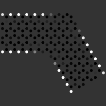
(a) $E_{F}/E_{e}$=0.016

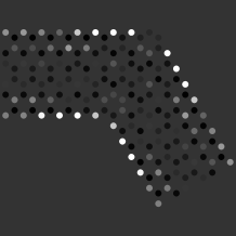
(b) $E_{F}/E_{e}$=0.16

(c) $E_{F}/E_{e}$=0.49

(d) $E_{F}/E_{e}$=0.82

Figure 21: Local density of states shown in gray scale for 120^∘ degree zigzag junction, $N=6$. Black denotes zero, and white denotes maximal LDOS. The leads modelled in the calculation extend away from the junction to infinity.

V Conclusion

In this paper we have studied the conductance of various graphene geometries in which the current in a nanoribbon is redirected through angles that are multiples of 60^∘, which can be accomplished in the honeycomb network without introducing lattice defects or changing the ribbon type. We focus on the low-energy behavior in armchair nanoribbon geometries and find a variety of behaviors, including very high transmission for a particular realization of a simple 120^∘ junction and suppressed transmission for the same angle when there is an intervening triangle. A mode-matching analysis, within the single-mode approximation (SMA), allows one to understand in a simple way many of these results. With this technique we demonstrate that the rapid oscillation of the low energy wavefunctions renders the conductance through such junctions highly sensitive to the precise way in which the ribbons are joined together. Tight-binding calculations support the conclusions of the SMA at low-energies, and further elucidate the details of the conductance at higher energies.

We also presented numerical results for conductance through other geometries. Hexagons in particular showed a dramatic suppression of conductance through $120^{\circ}$, and further supported a strong enhanced/suppressed conductance (depending on the angle between the leads) at the van Hove singularity. Zigzag nanoribbon junctions were also studied, and were found to have a richer behavior than their armchair cousins, which is likely to require a more microscopic description than is possible in a continuum model.

VI Acknowledgements

The authors thank J.P. Carini, F. Guinea and C. Tejedor for useful discussions. This work was supported by MAT2006-03741 (Spain) (LB) and by the NSF through Grant No. DMR-0704033 (HAF).

References

- (1) K.S. Novoselov et al., Science 306, 666 (2004).
- (2) A.H. Castro Neto et al., arXiv:0709.1163; V.P. Gusynin, S.G. Sharapov, and J.P. Carbotte, Int. J. Mod. Phys. 27, 4611 (2007).
- (3) T. Ando, J. Phys. Soc. Jpn. 74, 777 (2005) and N.M.R.Peres, F.Guinea and A.H.Castro-Neto, Phys.Rev.B 72, 174406 (2005) and references therein.
- (4) N.H. Shon and T. Ando, J. Phys. Soc. Jpn., 67, 2421 (1998).
- (5) L. Brey and H.A. Fertig, Phys. Rev. B 73, 195408 (2006).
- (6) L. Brey and H.A. Fertig, Phys. Rev. B 73, 235411 (2006).
- (7) F.Munoz-Rojas, J.Fernandez-Rossier, L.Brey and J.J.Palacios, PRB 77 045301 (2008).
- (8) M.Y. Han, B. Ozyilmaz, and Y.B. Zhang, and P. Kim, Phys. Rev. Lett. 98, 206805 (2007).
- (9) Z. Chen, Y.M. Lin, M.J. Roukes, and P. Avouris, cond-mat/0701599.
- (10) X. Li, X. Wang, L. Zhang, S. Lee, and H. Dai, Science 319, 1229 (2008).
- (11) S. Datta, Electronic Transport in Mesoscopic Systems, (Cambridge, New York, 1997).
- (12) A. Rycerz, J. Tworzydlo, and C.W.J. Beenakker, Nature Physics 3, 172 (2007).
- (13) J.T. Londergan, J.P. Carini, and D.P. Murdock, Binding and Scattering in Two-Dimensional Systems (Springer-Verlag, New York, 1999).
- (14) A.R. Akhmerov, J.H. Bardarson, A. Rycerz, and C.W.J. Beenakker, arXiv:0712.3233.
- (15) Note that setting the wavefunctions equal on the A and B sublattices for wavefunctions satisying the Dirac equation is essentially equivalent to matching both wavefunctions and derivatives for those satisfying the Schroedinger equation brey2 .
- (16) K.Wakabayashi and T.Aoki, Int.J.Mod.Phys.B 16 4897 (2002).
- (17) M. Fujita et al., J. Phys. Soc. Jpn. 65, 1920 (1996).
- (18) H.A. Fertig, unpublished.
- (19) Note that is actually imaginary for very low energies, where the zigzag ribbon supports surface states.
- (20) G.D. Mahan, Many-Particle Physics, (Plenum Publishers, New York, 2000).
- (21) F. Sols, M. Macucci, U. Ravaioli, and K. Hess, Jour. Appl. Phys. 66, 3892 (1989).
- (22) D.S. Fisher and P.A. Lee, Phys. Rev. B 23, 6851 (1981).
- (23) A.P. Iyengar, unpublished.
- (24) Hsiu-Hau Lin, Toshiya Hikihara, Bor-Lung Huang, Chung-Yu Mou, Xiao Hu, arXiv:cond-mat/0410654.