Soliton structures in a molecular chain model with saturation

Abstract

In the present work, we study, by means of a one-dimensional lattice model, the collective excitations corresponding to intra molecular ones of a chain like proteins. It is shown that such excitations are described by the Nonlinear Schrodinger equation with saturation. The solutions obtained here are the bell solitons, bubbles, kinks and crowdons. Since they belong to different sectors on the parametric space, the bubble condensation could give place to some important changes of face in this kind of nonlinear system. Additionally, it is shown that the limiting velocity of the solitons is the velocity of sound waves corresponding to longitudinal vibrations of molecules.

I Introduction

In the present days the research to the dynamic properties of one dimensional molecular chains have increased. The structure of a great amount of macromolecules is represented by subunits with mutually weak, slightly flexible bounds connecting them with each other. The important biological structures of this type are RNA, proteins and DNA polymer chains. The peculiarity of bio-polymers is that, they are heterogeneous, and their elementary subunits have complex structures and carry long-lived nonlinear excitations. As it is well known the propagation of energy and electrons in protein molecules is the crucial factor for maintaining the life of biological systems. So, the problem of storage and transportation of energy through protein chains arises. The energy used in biological cell comes from the energy of liberation during the process of hydrolysis of adenosinetriphosphate (ATP) molecular structures. The energy of this process is of approximately 0,42 eV (or 2250 cm^-1). Proteins consist of chains of hydrogen-bonded peptide groups, three of these chains in a helical arrangement define the $\alpha-$helix structure ev . In his seminal work, Davydov proposed an explanation of the fundamental transportation problem of energy released by hydrolysis of adenosinetriphosphate and transferred to proteins in biological systems davidov . This energy remains localized and moves along the protein chains at a reasonable rate to perform useful biological functions. It could be trapped and transported in proteins as quanta of the intra molecular C=O stretching mode, the so called amide-I vibration, with excitation energy around 1650cm^-1. The localized spatial region where the energy is trapped can propagate along the protein chain, in such a way that a soliton-like mechanism for energy transport is possible. This problem of transporting energy from one point to another inside the cell is a long-standing problem that remains of great interest.

Besides, from experimental point of view, we can also discover a lot of contributions that are directly related to a similar phenomenon in the DNA. For instance, in the experimental work on short DNA rings e.g., Refs. ring ; ring2 the kink tendency of DNA sequences were studied. In the last years the great amount of works devoted to the nonlinear dynamics of DNA shows that this area is an active field, for example theoretical proposals of wrapping DNA around the nucleosome, where kinks play a great rule, were proposed in various papers, see the Refs.agrawal ; cuevas ; chris . Concerning the $\alpha-$helical protein dynamics, some works have been dedicated to study this system including high order excitations and different molecular interactions, in the discrete and continuum level, daniel ; scott .

In this contribution we investigate soliton-like structures within the framework of a certain generalization of the Davydov’s model, considering the case of neighboring interactions as the same class before and after a peptide group. In the next section we briefly expose the modified Davydov’s model leading to the Hamiltonian that will be used in the later. Section III is devoted to derive the nonlinear cubic - quintic Schrodinger equation by a suitable transformation from the original nonlinear Schrodinger equation with saturation. The soliton structures of this equation with some specific characteristics are presented in section IV. Finally, in the last section we deliver some comments.

II Davydov’s Model.

Due to its transparency and seminal properties, Davydov‘s model continues to encourage intense work regarding the research of the nonlinear treatment of molecular systems davidov . In his pioneer works he and co-workers demonstrated that the corresponding nonlinear equations for the molecular excitation in the quantum treatment admit solitonic structures. Indeed they assumed that the energy transportation in proteins is carried out by means of transportation of amide - I vibration. In what follows we consider an infinite chain of weakly bound molecules (or groups) with a mass $M$ and a distance $R$ from each other. Internal excitations of molecules (electronic or vibrational) are characterized by an energy and an electric dipole moment $d$ directed along the chain. The internal excitation of molecules and their motion around equilibrium positions are inseparably linked.

In the case of a one-dimensional chain, only interactions between neighbor molecules are taken into consideration. Below, we follow the modeling done by Davydov and his co-workers. If the intramolecular excitation has the energy $\varepsilon$, the collective excitations of this model can be described by the Davydov’s Hamiltonian:

$$H = \sum_{n}\left[(\varepsilon-D_{n})B_{n}^{+}B_{n}-J\left(B_{n+1}^{+}B_{n}+B_{n+1}B_{n}^{+}\right)\right]$$ (1)

$$+T+U,$$

where index $n$ labels the molecule that occupies position $r_{n}$ in the chain, while $B_{n}^{+}$ y $B_{n}$ are creation and annihilation of intramolecular excitation boson operators. The quantity $J=2d^{2}R^{-3}$ characterizes the transition of intramolecular excitation due to the resonant interactions while $d$ is the electric dipolar moment. The last two terms in (1), as usual, correspond to the kinetic and potential energies of the longitudinal displacements.

When the $i$-th molecule is excited, the static interaction with neighboring molecules of this molecule changes. This is reflected by the introduction of the function $D_{n}$. The displacement $\rho_{n}$ from the equilibrium distance $R$ in the state $\mid\Psi\rangle$ is defined by the expression

$$\rho_{n}=R-(r_{n}-r_{n-1}).$$ (2)

In the state $\mid 0\rangle\;$ without intramolecular excitation, the chain has periodicity and the intermolecular distances are $R$.

Let us now consider the function $D_{n}$, which in the nearest neighbors interaction limit has the following form

$$D_{n} = \mathfrak{D}_{n}\left(\left|r_{n-1}-r_{n}\right|\right)+\mathfrak{D}_{n}\left(\left|r_{n}-r_{n+1}\right|\right)$$ (3)

$$\approx \left(1+\frac{\beta}{R}\rho_{n}+\frac{\beta\gamma}{2R^{2}}\rho_{n}^{2}\right)D,$$

where $D\equiv 2\mathfrak{D}_{n}\left(R\right),\beta,\gamma$ are parameters of the theory.

The potential energy of the molecules in the non excited chain is chosen in a harmonic approximation under the assumption that the constant spring $\omega\$is the same for all of them. In this case we can express the potential energy as

$$U=\frac{1}{2}\omega\sum\limits_{n}\rho_{n}^{2},$$

and the kinetic energy can be written as

$$T=\frac{1}{2}M\sum\limits_{n}\left(\dot{r}_{n}\right)^{2}=\frac{1}{2}M\sum\limits_{n}\left(\sum\limits_{-\infty>l\leq n}\dot{\rho}\right)^{2},$$

where dot over the letter represents temporal derivative, $\dot{\rho}\equiv\frac{d\rho}{dt}.$ According with the quantum mechanics treatment the collective interactions of interest can be described by the wave function

$$\left|\Psi\right\rangle=\sum\limits_{n}\psi_{n}\left(t\right)B_{n}^{+}\left|0\right\rangle,$$

where coefficients $\psi_{n}\left(t\right)$ are normalized as $\sum\limits_{n}\left|\psi_{n}\left(t\right)\right|^{2}=1.$ These coefficients characterize the distribution of excitations along the molecular chain, $\psi_{n}$ being the probability of finding the quantum system in the site $n$ or $\left|\psi_{n}\left(t\right)\right|^{2}$ being the density of probability of finding the excitation. The equation for determining these wave functions can be obtained from the Schrödinger equation

$$i\hbar\frac{\partial}{\partial t}\left|\Psi\right\rangle=H\left|\Psi\right\rangle,$$

that can be reduced, using the explicit form of the operator $H$, Eq. (1), the fact that the functions $B_{n}^{+}\left|0\right\rangle$ correspond to different values of $n$ and are orthogonal each other, to obtain the following system of equations

$$i\hbar\frac{\partial\psi_{n}}{\partial t} = \left[\varepsilon+T+U-\left(1+\frac{\beta}{R}\rho_{n}+\frac{\beta\gamma}{2R^{2}}\rho_{n}^{2}\right)D\right]\psi_{n}$$ (4)

$$-J\left(\psi_{n+1}+\psi_{n+1}\right).$$

The functional i.e. the hamiltonian that can be associated with this equation of motion can be written as $F=\left\langle\Psi\right|H\left|\Psi\right\rangle$

$$F = \sum\limits_{n}\left\{\left[\varepsilon+T+U-\left(1+\frac{\beta\rho_{n}}{R}+\frac{\beta\gamma\rho_{n}^{2}}{2R^{2}}\right)D\right]\psi_{n}^{\ast}\psi_{n}\right.$$

$$\left.-J\psi_{n}^{\ast}\left(\psi_{n+1}-\psi_{n-1}\right)\right\}.$$

Following Toda Toda , it is convenient to associate the displacements $\rho_{n}$ with their canonically conjugate variables $s_{n}=\frac{\partial T}{\partial\dot{\rho}_{n}}=-M\sum\limits_{l\geq n}\dot{r}_{l}$. Then the kinetic energy can be expressed in terms of these new variables as

$$T=\frac{1}{2M}\sum\limits_{n}\left(s_{n}-s_{n-1}\right)^{2}.$$

In the next section we will see the derivation for the nonlinear Schrödinger equation (NSE) with a saturation term.

III NSE equation with saturation

Now, we can derive the equation of motion for the displacements and for their canonical conjugate variables $s_{n}$, for this we consider that

$$\dot{\rho}_{n} = \frac{\partial F}{\partial s_{n}}=\frac{1}{M}\left(2s_{n}-s_{n+1}-s_{n-1}\right),$$

$$\dot{s}_{n} = -\frac{\partial F}{\partial\rho_{n}}=-\omega\rho_{n}+\frac{\beta D}{R}\left|\psi_{n}\left(t\right)\right|^{2}+\frac{\beta\gamma D}{R^{2}}\rho_{n}\left|\psi_{n}\left(t\right)\right|^{2}.$$ (5)

After eliminating the variables $s_{n}$ from the preceding system of equations, we find the equation for the displacement

$$\ddot{\rho}_{n} = -\frac{\omega}{M}\left(2\rho_{n}-\rho_{n+1}-\rho_{n-1}\right)$$ (6)

$$+\frac{\beta D}{RM}\left(2\left|\psi_{n}\right|^{2}-\left|\psi_{n+1}\right|^{2}-\left|\psi_{n-1}\right|^{2}\right)+$$

$$+\frac{\beta\gamma D}{R^{2}M}\left(2\rho_{n}\left|\psi_{n}\right|^{2}-\rho_{n+1}\left|\psi_{n+1}\right|^{2}-\rho_{n-1}\left|\psi_{n-1}\right|^{2}\right).$$

The system of equations ( 4) and (6) defines the collective excitations and deformation of a chain.

For an analytical treatment if we are interested on the distribution of excitations along the chain, we turn to the analysis in the continuum limit. For doing this, let us introduce the dimensionless variable $\xi=\frac{r}{R}$ and the continuous functions as usual $\rho\left(\xi,t\right)$ and $\psi\left(\xi,t\right)$ such that

$$\rho\left(n,t\right)=\rho_{n}\left(t\right),\;\;\;\;\;\;\;\;\;\;\;\psi\left(n,t\right)=\psi_{n}\left(t\right).$$

Expanding $\rho\left(\xi\pm 1\right)$ and $\psi\left(\xi\pm 1\right)$ in series in the standard manner

$$\rho\left(\xi\pm 1,t\right) \approx \rho\left(\xi\right)\pm\frac{\partial\rho\left(\xi,t\right)}{\partial\xi}+\frac{1}{2}\frac{\partial^{2}\rho\left(\xi,t\right)}{\partial\xi^{2}},$$

$$\psi\left(\xi\pm 1,t\right) \approx \psi\left(\xi\right)\pm\frac{\partial\psi\left(\xi,t\right)}{\partial\xi}+\frac{1}{2}\frac{\partial^{2}\psi\left(\xi,t\right)}{\partial\xi^{2}},$$

$$\left|\psi\left(\xi\pm 1,t\right)\right|^{2} \approx \left|\psi\left(\xi,t\right)\right|^{2}\pm\frac{\partial}{\partial\xi}\left|\psi\left(\xi,t\right)\right|^{2}+\frac{1}{2}\frac{\partial^{2}}{\partial\xi^{2}}\left|\psi\left(\xi,t\right)\right|^{2},$$

and keeping only terms up to second order of magnitude, we transform the equations (4) and (6) to the following system of two equations:

$$i\hbar\frac{\partial\psi\left(\xi,t\right)}{\partial t}=\left[\lambda-\frac{\beta D}{R}\rho\left(\xi,t\right)-\frac{\beta\gamma D}{2R^{2}}\rho^{2}\left(\xi,t\right)\right]\psi\left(\xi,t\right)-J\frac{\partial^{2}\psi\left(\xi,t\right)}{\partial\xi^{2}}$$

and

$$\frac{\partial^{2}\rho\left(\xi,t\right)}{\partial t^{2}}-v_{a}^{2}\frac{\partial^{2}\rho}{\partial\xi^{2}}+\frac{\beta D}{RM}\frac{\partial^{2}}{\partial\xi^{2}}\left|\psi\left(\xi,t\right)\right|^{2}+$$

$$+\frac{\beta\gamma D}{M}\left(\rho\frac{\partial^{2}\left|\psi\right|^{2}}{\partial\xi^{2}}+2\frac{\partial\rho}{\partial\xi}\frac{\partial\left|\psi\right|^{2}}{\partial\xi}+\frac{\partial^{2}\rho}{\partial\xi^{2}}\left|\psi\right|^{2}\right)=0,$$ (7)

with

$$\lambda \equiv \varepsilon+T+U-D-2J$$

$$T+U = \frac{M}{2}\left\{\int\limits_{-\infty}^{\infty}d\xi\left(\int\limits_{-\infty}^{\infty}d\eta\frac{\partial}{\partial t}\left|\psi\left(\eta,t\right)\right|^{2}\right)^{2}\right.$$ (8)

$$+\left.v_{a}^{2}\int\limits_{-\infty}^{\infty}d\xi\left|\psi\left(\xi,t\right)\right|^{4}\right\},$$

and $v_{a}=\left(\omega/M\right)^{\frac{1}{2}},$ where $v_{a}R=V_{a}$ is the acoustic longitudinal velocity in the chain.

We will look for traveling solutions moving along the chain with some velocity $V=vR.$ In this case, we have the following transformation

$$\rho\left(\xi,t\right)=\rho\left(\xi-vt\right),\qquad\psi\left(\xi,t\right)=\Phi\left(\xi-vt\right)\exp\left\{i\theta\left(\xi,t\right)\right\}.$$ (9)

Replacing the equation (9) in equation (7) and after integrating, we obtain

$$\rho=\frac{\beta D}{RM}\left(\frac{\left|\psi\right|^{2}}{G-\gamma\frac{\beta D}{MR^{2}}\left|\psi\right|^{2}}\right),$$ (10)

with $G=\left(v_{a}^{2}-v^{2}\right)$.

Finally, we substitute the equation (10) into the equation (III) and obtain the nonlinear equation

$$i\hbar\frac{\partial\psi}{\partial t}+J\frac{\partial^{2}\psi}{\partial\xi^{2}}-\left[\lambda-\frac{k_{1}\left|\psi\right|^{2}}{G-k_{3}\left|\psi\right|^{2}}-\frac{k_{2}\left|\psi\right|^{4}}{\left(G-k_{3}\left|\psi\right|^{2}\right)^{2}}\right]\psi=0,$$

with the values $k_{1}\equiv\frac{\beta^{2}D^{2}}{R^{2}M},$ $k_{2}\equiv\gamma\frac{\beta^{3}D^{3}}{2R^{4}M^{2}},$ $k_{3}\equiv\frac{\beta\gamma D}{MR^{2}}$. Rewriting these parameters in terms of the exciton-phonon coupling constant $\chi=\frac{\beta D}{R}$, we have $k_{1}\equiv\frac{\chi^{2}}{M},$ $k_{2}\equiv\chi^{3}\frac{\gamma}{2RM^{2}}$. Equation (III) is the well known NSE with saturable nonlinearity. This equation arose earlier in various branches of physics, particularly in nonlinear optics and simulated saturation (decrease) effects of the nonlinear response of a medium in large electromagnetic fields makha2

Let us further simplify equation (III). If we take into account in this equation, the nonlinearity not higher than $0(b\left|\psi\right|^{2}),$ and $k_{2}>>k_{1}k_{3}$, we obtain for the distribution of excitations the Cubic - Quintic Nonlinear Schrodinger Equation(CQNSE)

$$i\hbar\frac{\partial\psi}{\partial t}+J\frac{\partial^{2}\psi}{\partial\xi^{2}}-\lambda\psi+\frac{k_{1}}{G}\left|\psi\right|^{2}\psi+\frac{k_{2}}{G^{2}}\left|\psi\right|^{4}\psi=0.$$ (11)

As known, nonlinear equations similar to equation (11) possess interesting structures when the attractive and repulsive terms could compensate each other. So, in the next section we report some solutions that appear as natural excitations along the molecular protein chain.

IV Soliton Structures

For solving the equation of motion presented in the previous section we have to consider physically boundary conditions. Since we are interested on the fact that the displacements of the perturbed units could only take the local character, it is proposed that at long distances from the occurring perturbations, displacements are very weak and practically the distribution of excitations at long distance vanishes i.e at ” infinity” it is zero. The second boundary condition is considered when the displacements take constant values at infinity. These restrictions of our chain at ”infinities” could be fixed for the time evolution of the perturbations along the chain.

IV.1 Trivial boundary condition.

For simplicity, let us analyze the case when $k_{2}<0$ and $k_{1}>0.$ If this is done, the last term in (11) represents the repulsive part of the nonlinearity and the 4th term the attractive one. Further, if we make the variable transformation $\tau=\frac{t}{\hbar}$ , $z=\sqrt{\frac{\kappa}{J}}\xi,\;\mu=\frac{\lambda GM}{\chi^{2}},\;\;\nu=-\chi\frac{\gamma}{2MRG},$ we finally obtain:

$$i\frac{\partial\psi}{\partial\tau}+\frac{\partial^{2}\psi}{\partial z^{2}}-\mu\psi+\left(\left|\psi\right|^{2}-\nu\left|\psi\right|^{4}\right)\psi=0.$$ (12)

The CQNSE (12) was studied from various points of view, here we follow the results and conclusion obtained in the works makha ,peli2 and me .

The corresponding solution of the CQNSE with trivial boundary condition

$$\psi\rightarrow 0\text{\ \ \ for \ \ }x\rightarrow\pm\infty,$$

is the so called drop-type soliton that is not a topological soliton because the vacuum also has the same asymptotic value. This implies that for the equation (12), we have the static non-topological soliton makha . The non topological soliton solutions are those of which boundary conditions at infinite are the same that vacuum state. However, topological solitons have boundary conditions different from the vacuum. This means in particular, that states of degenerated vacua might exist. It is to say that soliton ”will be moored” by its boundary conditions. An example of topological soliton solution is a step or kink. For our case we have the drop soliton

$$\psi=e^{i\theta_{0}}\sqrt{-4\alpha}\left(1+\sqrt{1+\frac{16\alpha}{3}}\cosh\left(\sqrt{-\alpha}\left(x-x_{0}\right)\right)\right)^{-\frac{1}{2}},$$ (13)

with

$$\alpha=-\mu\nu=-\frac{\lambda\gamma}{2\beta D}.$$ (14)

The traveling soliton should be obtained using the Galileo transformation in the same form what we define a traveling wave in mechanics

$$\theta_{0} \rightarrow \frac{V}{2}x-\frac{V^{2}}{4}t+\theta_{0},$$

$$\cosh\left(\sqrt{-\alpha}\left(x-x_{0}\right)\right) \rightarrow \cosh\left(\sqrt{-\alpha}\left(x-Vt-x_{0}\right)\right).$$

The soliton solution (13) has the normalized motion integral named the “number of particles” $\int dx\left|\psi\right|^{2}=1,$ calculating this integral we find

$$\frac{16\alpha}{3}=\frac{1}{\cosh[1/\sqrt{3}]}-1.$$

The approximate value for the parameter $\alpha\approx-0.051$. Replacing this value in the relation (14) we obtain the restrictions of the main parameters $\frac{\lambda\gamma}{\beta D}=0.102$. The quintic part of the nonlinear equation produces the effect of counterbalance the attractive forces between “two particles ” in the mechanical analogy method represented by the cubic nonlinearity.

If we replace (13) in (10) we have the distribution of changes in the relative distance between molecules.

$$\rho(\xi,t)=\left(\frac{1-\sigma}{\sigma\gamma R}\right)\frac{1}{1+\eta\cosh\left[\sqrt{-\alpha}\left(\xi-\xi_{0}\right)\right]},$$ (15)

with $\sigma=1+\frac{4\alpha B\gamma D}{MG}=1-\frac{2\lambda\gamma^{2}}{MG},\;\eta=\frac{\sqrt{1+\frac{16\alpha}{3}}}{\sigma}.\;$

Some numerical representations of this solutions with different values of the main parameters are represented in the figure 1.

Figure 1: Displacement of the molecules represented by the equation ( 15) around the equilibrium position for $\lambda=2.5,\sigma=0.1,\gamma=2.3,R=1.2$

In the particular case when the parameters satisfy the relation

$$\frac{8}{3\beta D}=\frac{\gamma}{MG}\left(1-\frac{\lambda\gamma^{2}}{MG}\right),$$

we have the solution

$$\rho(\xi,t)=\frac{\lambda\gamma}{R\left(1-\frac{2\lambda\gamma^{2}}{MG}\right)}\frac{1}{\cosh^{2}\left[\frac{1}{2}\sqrt{-\alpha}\left(\xi-\xi_{0}\right)\right]},$$ (16)

which is the new distribution of changes in the relative distance between particles.

From (15,16) the maximum deviations $d_{1}$ and $d_{2}$ are

$$d_{1} = \frac{2\lambda\gamma}{MGR\left(1-\frac{2\lambda\gamma^{2}}{MG}+\sqrt{1-\frac{8\lambda\gamma}{3\beta D}}\right)},$$

$$d_{2} = \frac{\lambda\gamma}{R\left(1-\frac{2\lambda\gamma^{2}}{MG}\right)}.$$

From these equation we can see that the displacement due to the appearance of solitons corresponding to Eq. (15) is greater compared with the similar equation (16). This means that the strong ”damage” will be caused by the soliton represented by the equation (16). We can see, that the presence of solitons leads to the pronounced deviation of the peptide groups from their equilibrium position and the second one should produce a breakage of the chain system when $\frac{2\lambda\gamma^{2}}{MG}=1.$

Using the expression (8), we can obtain the values of the total energy of the peptide group displacement as follows:

$$E_{1}=\frac{16}{\left(\sqrt{\frac{16}{3}\alpha}\right)^{3}}\sqrt{\frac{-\alpha J}{k}}\left(\frac{J\nu}{\hbar k}+4\alpha_{0}^{2}\right)\arctan\left(\frac{\sqrt{1+\frac{16}{3}\alpha}}{\left(\sqrt{\frac{16}{3}\alpha}\right)^{3}}\right).$$

IV.2 Condensate Boundary conditions

We can suggest also, that there are very specific restrictions that could cause soliton excitations to appear along the protein chain. Besides the natural or well known bell soliton excitation it is also very possible the appearance of other types of solutions. For example, there could surge topological or non topological solitons because the CQNSE supports them. It is well known that the equation (11) supports kinks and bubble type of solitons. For this case, we will use the well reported results obtained by many authors specifically we mention makha .

Let us see the case of regular solutions of the CQNSE (11) in 1+1 dimensions of the space-time. We rewrite this equation in a slightly different form by using the ground states and putting them in the equations. In order to visualize the ground states, we will use the following form of the CQNSE:

$$i\varphi_{\tau}+\varphi_{\varsigma\varsigma}-\left(3\left|\varphi\right|^{2}-\left(2A+\sigma_{0}\right)\right)\left(\left|\varphi\right|^{2}-\sigma_{0}\right)\varphi=0.$$ (17)

This version permits us to find the soliton solutions in explicit form. It can be demonstrated that the eq. (17) could be generated from the relation (12) with the help of the following scale transformations

$$\varphi\left(\zeta,\tau\right)=\sqrt{\frac{3}{2\nu\left(A+2\rho_{0}\right)}}\psi\left(x,t\right),$$ (18)

$$\tau=\left(\frac{9}{8}\right)\frac{1}{\nu}\left(A+2\rho_{0}\right)^{-2}t,\ \ \ \ \zeta=\frac{3}{2}\frac{1}{\sqrt{2\nu}}\left(A+2\rho_{0}\right)^{-1}x.$$

Making some algebra, parameters $A$ and $\sigma_{0}$ are related each other by the relation

$$\frac{A}{\sigma_{0}}=-2+\frac{3}{4}\frac{1}{\mu\nu}\left(1+\sqrt{1-4\mu\nu}\right).$$ (19)

Without loss of generality it is possible to fix the value of $\sigma_{o}=1$, because properties of the solutions depend easily on the parametric relation $(A/\sigma_{o})$. Here the parameter $A$ can be both positive or negative based on the physical requirement we could impose on the system. Further, the variables $\zeta$ and $\tau$ will be treated as if $x$ and $t$ were the customary variables.

IV.2.1 Bubble solitons.

For obtaining gray or bubble solitons when the degenerated vacuum is not absolute, it is imposed the boundary condition

$$x\rightarrow\pm\infty\text{ \qquad and \qquad}\varphi\rightarrow\kappa_{3}.$$

with $\kappa_{3}=\sqrt{\frac{2A+1}{3}}$ . For this case, the solution of equation (17)takes the form

$$\varphi_{b}=\frac{\sqrt{4-A}}{\sqrt{3}}\frac{e^{\left(i\theta\right)}\cosh\left[2\sqrt{a}(y-y_{0})\right]}{\sqrt{1+\frac{4-A}{2A+1}\sinh^{2}\left[2\sqrt{a}(y-y_{0})\right]}},$$ (20)

with $y=\zeta-v\tau$ and

$$a=\frac{1}{4}\left(v_{s}^{2}-v^{2}\right)=\frac{1}{4}\left(\frac{4}{3}(A-1)(1+2A)-v\right),$$

This bubble is a nontopological solution, and their topological charge is equal to zero, $Q_{b}=0$. Here the parameter $A$ satisfies $1<A<4$. then for the displacement $\rho$ according to the equations (10) and (20) we obtain the expression

$$\rho=\frac{3R}{2\gamma}\left[\frac{\cosh^{2}\left[2\sqrt{a}(y-y_{0}\right]}{\alpha_{1}+\alpha_{2}\sinh^{2}\left[2\sqrt{a}(y-y_{0}\right]}\right]$$ (21)

being

$$\alpha_{1}=\alpha_{2}+9G\frac{(A-1)}{(2A+1)(4-A)},$$

and

$$\alpha_{1}=\frac{3G}{4-A}-\kappa,\ \ \ \alpha_{2}=\frac{3G}{2A+1}-\kappa,$$

while

$$\kappa=\frac{m\gamma\beta D}{M}\ ,\ m=\frac{2\nu(A+2)}{3}.$$ (22)

In the case when the $\alpha_{1,2}$ are both positive, it is easy to see that $\alpha_{1}>\alpha_{2}$ since for this case $4>A>1$. The displacement corresponding to the bubble like soliton excitation $\varphi_{b}$ is a typical gray soliton and can be depicted in Fig 2. Apparently this type of solution is similar to others obtained for nonlinear classical models. But in contrast to the well known feature, in our case we have not a bubble displacement, instead we have an agglomeration of molecules that travels along the chain i.e. we have here typical crowdon solution forming the agglomeration of molecules. This agglomeration is traveling along the chain like an accumulation of molecules conserving velocity and profile.

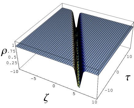
Figure 2: This displacement is similar to the well known ”classical bubble” solution in field theory, but for our case it represents the agglomeration of units in the molecular chain and for this reason it is named ”crowdon” ( 21)

This result is linked to solutions that are moving slowly with less velocity in comparison with the sound velocity, i.e. when $v_{s}^{2}-v^{2}>0$. But when the opposite occurs, i.e. when the soliton velocity is greater than the sound velocity we have soliton solution on the step or on the background. This type of solution is presented in the Fig. 3.

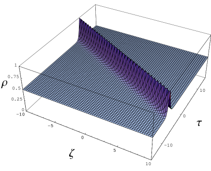
Figure 3: Typical soliton like perturbation on the background that represents the displacements. The interpretation that could be given to this solution is that in a real manner represents a bubble or the region inside of which the displacements are increasing and this effect is contrary to the agglomeration.

So, the sign of $G$ determines the type of soliton solution for the displacement that corresponds to the distribution of excitations. When $1<A<4,$ bubble solitons for the excitations appear corresponding to displacements of both types: popular gray solitons and normal ”bell” soliton on the background. In the first case for displacements we have obtained the crowdon solution. In the last case, this displacement shows a huge separation between neighborhoods in the molecular chain. This solution travels along the protein with velocity $v$ greater than the acoustic velocity. Of course, we have here a little difference of popular bubbles of other nonlinear equations. As it is well known, the classical bubble is characterized by the rarefaction inside crucial region, but in this case, the feature of our solution is contrary to this best known property of classical bubbles. Indeed, the displacements outside the perturbed region have constant values, while inside of this region the separation between molecules increase as shown in Fig. 3. When this displacement is strong enough, one could observe the breaking of the protein chain and the solution could be transformed to a peak or cusp like non-classical solution.

IV.2.2 Crowdon solutions

The ”space” of our model is a line with two points as boundaries at the infinite. The existence of topological soliton named kink, is due to the properties of the mapping between the degenerated minimums of the potential, with the space, saying better, with its boundaries, that in this case it is a discrete set.

Kink solitons appear when the potential supports degenerated absolute vacua in $\varphi=\kappa_{3}=\frac{2A+1}{3}$, when $A>4$. So, the boundary conditions for this case, are

$$\varphi\left(\zeta=-\infty\right)=-\kappa_{3},\;\varphi\left(\zeta=\infty\right)=\kappa_{3}.$$

The kink solution has the following form

$$\varphi_{k}=\frac{\sqrt{A-4}}{\sqrt{3}}\frac{e^{i\theta}\sinh[2\sqrt{a}(y-y_{0})]}{\sqrt{1+\frac{A-4}{2A+1}\cosh^{2}[2\sqrt{a}(y-y_{0})]}}.$$ (23)

For antinkink, as usual, we can take the inverse signs, so when $x\rightarrow+\infty\,$, the field will approach the value $-\kappa_{3},$. Calculating the topological charge of this solution we obtain $Q_{k}=1$. For the antikink, we have $Q_{ant}=-1$. In this case, the regular solutions with finite energy are divided in 4 topological sectors. The sectors with finite energy can be characterized by means of the following pairs of indices $(-\kappa_{3},\kappa_{3}),(\kappa_{3},-\kappa_{3}),(-\kappa_{3},-\kappa_{3})$ and $(\kappa_{3},\kappa_{3})$ that correspond to the values of the field at infinities i.e. for $\varphi\left(x=-\infty\right),\;\;\varphi\left(x=+\infty\right)$. The kink, antikink and trivial solutions $\varphi\left(x\right)=\pm\kappa_{3}$ are the members of the $4$ sectors.

Using the equations (23) and (10) For the displacement $\rho(\zeta,\tau)$ we have the following expression

$$\rho(\zeta,\tau)=\frac{m\beta D}{RM}\left(\frac{\sinh^{2}\left[2\sqrt{a}(y-y_{0})\right]}{\alpha_{3}+\alpha_{4}\cosh^{2}\left[2\sqrt{a}(y-y_{0})\right]}\right),$$ (24)

with

$$\alpha_{3}=\frac{3G}{A-4}+\kappa,\ \ \ \ \alpha_{4}=\frac{3G}{2A+1}-\kappa,$$

and $\kappa$ is defined in equation (22).

Considering positive values for $\alpha_{i}$ when the boundaries values of displacements are fixed, there is a possibility of emergence of crowdons that will propagate along the chain. The displacements show the typical picture of ”classical” bubble solitons. This bubble in the molecular chains context is not a dip in the background. On the contrary, this solutions represent the wave agglomeration of molecular units traveling along the chain. So, along the molecular chain the distribution of excitations evolves like a kink soliton while its corresponding displacement evolves like typical crowd like soliton solutions, see Fig. 4.

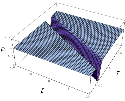
Figure 4: The evolution of the displacements shows typical characteristic of ”crowd” soliton solution. For a qualitative representation of the solution, we take the values $\alpha_{4}=1,\alpha_{3}=3,v=-1.2$. Apparently, this picture represents ”classical bubble” solitons but inside the perturbed region the displacements reduce their values forming the crowdons (24).

IV.3 Stability and Self-localizations

Next, we can use some results concerning the possibility of stabilizations of those types of solitons we have found in the section A and B for those distribution of excitations with non- topological charges. We will follow the findings of the paper bernal

As it is well known, our system is closely related to the phi-six theory, that shows several important behavior in nuclear hydrodynamics, ferromagnetism, phase transitions and other branches of physics and natural sciences makha . The equation of motion that we will analyze in the context of self localization is the equation (12) obtained above.

The main ideas of the approach developed in makha and bernal could be summarized as follows: This method in some sense is similar to Lyapunov functional approach for analyzing stability problems. For the general multidimensional case of spherical or cylindrical symmetry the dynamical system associated with the solitons NSE is:

$$i\psi_{t}+\psi_{rr}+\frac{\mathcal{D}-1}{r}\psi_{r}-\frac{dU(\Phi)}{d\Phi}\psi=0,$$ (25)

where $\Phi\equiv$ $\psi^{\ast}\psi$ , the dimension of the space is $\mathcal{D}$ and with suitable change of parameters we use the potential part of the energy as makha ; bernal

$$U\left(\Phi\right)=U(\Phi)=\Phi+2A\Phi-\left(2+A\right)\Phi^{2}+\Phi^{3},$$

with

$$A=-2-\frac{3}{4\alpha}(1+\sqrt{1+4\alpha}),$$

and $\alpha$ is defined by the equation (14). For our case, a molecular system, the equation (25) is the same equation (12) with $\mathcal{D}=1$ me . The constant solutions of the equation (11) at $A=-\frac{1}{2}$ undergoes a supercritical bifurcation.

For analyzing the self-localizations of soliton structures we will evaluate the behavior of the following functional $B(t)$ makha ; bernal

$$B(t)\equiv\pi 2^{\mathcal{D}-1}\int\Psi^{\ast}\Psi r^{D+1}dr=\langle r^{2}\rangle N\geq 0,$$ (26)

where $N$ denotes the ”number of particles” integral of motions. The magnitude $B(t)$ represents in some sense the width of the soliton solution obtained in this model. As it can be seen from the equation (26) the functional $B(t)$ is proportional to the expectation value of the square of the position. From here this magnitude is proportional to the width of the soliton solution. Let us evaluate the second derivative of this magnitude and we obtain

$$\frac{d^{2}B(t)}{dt^{2}} =$$ (27)

$$2^{\mathcal{D}-1}\pi\left\{8\int\left|\psi_{r}\right|^{2}dr+4\mathcal{D}\left[\int\left(\frac{dU}{d\Phi}\Phi-U\right)dr\right]\right\}.$$

As we are concerned with solitons in one dimensional case for the molecular system, finally making $\mathcal{D}=1,$ and evaluating the conditions under self-localization of soliton structures we finally obtain that following conditions bernal

$$\text{If }\,\mathcal{D}=1,\;\;\;\frac{\delta\ddot{B}}{\delta\mathfrak{V}}<0,\,\;\;\;\text{for \ \ \ }A<2,$$ (28)

where $\mathfrak{V}$ denotes the ”volume” of the soliton structure. Now let us calculate the possible values of the parameters for getting self localizations of solitons. We make $\alpha=-\varrho$ and for satisfying the condition (28) we obtain the inequality

$$\frac{1}{\varrho}\left(1+\sqrt{1-4\varrho}\right)<\frac{16}{3}$$ (29)

with $\varrho=\frac{\lambda\gamma}{2\beta D}.$ As we can see from the relation (29) for all values of $\varrho<0,$ the self-localization is possible i.e. when the parameters satisfy this relation $\frac{\lambda\gamma}{2\beta D}<0$. In the case of positive region of the axis $\varrho$, we can conjecture that self-localizations would occur when

$$0.2345\leq\frac{\lambda\gamma}{2\beta D}\leq 0.25$$

That means, we should try to find stable soliton like solutions within this sector that could determine the possible values of the relevant parameters in real experiments.

V Conclusions

We have taken into consideration in some sense an improved Davydov‘s model, and obtained a nonlinear evolution equation for the displacement that in mutual coordination with the excitation generate nontopological and topological solitons.

When the molecular system evolves, it is of course interesting to know which types of structures it could support during its evolution when its dynamic is modeled by the cubic quintic nonlinear Schrodinger equation. When the boundary condition is of the trivial one, we obtained a typical well known ”bell” soliton that represents the separation of the molecular units inside the perturbations. Let us make some comments about the physical meaning of the solution obtained when we considered the condensate type of boundary conditions. In this specific case, the molecular model subjected to both ”condensate boundary conditions”, in both directions, the displacements $\rho$ acquires a constant value. This means that due to multiple internal or external factors that affects the molecular system, the displacement far from the perturbed region acquires some certain values that in some sense could be considered as established during the process of the existence. In the case, when bubble like solutions appear as natural excitations, displacements around the central part of the perturbed region could be of two types: the first one corresponds to the crowd solutions, that means we have in some sense an agglomeration of units that compound the lattice i.e. a ”crowdon”. This agglomeration travels along the chain with velocity $v_{s}$ less than that of the sound. The second solution for displacements is the ”soliton on the step” and travels faster than sound. It represents the increasing of distance between elemental units inside the perturbed region of the molecular chain. For the case, when the excitations reveal the typical profile of kink solutions, as we can see from equations (24), the displacements apparently evolve like ”classical bubble” solitons but they represent the crowdons again, and represent the agglomeration of units along the molecular chain. According to the stability analysis, we also conjecture that it is possible to obtain stable solitons inside the narrow segment in the parametric domain determined by the equation (IV.3). Finally, it should be interesting to check in more realistic models, the behaviors of these structures after the inclusion of , for example, dissipation term to describe the effects from water molecules surrounding the molecular system.

- (1) A.C. Scott, Phys rep. 1 (1992) 217.
- (2) A.S. Davydov and N.I. Kislukha. Sov. Phys. JETP 44, n3 (1976) 571- 575
- (3) W. Han, S. M. Lindsay, M.Dlakic, and R.E. Harrington, Nature 563 (1997) 386.
- (4) W. Han, M. Dlakic, Y.-J. Zhu, S.M. Lindsay, and R.E. Harrington, Procc Natl.Acad. Sci. USA 94 (1997) 10565.
- (5) J. Agrawal, D. Hennig, Physica A 323 (2003) 519-533.
- (6) J. Cuevas, F. Palmero, JFR. Archilla and FR. Romero, Theor. Mat. Phys. 137 (2003) 1406-1411.
- (7) Pl. Christiansen, YB. Gaididei and SF. Minagleev, Jour. Phys. - Cond. Math. 13 (2001) 1181-1192.
- (8) M. Daniel and N. M. Latha, Physica A 298 (2001) 351-370.
- (9) A.C. Scott, Phys. Scripta 29 (1984) 279.
- (10) M. Toda, Phys. Rep. 81, 1 (1975)
- (11) V.G. Makhankov, Soliton Phenomenology, Kluwer Academic Publisher 1900
- (12) M. Agüero, Physics Letters A 278 (2001) 260.
- (13) V.G. Makhankov. Dynamics of classical solitons. Phys Reports 35 (1978) 1-128.
- (14) D.E. Pelinovsky, Yu. S. Kivshar and V.V. Afanasjev. Phys Rev 54 (1996) 2015.
- (15) M.Aguero, J.Bernal and A.Makhankov, Chaos, Soliton and Fractals 12 (2001) 113-123