LPT-ORSAY/08-19

Parametrisations of the $D\to K\ell\nu$ form factor
and the determination of $\hat{g}$

Sébastien Descotes-Genon and Alain Le Yaouanc
Laboratoire de Physique Théorique,
CNRS/Univ. Paris-Sud 11 (UMR 8627), 91405 Orsay Cedex, France

The vector form factor $f_{+}(t)$ of the semileptonic decay $D\to K\ell\nu$, measured recently with a high accuracy, can be used to determine the strong coupling constant $g_{D_{s}^{*}DK}$. The latter is related to the normalised coupling $\hat{g}$ releveant in heavy-meson chiral perturbation theory. This determination relies on the estimation of the residue of the form factor at the $D_{s}^{*}$ pole and thus on an extrapolation of the form factor in the unphysical region $(m_{D}-m_{K})^{2}<t<(m_{D}+m_{K})^{2}$. We test this extrapolation for several parametrisations of the form factors by determining the value of $\hat{g}$, whose value can be compared to other (experimental and theoretical) estimates. Several unsophisticated parametrisations, differing by the amount of physical information that they embed, are shown to pass this test. An apparently more elaborated parametrisation of form factors, the so-called $z$-expansion, is at variance with the other models, and we point out some significant shortcomings of this parametrisation for the problem under consideration.

The weak transitions from one meson to another provide very interesting tests of our understanding of the Standard Model both in the weak and strong sectors. On one hand, elements of the Cabibbo-Kobayashi-Maskawa matrix can be determined by comparing the experimentally measured decay rate with a theoretical value obtained at one or several kinematic points: for instance $B\to D\ell\nu$ for $|V_{cb}|$, $B\to\pi\ell\nu$ for $|V_{ub}|$, or $K\to\pi\ell\nu$ for $|V_{us}|$. On the other hand, the shape of the spectrum provides a stringent check of our description of the dynamics of hadrons governed by QCD.

The hadronic physics of the problem is encoded in form factors, which are complicated nonperturbative objects. Due to our limited theoretical knowledge of these objects, many parametrisations are available, trying to include as much information as possible on the (known or assumed) dynamics of the corresponding mesons. Recently, the BaBar collaboration has performed a very accurate analysis of the $D^{0}\to K^{-}e^{+}\nu_{e}$ decay [1] (see also the work done by the CLEO collaboration [2]). The relevant form factors are defined as

$$\langle K(p^{\prime})|\bar{s}\gamma_{\mu}c|D(p)\rangle=\left(p_{\mu}+p^{\prime}_{\mu}-q_{\mu}\frac{m_{D}^{2}-m_{K}^{2}}{q^{2}}\right)f_{+}(t)+q_{\mu}\frac{m_{D}^{2}-m_{K}^{2}}{q^{2}}f_{0}(t)$$ (1)

with $q=p-p^{\prime}$ and $t=q^{2}$. Ref. [1] determined very precisely the $t$-dependence of the vector form factor $f_{+}$ (the scalar form factor $f_{0}$ could not be obtained because of the very light mass of the electron). We can provide a general expression of this form factor in terms of an unsubtracted dispersion relation (such an unsubtracted dispersion relation is allowed by the asymptotic behaviour expected from QCD):

$$f_{+}(t)=\frac{{\rm Res}(f_{+})}{m_{D_{s}^{*}}^{2}-t}+\frac{1}{\pi}\int_{t_{+}}^{\infty}dt^{\prime}\frac{{\rm Im}\ f_{+}(t^{\prime})}{t^{\prime}-t}$$ (2)

where

$$t_{+}=(m_{D}+m_{K})^{2}\qquad t_{-}=(m_{D}-m_{K})^{2}$$ (3)

meaning that we have a pole at $m_{D_{s}^{*}}^{2}$ ($m_{D_{s}^{*}}=2.112$ GeV) and a cut from the $DK$ continuum . We have defined ${\rm Res}(f_{+})$ so that it be positive.

The physical region for the semileptonic decay is $0<t<t_{-}$, where high-precision experimental information is available [1]. Although it corresponds to an unphysical point between the semileptonic region and the $DK$ cut, the pole residue is physically interesting. Indeed it is related to the $D$-$K$-$D^{*}_{s}$ strong coupling (with a subsequent weak decay of $D^{*}_{s}$ into a lepton pair), which itself linked to $g_{D^{*}D\pi}$ by $SU(3)$ symmetry. This latter coupling is a fundamental ingredient for Heavy Meson Chiral Perturbation Theory [3, 4, 5, 6] and allows one to compute the effect of pion and kaon exchanges on the non-perturbative dynamics of heavy-light mesons (see refs. [7, 8, 9] for recent applications to semileptonic decays and other processes, as well as pending issues in this field).

We want to exploit the good experimental knowledge on $f_{+}$ in the physical region to determine the residue ${\rm Res}(f_{+})$ and thus $g_{D^{*}_{s}DK}$ by an extrapolation of the form factor from $t_{-}$ to $m_{D_{s}^{*}}^{2}$:

$$f_{+}(t)=\frac{f_{D_{s}^{*}}g_{D^{*}_{s}DK}/2m_{D_{s}^{*}}}{1-t/m_{D_{s}^{*}}^{2}}+\ldots$$ (4)

where $f_{D_{s}^{*}}$ is the decay constant relative to the purely leptonic decay of the $D_{s}^{*}$. $g_{D^{*}_{s}DK}$ is related to another significant quantity, the normalised matrix element of the axial current between the $B$ and $B^{*}$ mesons denoted $\hat{g}$.

For this extrapolation, we can devise analytical models or parametrisations describing the physical region as a function of $t$, and extrapolate the expression into the region near the pole. We then deduce the residue according to:

$${\rm Res}(f_{+})=\lim_{t\to m_{D_{s}^{*}}^{2}}(m_{D_{s}^{*}}^{2}-t)f_{+}(t)$$ (5)

It proves interesting to define a function ${\rm Res}(f_{+})(t)$, which we call the residue function, according to:

$${\rm Res}(f_{+})(t)=(m_{D_{s}^{*}}^{2}-t)f_{+}(t)\qquad\qquad{\rm Res}(f_{+})={\rm Res}(f_{+})(m_{D_{s}^{*}}^{2})$$ (6)

We can hope to get reasonable extrapolations by considering smooth representations of ${\rm Res}(f_{+})(t)$. Since we have factorised the pole denominator, the residue function has singularities only due to the cut.

Models will show differences in the way that they represent these singularities. We propose to use the value of $\hat{g}$ as a test to select the most appropriate models among the available ones. Indeed, we have independent experimental and theoretetical information on this coupling. Models with reasonable physical assumptions (i.e. the singularities along the cut) should be able to provide reasonable extrapolations from the semileptonic region to the $D_{s}^{*}$ pole, and thus to yield values of $\hat{g}$ in good agreement with our current knowledge.

Of course, the various heavy-to-light semileptonic decays could yield similar strong couplings, somewhat related by heavy quark or $SU(3)$ symmetries. To evaluate the specific interest of the reaction $D\to K\ell\nu$ in this respect, we can notice the following facts. Since

$$t_{-}/m_{D_{s}^{*}}^{2}=0.42\qquad t_{+}/m_{D_{s}^{*}}^{2}=1.24$$ (7)

the $D_{s}^{*}$ pole is relatively close to the threshold of the cut for $DK$ production, but far from the physical region for the semileptonic decay; in addition, the physical interval is not very large. This can be compared with other semileptonic heavy-to-light decays. $B,D\to\pi\ell\nu$, exhibit the advantage of a pole located very close to the physical region, and specifically for $B\to\pi\ell\nu$, the physical region is very extended. However the cut is now so close to the investigated pole that it may cause problems. For $B\to\pi l\nu$, the smallness of $|V_{ub}|$ makes an accurate measurement of the form factor near the $t=t_{-}$ endpoint very difficult: the decay rate is very small at this endpoint where its value is crucial for a good extrapolation.

$D\to\pi l\nu$ seems more promising in this respect, and it is complemented interestingly by $D\to K\ell\nu$. In the latter case, the pole lies farther than for $D\to\pi l\nu$, but it is better separated from the cut, and it is easier to observe because of the large value of the CKM matrix angle $V_{cs}$ (compared to the Cabibbo-suppressed $D\to\pi$ transition). On one hand this could be considered unfavourable: the extrapolation will remain undoubtedly uncertain, given the limited precision of the data, since many models may be very close in the physical region, but will greatly differ near the pole. On the other hand, it provides an interesting opportunity to test these parametrisations in a situation where their differences will be enhanced and thus easier to discuss.

This note is organised as follows. In Sec. 1, we discuss the essential ingredient of the dispersive representation of the form factor, namely the $DK$ cut. In Sec. 2, we introduce several parametrisations which differ mainly through their approximate description of the cut. In Sec. 3, we discuss the extrapolation of the form factor in the unphysical region according to these parametrisations. In Sec. 4, we collect the resulting values for the hadronic coupling constants $g_{D_{s}^{*}DK}$ and $\hat{g}$ and comment on the discrepancies induced by the different parametrisations, before drawing a few conclusions in Sec. 5.

1 The $DK$ cut

Theoretical inputs concerning the cut associated with $DK$ production are essential since it governs the behaviour of the residue function ${\rm Res}(f_{+})$. There are none compelling. Yet we can consider two partial and complementary contributions from the low-energy $DK$ continuum and from resonances.

First, consider the contribution to the cut stemming from the $DK$ low-energy continuum. In the elastic regime, between the $DK$ threshold and the first inelastic threshold, one has

$${\rm Im}f_{+}(t)=\sqrt{\lambda}{t}f_{1}^{DK}(t)f_{+}(t)\theta(t-(M_{D}+M_{K})^{2})$$ (8)

where $\lambda=(t-t_{+})(t-t_{-})=4tq^{2}$ and $f_{1}^{DK}$ is the $P$-wave amplitude for $DK\to DK$ scattering. Close to the $DK$ threshold (small positive $q^{2}$), the form factor has the following behaviour in $q^{2}$

$$f_{1}^{DK}(t)\sim A_{1}q^{2}$$ (9)

so that

$${\rm Im\ }f_{+}^{DK}(t)\sim A_{1}q^{3}$$ (10)

which means that the imaginary part departs slowly from zero above the $DK$ threshold: the cut should be very smooth.

Secondly, there are resonances all along the cut, corresponding to the successive radial excitations of the $D_{s}^{*}$, the first of which should be close to the $DK$ threshold. Indeed, with an excitation energy of order $0.5$ GeV added to the $D_{s}^{*}$ mass , we get a first radial excitation around $2.6$ GeV, while the cut starts at $m_{D}+m_{K}\simeq 2.4$ GeV. If we worked in the large-$N_{c}$ approximation of resonances with vanishing widths, the cut of the form factor $f_{+}$ would be largely dominated by the pole of the first excitation. On the other hand, in the actual world, most of the resonances acquire a broad width through their strong decays, will overlap and interfere, yielding a rather smooth cut. This is presumably true even for the lowest radial excitation, if the coupling constant is not exceptionally small, because of the allowed phase space, so that the impact of this first resonance on the cut is presumably mild. These arguments are supported by the recent observation of the $D_{sJ}(2700)^{+}$ by the Belle collaboration [11]. This meson is interpreted as a radially excited $c\bar{s}$ state with $J^{P}=1^{-}$ with a mass $M=2708\pm 9^{+11}_{-10}$ MeV, quite far away from the start of the cut, and a fairly broad width $\Gamma=108\pm 23^{+36}_{31}$ MeV.

Even though we have arguments supporting the smooth rise of the cut above threshold, it would be useful to estimate the absolute strength of the cut in order to constrain our extrapolation more tightly. Ideally, a determination of the vacuum-to-$DK$ matrix element would provide the basis for an interpolation between the physical region for the semileptonic and the region of the cut, rather than an extrapolation. Since this piece of information is currently lacking, we have to rely on parametrisations of the form factor.

2 Parametrisations of the form factor

We speak of “parametrisations” because we have admittedly little theory behind them. They are functions of $t$ with the following main merits: 1) in the physical region they collect the data of the form factors in a both simple and accurate description; 2) they incorporate in a rough way the few safe statements that we can formulate about the form factors outside the physical region, so that they may still be trusted at least at a certain distance from the physical region (of course, it remains an assumption that we can trust them as far as the pole). As summarised in eq. (2), we know that there is a pole at the known value $t=m_{D_{s}^{*}}^{2}$, and a cut begins at $t=(m_{D_{s}^{*}}+m_{K})^{2}$. The various parametrisations propose explicitly or implicitly different simplifications in the treatment of the cut, and we will sketch the salient features of the most widely used ones.

In the case at hand, $D\to K\ell\nu$, the experimental data is so accurate that the best option consists in fitting the parameters of the parametrisations on the data in the physical region. It turns out that most of them fit the data equally well in the semileptonic region. A particular representation would exhibit a decisive advantage if it were able to describe the unphysical region between the semileptonic region and the cut with the same parameters.

2.1 $z$-expansion

A parametrisation which is by now rather popular, yet apparently sophisticated, is the $z$-expansion [12, 13], which dates back to Boyd et al. (see ref. [14] and the works with Grinstein and Lebed quoted therein) where it was applied to heavy-to-heavy transitions. In principle, it has been devised to offer a good representation of form factors and we recall some steps of its derivation below.

One aims at writing down $f_{+}$ as a series $\Sigma~{}a_{i}z(t)^{i}$. The expansion parameter $z(t)$ is defined as:

$$z(t,t_{0})=\frac{\sqrt{t_{+}-t}-\sqrt{t_{+}-t_{0}}}{\sqrt{t_{+}-t}+\sqrt{t_{+}-t_{0}}}\propto t_{0}-t$$ (11)

with a free parameter $t_{0}$. $z(t)$ remains small over the whole physical region, and maps the complex $t$-plane into a disk of radius 1, with the cut in $t$ being transformed into the circle $|z|=1$. Ref. [12] advocates the choice $t_{0}/t_{+}=1-\sqrt{1-t_{-}/t_{+}}$ ($t_{0}/m_{D_{s}^{*}}^{2}=0.23$), which implies that $z(t)=0$ occurs for $t$ in the middle of the physical region [$z(0)=0.0515$ and $z(t_{-})=-0.0515$]. The change of variables from $t$ to $z$ has often been used in the hope of getting a quicker convergence of the resulting series in the physical region.

It has been proposed to combine this idea with analyticity constraints in order to constrain further the coefficients of the $z$-expansion [12, 13, 14]. The starting point is the correlator

$$\Pi^{\mu\nu}(q)=i\int d^{4}x\ e^{iqx}\langle 0|T(\bar{s}\gamma^{\mu}c)(x)\ (\bar{s}\gamma^{\nu}c)^{\dagger}(0)|0\rangle=(q^{\mu}q^{\nu}-q^{2}g^{\mu\nu})\Pi^{T}(q^{2})+g^{\mu\nu}\Pi^{L}(q^{2})$$ (12)

which defines two polarisation functions (transverse and longitudinal). First, these functions can be bounded approximately at large momenta using the Operator Product Expansion. Second, these functions can be expressed in terms of their imaginary part through a dispersion relation. Using unitarity, one can express this imaginary part as a sum of various (positive) contributions, corresponding to the squared modulus of matrix elements $\langle H|\bar{s}\gamma^{\mu}c|0\rangle$, where $H$ denotes any arbitrary single- or multiple-particle state with the appropriate quantum numbers (each contribution contains a a factor coming from the phase space). It means in particular that the imaginary part is larger than the sole contribution from $H=DK$, i.e. from $f_{+}$, multiplied by a phase-space factor.

By choosing multiplying the series in $z$ by a carefully chosen factor denoted $\Phi$, one can convert the bound induced on $f_{+}$ by unitarity and OPE into a bound on the coefficients of the series in $z$. The $z$-representation can be written as follows:

$$z{\rm{-exp}}:\frac{f_{+}(t)}{f_{+}(0)}=\frac{P(0)\Phi(0,t_{0})}{P(t)\Phi(t,t_{0})}\times\frac{1+\frac{a_{1}}{a_{0}}z(t,t_{0})+\frac{a_{2}}{a_{0}}z^{2}(t,t_{0})}{1+\frac{a_{1}}{a_{0}}z(0,t_{0})+\frac{a_{2}}{a_{0}}z^{2}(0,t_{0})}$$ (13)

where

$$\Phi(t,t_{0})=N(t_{+}-t)(\sqrt{t_{+}-t}+\sqrt{t_{+}})^{-5}(\sqrt{t_{+}-t}+\sqrt{t_{+}-t_{0}})(\sqrt{t_{+}-t}+\sqrt{t_{+}-t_{-}})^{3/2}$$ (14)

where $N$ is a numerical normalisation factor. It is unimportant here, since we consider only ratios of the form factor to its value at $q^{2}=0$. The factor $P(t)=z(t,m_{D_{s}^{*}}^{2})$ includes the $D_{s}^{*}$ pole. As explained above, the coefficients $a_{n}$ are bounded by unitarity: $\sum~{}|a_{i}|^{2}<1$ with a properly chosen normalisation constant $N$ [12, 13, 14].

In heavy-to-light processes, this expansion seems less useful, because it appears that all the coefficients $a_{n}$ that can be determined are anyway much smaller than the unitarity bound in absolute value [1], and nothing safe can be said about the relative magnitude of the coefficients with respect to the first one (see the fits in sec. 3). There remains a useful bound on the rest of the series, obtained by using Cauchy’s inequality:

$$\left|\sum_{n}^{\infty}a_{i}z^{i}\right|\leq\sqrt{\sum_{n}^{\infty}|a_{i}|^{2}}\sqrt{\sum_{n}^{\infty}|z^{i}|^{2}}\leq\sqrt{\frac{|z|^{2n}}{1-|z|^{2}}}$$ (15)

This bound, given the observed values of the form factor, is sufficiently small to be meaningful: it shows that the necessary number of terms should be about 2 or 3 to get a one percent accuracy in the semileptonic region. Actually, it was found that 2 or 3 terms are sufficient to fit the data [1], the last coefficient ($a_{2}$) being already affected by a large uncertainty. Unfortunately, this accurate representation in the semileptonic region does not warrant an accurate extrapolation. Indeed, in the region $t_{-}<t<t_{+}$, $z(t$) by no means remains small in this region $t_{-}<t<t_{+}$, since at the pole, $z(m_{D_{s}^{*}}^{2})=-0.340$ and at the beginning of the cut, $z(t_{+})=-1$. In this region, the bound eq. (15) becomes ineffective, or indicates that very many terms could be necessary.

2.2 Alternative representations

This parametrisation can be compared with other less sophisticated parametrisations

$${\rm Pole}:\frac{f_{+}(t)}{f_{+}(0)} = \frac{1}{\left[1-\frac{t}{m_{pole}^{2}}\right]}$$ (16)

$${\rm BK}:\frac{f_{+}(t)}{f_{+}(0)} = \frac{1}{\left[1-\frac{t}{m_{D_{s}^{*}}^{2}}\right]\left[1-\alpha\cdot\frac{t}{m_{D_{s}^{*}}^{2}}\right]}$$ (17)

$${\rm Linear}:\frac{f_{+}(t)}{f_{+}(0)} = \frac{1}{1-\frac{t}{m_{D_{s}^{*}}^{2}}}\left[1+c_{1}\cdot\frac{t}{m_{D_{s}^{*}}^{2}}\right]$$ (18)

$${\rm Quadratic}:\frac{f_{+}(t)}{f_{+}(0)} = \frac{1}{1-\frac{t}{m_{D_{s}^{*}}^{2}}}\left[1+c_{1}\cdot\frac{t}{m_{D_{s}^{*}}^{2}}+c_{2}\cdot\frac{t^{2}}{m_{D_{s}^{*}}^{4}}\right]$$ (19)

• The pole parametrisation is certainly too naive, since there is no reason for the lowest lying pole to saturate the form factor. Not surprisingly, one finds the pole much below its actual position (the $D_{s}^{*}$ mass). We will not use this parametrisation to perform an extrapolation of $f_{+}$ to the $D_{s}^{*}$ mass; it serves only to show that the achieved experimental accuracy requires to go beyond the common assumption of the dominance by the lowest pole in the physical region.

• The BK parametrisation [15] is well known in the analysis of $B$-decays, and it is mainly motived by the scaling laws of the form factors in the heavy quark limit. For a $D$ decay, this motivation is certainly weaker, but it is useful by providing a crude representation of the cut by an additional pole, with a free mass which comes out neatly above the start of the cut, at $t=m_{D_{s}^{*}}/\alpha$, with $\alpha$ smaller than $1$ to be consistent with the location of the cut. Let us stress that this second pole is not to be identified with any particular resonance. This effective pole sums up the effect of infinitely many resonances with positive or negative contribution (note that the additional BK pole has a contribution opposite in sign to $D_{s}^{*}$).

• Almost equivalent in practice, the ”linear” and ”quadratic” parametrisations follow old ideas from current algebra. They assume that the amplitude have a polynomial dependence of low degree in the momenta, once the lowest lying (ground state) poles have been factored out. Such an expansion is justified in the case of a weak cut, which can be approximated by its expansion in $t$ with a reasonable accuracy.

• Another parametrisation can be obtained by considering the $z$-expansion and replacing $\Phi$ with a constant. Obviously, no unitarity bounds can be derived in such a case: we have just performed a change of variable (reexpressing a $t$-series into a $z$-series) and extracted the $D_{s}^{*}$ pole. In order to distinguish these two versions of the $z$-expansion method, we call “simple $z$-expansion” the parametrisation with $\Phi(t)$ set to 1, and “unitary $z$-expansion” the expansion relying on eq. (14), which allows to exploit unitarity constraints (at least in principle) and described for instance in refs. [12, 13, 14].

3 Fit of the parametrisations to $D\to K\ell\nu$ data

Before extrapolating these various parametrisation to the $D_{s}^{*}$ pole, we need to determine their parameters from the data in the physical region. A fit of $z$-expansion, BK and pole parametrisations has been made in ref. [1] with data corrected for radiative effects. Unfortunately, the data (values of the form factors and correlation matrix) provided in this reference are only given before the correction of radiative effects. According to ref. [1], the main correction corresponds to an increase of the value of the first bin. Therefore, for each parametrisation we can compare three different fits depending on the set of data:

• The data before radiative corrections and the correlation matrix before radiative corrections (performed by us),

• The data with the first bin increased and the correlation matrix before radiative corrections (performed by us),

• The data and the correlation matrix with full radiative corrections (performed in ref. [1] and by us).

Model	Model param	No radiative corr	First bin corrected	Full radiative corr
Unitary $z$-exp	$a_{1}/a_{0}$	$-2.43\pm 0.25$	$-2.43\pm 0.25$	$-2.5\pm 0.28$
	$a_{2}/a_{0}$	$-4.26\pm 6.67$	$-2.98\pm 6.67$	$0.6\pm 7.8$
	correl	-0.82	-0.82	-0.86
BK	$\alpha$	$0.38\pm 0.03$	$0.37\pm 0.04$	$0.377\pm 0.037$
Pole	$m_{pole}$	$1.89\pm 0.02$	$1.89\pm 0.02$	$1.884\pm 0.019$
Linear	$c_{1}$	$0.43\pm 0.04$	$0.43\pm 0.05$	$0.42\pm 0.05$
Quadratic	$c_{1}$	$0.45\pm 0.15$	$0.41\pm 0.15$	$0.33\pm 0.15$
	$c_{2}$	$-0.036\pm 0.42$	$0.046\pm 0.42$	$0.25\pm 0.42$
	correl	-0.96	-0.96	-0.96
Simple $z$-exp	$a_{1}/a_{0}$	$-4.27\pm 0.26$	$-4.28\pm 0.26$	$-4.34\pm 0.26$
	$a_{2}/a_{0}$	$3.13\pm 6.73$	$4.41\pm 6.74$	$7.78\pm 6.79$
	correl	-0.85	-0.85	-0.85

Table 1: Parameters of the different parametrisations of $f_{+}$ from a fit to $D\to K\ell\nu$ data, with various treatments of radiative corrections (not included, partially included, fully included).

The parameters of the different models are collected in Table 1. Apart from the pole model, which does not fit the data very well, the other models yield very similar fits. The corresponding minimal values of the $\chi^{2}$ remains between 7 and 8, for 7 or 8 degrees of freedom (fit with 2 or 1 parameter).

The first three entries of the last column are taken from ref. [1, 16], where we combined systematic and statistic uncertainties in quadrature. Unfortunately, the three other parametrisations (linear, quadratic and simple $z$-expansion) have not been considered in [1]. As a poor man’s way of getting some information on the impact of radiative corrections for these two parametrisations, we have performed a fit with:

• The correlation matrix provided in ref. [1]

• The central values in each bin obtained from the $z$-parametrisation, using the values of $a_{1}/a_{0}$ and $a_{2}/a_{0}$ obtained including the radiative corrections.

We have checked that this procedure leads to values and uncertainties for the fitted parameters of the different models which are very similar to those quoted in ref. [1]. However, this procedure is admittedly a very imperfect attempt of getting a handle on radiative corrections, and should be replaced by a full treatment of radiative corrections for these three parametrisations, which can be done only by our experimental colleagues.

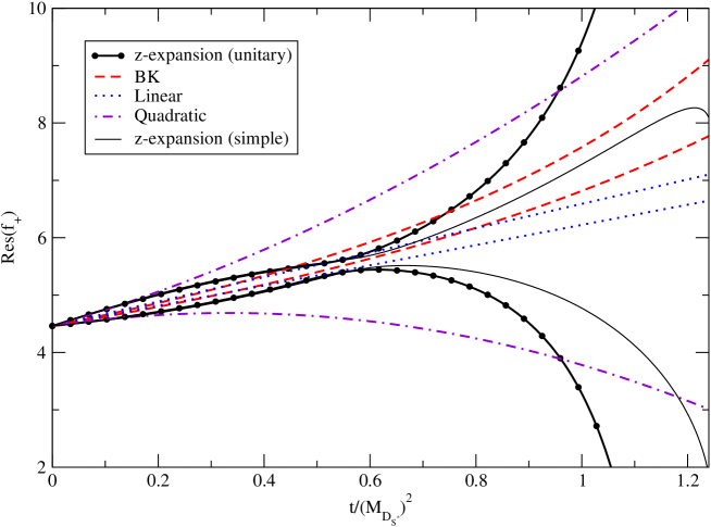
Figure 1: Range of variation for the function ${\rm Res\ }f_{+}(t)=f_{+}(t)(m_{D_{s}^{*}}^{2}-t)$ related to the residue of the form factor at the $D_{s}^{*}$ pole as a function of $t/M_{D_{s}^{*}}^{2}$, for the different parametrisations considered. No radiative corrections are included.

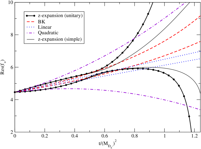
Figure 2: Range of variation of the function ${\rm Res\ }f_{+}(t)=f_{+}(t)(m_{D_{s}^{*}}^{2}-t)$ related to the residue of the form factor at the $D_{s}^{*}$ pole, as a function of $t/M_{D_{s}^{*}}^{2}$, for the different parametrisations considered. The effect of radiative corrections is included according to ref. [1] in the case of unitary $z$-expansion and BK models (see the text for the treatment of radiative corrections for the other models).

Figs. 1 and 2 illustrate the range of variation allowed for the residue function according to the different parametrisations, respectively before and after radiative corrections are taken into account. A striking difference can be observed between the (unitary) $z$ representation and the other parametrisations, the errors in the first case exploding beyond $t/m_{D_{s}^{*}}^{2}\simeq 0.8$. This behaviour can be understood from the explicit expression of the $z$-expansion. One must note the important factor $t_{+}-t$ in the definition of $\Phi(t,t_{0})$, eq. (14). This factor implies that the $z$-expansion includes a spurious, unwanted pole at the threshold of the cut, a feature which is very disadvantageous when the expansion is used not far from the cut, as needed to make our extrapolation. To be used there, the $z$-expansion requires in principle a very large number of terms in the series $\Sigma~{}a_{n}z^{n}$, and of course so many $a$’s cannot be determined from the knowledge of the physical region. At most, the first two or three coefficients can be estimated, so that the spurious threshold pole has a very strong effect on extrapolation. At the start of the cut, the $z$-expansion becomes meaningless.

The complicated form of $\Phi$ was chosen to translate the unitarity conditions on $f_{+}$ into a constraint on the coefficients $a_{n}$ of the $z$-expansion. In particular, the troublesome threshold pole is related to the two-body phase space arising in the unitarity bound on $f_{+}$. On the other hand, it turns out that the bound on the coefficients $a_{n}$ is far from saturated, and thus of little impact on the problem at hand, so that it can be left out without consequence, as exemplified by the “simple” $z$-expansion (with $\Phi=1$).

It is also interesting to compare this parametrisation with the BK parametrisation. Both representations have a pole in addition to $D_{s}^{*}$, but the former fixes it at threshold while the latter keeps this pole at $t=m_{D_{s}^{*}}/\alpha$ as a free parameter. This effective pole sums up the contributions of a tower of resonances to the cut. We find that $\alpha<1$, consistently with the location of the cut. Let us also recall that one should have $\alpha\to 1$ in the heavy-quark limit and large-energy release limit: therefore, it is consistent to get something rather different from $1$ in the decay $D\to K\ell\nu$ .

4 The strong coupling $g_{D_{s}^{*}DK}$

Extrapolating the results of the previous section to the $D_{s}^{*}$ pole and propagating the errors, we obtain $g_{D^{*}_{s}DK}$ through eq. (4), which is related to the matrix element of the axial current between the $B$ and $B^{*}$ mesons. After a suitable normalisation of states, this matrix element is denoted as $\hat{g}$ and one has :

$$\hat{g}=\frac{f_{K}g_{D^{*}_{s}DK}}{\sqrt{m_{D}m_{D_{s}^{*}}}}$$ (20)

$\hat{g}$ is finite in the heavy-quark mass limit, and thus should vary slowly with the heavy-quark mass. Another important property is that the strong couplings of the $K$ meson (Goldstone boson) with the $D$ and any other $D_{s}$-type state satisfy an Adler-Weisberger sum rule, with all the intermediate states contributing positively, yielding a bound on the $g_{D_{s}^{*}DK}$ coupling. In terms of $\hat{g}$, this bound is quite simple:

$$|\hat{g}|<1$$ (21)

The upper bound cannot be reached because there are indeed transitions from the $D$ meson to other states than the $D_{s}^{*}$. The limit $1$ corresponds to a completely non-relativistic calculation (for more details on $\hat{g}$, see for instance ref. [10]).

Numerically, we take $f_{K}=154$ MeV, $m_{D}=1.864$ GeV, $m_{D_{s}^{*}}=2.112$ GeV. Since $f_{D_{s}^{*}}$ has not been measured directly, we must rely on lattice calculations. $N_{F}=0$ calculations from the Rome [20] and UKQCD [21] lattice collaborations are available, with sizably different numbers. Unfortunately, neither papers quote their value of $f_{D_{s}^{*}}$ explicitly. In the case of the Rome collaboration, we have to pass through the ratio $f_{D_{s}^{*}}/f_{D^{*}}=1.10$ and the value of $f_{D^{*}}=258(14)(6)$ MeV. In the case of UKQCD, we have to convert their result from their dimensionless definition of $f_{D_{s}^{*}}=8.3$ to our definition $f_{D_{s}^{*}}=m_{D_{s}^{*}}/f_{D_{s}^{*}}^{UKQCD}$. In addition, it must be noticed that the mass $m_{D_{s}^{*}}$ must be taken consistently from the lattice data at the same $\beta$ and with the same way of fixing the lattice unit as $f_{D^{*}}$. We choose $\beta=6.2$ and we use $f_{\pi}$ to fix the lattice unit (as done to compute $f_{D_{s}^{*}}$) so that $m_{D_{s}^{*}}=2.061$ GeV. Following this procedure, we obtain finally the central values $f_{D_{s}^{*}}=284$ MeV (Rome) and $f_{D_{s}^{*}}\simeq 248$ MeV (UKQCD).

A very naive average yields the value $f_{D_{s}^{*}}=270$ MeV that we use in the following. We do not quote errors on the auxiliary quantity $f_{D_{s}^{*}}$: it would represent a very involved task for a quantity that we use only as a reference scale to compare different parametrisations. However, one should keep in mind that the value of this decay constant may be underestimated in view of the situation for the closely related quantity $f_{D_{s}}$. Indeed the same lattice groups predicted the latter around $230$ MeV, while the most recent experimental average [22] yields $275\pm 10$ MeV . If $f_{D_{s}^{*}}$ were to be enhanced, $g_{D^{*}_{s}DK}$ and $\hat{g}$ should be accordingly rescaled (and lowered). However, the hierarchy observed in the results of the extrapolations will not be affected by this change in the overall normalisation.

We have discarded the simple pole model in the discussion of the residue: it does not account for the data properly, even with a flexible vector meson mass, and it would be meaningless to discuss the residue with a fictitious pole mass.

Model	No radiative corr	First bin corrected	Full radiative corr
Unitary $z$-exp	$16.2\pm 7.8$	$17.9\pm 7.8$	$23.0\pm 8.7$
BK	$18.3\pm 1.1$	$18.2\pm 1.0$	$18.2\pm 1.2$
Linear	$16.3\pm 0.6$	$16.2\pm 0.6$	$16.1\pm 0.6$
Quadratic	$16.1\pm 6.5$	$16.6\pm 6.4$	$18.1\pm 6.4$
Simple $z$-exp	$15.4\pm 3.2$	$16.1\pm 3.2$	$18.2\pm 3.1$

Table 2: Values of $g_{D^{*}_{s}DK}$ obtained from different parametrisations of $f_{+}$, with various treatments of radiative corrections (not included, partially included, fully included).

Model	No radiative corr	First bin corrected	Full radiative corr
Unitary $z$-exp	$0.63\pm 0.31$	$0.70\pm 0.30$	$0.89\pm 0.34$
BK	$0.71\pm 0.04$	$0.70\pm 0.04$	$0.71\pm 0.05$
Linear	$0.64\pm 0.03$	$0.63\pm 0.03$	$0.62\pm 0.03$
Quadratic	$0.62\pm 0.25$	$0.64\pm 0.25$	$0.70\pm 0.25$
Simple $z$-exp	$0.59\pm 0.12$	$0.62\pm 0.13$	$0.71\pm 0.13$

Table 3: Values of $\hat{g}$ obtained from different parametrisations of $f_{+}$, with various treatments of radiative corrections (not included, partially included, fully included).

The results for $g_{D^{*}_{s}DK}$ and $\hat{g}$ are collected in Tables 2 and 3. Models describing the singularities of the cut in an appropriate way should yield values of $\hat{g}$ in good agreement with what has been obtained from experimental measurement of strong decays or from the lattice calculations.

The only indication from experiment is indirect because it concerns the $SU(3)$ counterpart of $g_{D^{*}_{s}DK}$, $g_{D^{*}D\pi}$. Indeed, CLEO [23, 24] has measured the decay width of $D^{*}\to D\pi$, from which they estimate:

$$g_{D^{*}D\pi}=17.9\pm 0.3\pm 1.9$$ (22)

leading to:

$$\hat{g}=0.59\pm 0.07\simeq 0.6$$ (23)

The latter value should apply roughly for the $D^{*}_{s}-D$ transition through $SU(3)$ flavour symmetry (the Dirac quark model and the lattice results suggest an increase when one increases the light quark mass up to the strange mass).

Model approaches can be used to determine this coupling. The Dirac model, see for example ref. [10], led to a result close to $\hat{g}\simeq 0.6$ for a static $c$ quark, a number close to what was found later in the above experiment. The application of a dispersive approach to a constituant quark model led to $\hat{g}$ from 0.4 to 0.5 [28, 18].

The result of lattice QCD simulations for the $D^{*}-D$ transition is, by extrapolation to the $u,d$ mass (ref. [29]):

$$\hat{g}=0.67(8)^{+4}_{-6}$$ (24)

which is compatible with the experimental number quoted above. The lattice can in fact measure directly another $SU(3)$ partner of the $D^{*}_{s}-D$ axial transition matrix element (corresponding to the $A_{1}$ form factor, up to a mass factor very close to $1$), i.e. $D^{*}_{s}-D_{s}$, since the lattice direct measurement is close to the strange quark mass; the result is close to $0.7$ from same reference, at $\beta=6.2$.

Comparing these values (all in the same range) with the above tables, which collect the coupling obtained by extrapolation of $D\to K\ell\nu$, we can make the following comments:

• The result from the (unitary) $z$-expansion is sensitive to the extraction of the radiative corrections on the whole range of momenta. With a full treatment of radiative corrections, one obtains a neatly larger number than with the other parametrisations, and the central value of $\hat{g}$ is close to the upper bound set by the Adler-Weisberger sum rule. We interpret this as a consequence of the spurious pole at $t=t_{+}$: this representation must be discarded when the unphysical region is concerned because of its unphysical behaviour at the threshold of the cut.

• The four other results are rather close to each other which is encouraging, since they rely on varied but reasonable assumptions on the smoothness of the cut. In particular, the simple $z$-expansion yields a value in good agreement with the other models, confirming that the spurious pole in $\Phi$, imposed by unitarity constraints, is the actual source of difficulties for the unitary $z$-expansion.

• For these four models, the central value is in agreement with the independent determinations of $\hat{g}$, in particular the experimental one. This provides further support for our preferred assumptions and parametrisations.

• One can check a posteriori that the effect of the cut is varying very slowly with $t$. Let us take the linear parametrisation as an illustration. After subtracting the pole which is at its right position and strength, the remaining contribution to the form factor is just a constant, that is, the cut is represented by a constant $c$, with $c_{1}=-0.42f_{+}(0)$ (the negative sign indicates that it has a lowering effect on the form factor). With such a parametrisation, we are sensitive to the structure of the cut neither in the physical region - which is perhaps not too surprising - nor in a large part of the unphysical region $t_{-}<t<t_{+}$.

• Comparing the ”quadratic” and ”linear” fits, we observe that a two-parameter fit, which seems equally reasonable as a one-parameter parametrisation, yields no change in the central value of $\hat{g}$; however, the errors are increased leading to a loss of predictive power. This means that the parametrisations are not constrained enough by the data in the physical region for a compelling extrapolation.

5 Conclusions

We have exploited recent high-precision data of the BaBar collaboration on the $D\to K\ell\nu$ decay in order to test various parametrisations of heavy-to-light form factors. Indeed, the current theoretical description of such form factors remains largely incomplete, and it can be improved by a direct comparison with data. The accuracy of the experimental results yields good fits of these parametrisations of the vector form factor $f_{+}$ in the physical region. But the value of the vector form factor outside this region is also of interest, since its residue at the mass of the $D_{s}^{*}$ meson is related to the strong coupling constant $\hat{g}$. To extract this quantity, we need to extrapolate the form factors outside the semileptonic region, and thus to rely on the properties and assumptions of the various parametrisations for $f_{+}$. On the other hand, the determination of $hat{g}$ and its comparison with values from other approaches (measurements of strong decays, lattice computations) provides an interesting test of the parametrisations of the form factors, since it probes the differences in the way these parametrisations representation the physical singularities along the cut.

In spite of the modesty of our approach, which is very phenomenological, some useful conclusions can be drawn:

• The method of extrapolation using smooth models for the cut - either a remote effective pole (BK) or a low-order polynomial in $t$ - has an encouraging success, since the $D_{s}^{*}$ residue appears quite compatible with values expected from very different considerations. The $z$ expansion (in its unitary version, widely popular by now) is disfavored: it contains a spurious pole at the threshold of the $DK$ cut which makes the extrapolation blow out of control in the unphysical region.

• The uncertainty on $f_{D_{s}^{*}}$ is still large; reducing it would in turn reduce that of the strong coupling constant and help to strengthen the previous conclusion.

• The extrapolation has by itself a very large uncertainty, which cannot be reduced further if we know only the physical region. Some quantitative theoretical knowledge about the form factor on the cut , in particular at threshold (scattering length…), would be a great help by transforming the extrapolation into an interpolation. Borrowing ideas from ref. [30], one could then use a sufficiently subtracted Omnès-Muskhelishvili representation to combine our knowledge on the cut near $DK$ threshold and the physical semileptonic region.

• Another improvement would consist in enlarging the interval of the fit. Such information could be provided by lattice simulations computing the form factor for $t<0$ (indeed they can calculate the $D-K$ matrix element without referring to the $D\to K\ell\nu$ transition). However, the improvement would be much milder, since the sensitivity to the cut decreases when one gets deeper into the region of negative $t$.

The $D\to K\ell\nu$ process is a particular decay among many similar semileptonic processes. It presents the advantage of a highly accurate knowledge of the form factor, and of a clear analytical structure, with the physical threshold, the pole and the cut neatly separated, which will not be the case for other processes. Our simple analysis of this particular process shows some interesting features of the different parametrisations of the form factors currently used to analyse weak transitions from one meson to another. In particular, it should invite practitioners to proceed with care when they have to rely heavily on parametrisations to extract quantities of physical interest (such as CKM matrix elements or strong hadronic couplings) with a high accuracy.

Acknowledgments

We thank Patrick Roudeau (LAL) who suggested and initiated this study, and who provided us many precious indications on the BaBar measurements of the form factor, as well as Damir Bećirević (LPT) for his numerous comments and discussions. Our work has also benefited from the various joint discussions between LAL experimentalists and LPT theorists.

This work was supported in part by the EU Contract No. MRTN-CT-2006-035482, “FLAVIAnet” and by the ANR project QCDNEXT (ANR_NT05-3_43577).

References

- [1] BABAR Collaboration, B. Aubert et. al., Measurement of the hadronic form factor in decays, Phys. Rev. D776 (2007) 052005, [0704.0020].
- [2] CLEO Collaboration, and others, A Study of the Semileptonic Charm Decays and , 0712.1020.
- [3] M. B. Wise, Chiral perturbation theory for hadrons containing a heavy quark, Phys. Rev. D45 (1992) 2188–2191.
- [4] T.-M. Yan et. al., Heavy quark symmetry and chiral dynamics, Phys. Rev. D46 (1992) 1148–1164.
- [5] G. Burdman and J. F. Donoghue, Union of chiral and heavy quark symmetries, Phys. Lett. B280 (1992) 287–291.
- [6] R. Casalbuoni et. al., Phenomenology of heavy meson chiral Lagrangians, Phys. Rept. 281 (1997) 145–238, [hep-ph/9605342].
- [7] S. Fajfer and J. F. Kamenik, Charm meson resonances in decays, Phys. Rev. D71 (2005) 014020, [hep-ph/0412140].
- [8] D. Becirevic, S. Fajfer, and J. F. Kamenik, Chiral behavior of the - mixing amplitude in the standard model and beyond, JHEP 06 (2007) 003, [hep-ph/0612224].
- [9] D. Becirevic, S. Fajfer, and J. F. Kamenik, Use and misuse of ChPT in the heavy-light systems, PoS LAT2007 (2007) 063, [0710.3496].
- [10] D. Becirevic and A. Le Yaouanc, coupling (): A quark model with Dirac equation, JHEP 03 (1999) 021, [hep-ph/9901431].
- [11] Belle Collaboration, J. Brodzicka et. al., Observation of a new meson in decays, Phys. Rev. Lett. 100 (2008) 092001, [arXiv:0707.3491].
- [12] R. J. Hill, The modern description of semileptonic meson form factors, hep-ph/0606023.
- [13] R. J. Hill, Constraints on the form factors for and implications for , Phys. Rev. D74 (2006) 096006, [hep-ph/0607108].
- [14] C. G. Boyd and M. J. Savage, Analyticity, shapes of semileptonic form factors, and , Phys. Rev. D56 (1997) 303–311, [hep-ph/9702300].
- [15] D. Becirevic and A. B. Kaidalov, Comment on the heavy to light form factors, Phys. Lett. B478 (2000) 417–423, [hep-ph/9904490].
- [16] P. Roudeau, private communication, .
- [17] D. Melikhov and B. Stech, Weak form factors for heavy meson decays: An update, Phys. Rev. D62 (2000) 014006, [hep-ph/0001113].
- [18] D. Melikhov, Dispersion approach to quark-binding effects in weak decays of heavy mesons, Eur. Phys. J. direct C4 (2002) 2, [hep-ph/0110087].
- [19] A. Abada et. al., Heavy to light semileptonic decays of pseudoscalar mesons from lattice QCD, Nucl. Phys. B619 (2001) 565–587, [hep-lat/0011065].
- [20] D. Becirevic, Heavy quark phenomenology from lattice QCD, Nucl. Phys. Proc. Suppl. 94 (2001) 337–341, [hep-lat/0011075].
- [21] UKQCD Collaboration, K. C. Bowler et. al., Decay constants of B and D mesons from non-perturbatively improved lattice QCD, Nucl. Phys. B619 (2001) 507–537, [hep-lat/0007020].
- [22] J. L. Rosner and S. Stone, Decay Constants of Charged Pseudoscalar Mesons, 0802.1043.
- [23] CLEO Collaboration, S. Ahmed et. al., First measurement of , Phys. Rev. Lett. 87 (2001) 251801, [hep-ex/0108013].
- [24] CLEO Collaboration, A. Anastassov et. al., First measurement of and precision measurement of , Phys. Rev. D65 (2002) 032003, [hep-ex/0108043].
- [25] A. Khodjamirian, R. Ruckl, S. Weinzierl, and O. I. Yakovlev, Perturbative QCD correction to the light-cone sum rule for the and couplings, Phys. Lett. B457 (1999) 245–252, [hep-ph/9903421].
- [26] D. Becirevic et. al., Possible explanation of the discrepancy of the light-cone QCD sum rule calculation of coupling with experiment, JHEP 01 (2003) 009, [hep-ph/0212177].
- [27] P. Ball and R. Zwicky, New results on decay formfactors from light-cone sum rules, Phys. Rev. D71 (2005) 014015, [hep-ph/0406232].
- [28] D. Melikhov and M. Beyer, Pionic coupling constants of heavy mesons in the quark model, Phys. Lett. B452 (1999) 121–128, [hep-ph/9901261].
- [29] A. Abada et. al., A lattice estimate of the coupling, Nucl. Phys. Proc. Suppl. 119 (2003) 641–643, [hep-lat/0209092].
- [30] J. M. Flynn and J. Nieves, Elastic s-wave , , and scattering from lattice calculations of scalar form factors in semileptonic decays, Phys. Rev. D75 (2007) 074024, [hep-ph/0703047].