Condensation and Extreme Value Statistics
Abstract
We study the factorised steady state of a general class of mass transport models in which mass, a conserved quantity, is transferred stochastically between sites. Condensation in such models is exhibited when above a critical mass density the marginal distribution for the mass at a single site develops a bump, , at large mass . This bump corresponds to a condensate site carrying a finite fraction of the mass in the system. Here, we study the condensation transition from a different aspect, that of extreme value statistics. We consider the cumulative distribution of the largest mass in the system and compute its asymptotic behaviour. We show 3 distinct behaviours: at subcritical densities the distribution is Gumbel; at the critical density the distribution is Fréchet, and above the critical density a different distribution emerges. We relate to the probability density of the largest mass in the system.
pacs:
05.70.Fh, 02.50.Ey, 64.60.-i1 Introduction
Mass transport models form a general class of nonequilibrium systems where some conserved quantity, which we will refer to as mass, is transported stochastically between the sites of a lattice, according to certain prescribed dynamical rules [1]. At various levels of description such models may represent the dynamics of traffic flow [2, 3], granular clustering [4], phase ordering [5], network rewiring [6, 7, 8], force propagation [9], aggregation and fragmentation [10, 11] and energy transport [12] —for a review see [13].
Of particular interest is the nonequilibrium steady state which is attained in the long time limit. In general the structure of nonequilibrium steady states is not known, however in some cases the steady state factorises. That is, the joint distribution of the collection of masses at sites is given by
| (1) |
where is just the normalization
| (2) |
and is the analogue of the ‘canonical partition function’. Note that (1) is a product of single-site weights but the -function in (1) imposes the global constraint that the total mass, , in the system is conserved:
| (3) |
Thus, correlations are induced between sites and in general the single-site mass probability distribution, i.e., the marginal . (For brevity we will often use as a shorthand for .)
In the case of a simple class of one-dimensional asymmetric mass transport models, a necessary and sufficient condition for factorisation has been determined. In these models the dynamics is defined as follows. At each time step, a portion, of the mass at each site, is chosen from a distribution and is transferred to site . The stationary state is factorised provided that the kernel is of the form
| (4) |
where and are arbitrary non-negative functions. The single-site weight is then given by
| (5) |
This model is general enough to include many well-known models as special cases [1]. Choosing the chipping kernel appropriately, recovers the Zero-Range Process (discrete, integer valued masses with restricted to 0,1) which always has a factorised steady state, and the Asymmetric Random Average Process (continuous masses with chosen as a random fraction of ) which exhibits a factorised steady state in certain cases [11, 14, 15]. Moreover, the model encompasses both discrete and continuous time dynamics. The condition for factorisation has been generalised to arbitrary dimensions and arbitrary graphs [16], where generally one is able to demonstrate sufficient conditions for factorisation. We also note that factorised steady states have been extensively studied in the queueing theory literature, see e.g. [17].
By choosing the dynamics appropriately various forms for the steady state weight can be produced from (5). Of particular interest has been the case where for large
| (6) |
In the following we choose the normalisation constant so that . Then, if the index the phenomenon of condensation occurs [18, 2, 19, 20, 21, 22, 23, 24, 25]. This is manifested by three distinct large behaviours of as the global mass density, , given by
| (7) |
is increased (see Figure 1):
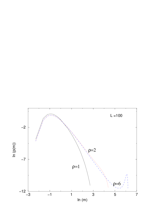
-
1.
When , where and is a normalisation constant for . This is the fluid phase where decays exponentially for large enough
-
2.
When , . This is the critical point where decays as a power law. The critical density is given by
(8) -
3.
When , for finite but large , develops an additional bump centred at . Roughly speaking, for large , . This is the condensed phase where this extra piece of , , emerges in addition to the critical point distribution. This piece (the bump in ) carries a weight . It thus represents a single site containing the excess mass , which coexists with a background of power-law distributed critical mass. The large system-size behaviour of the bump was determined [23, 24] and shown to have distinct forms in the regimes , where on the scale it is gaussian, and , where the distribution is highly asymmetric and non-gaussian. These two forms imply that the number of particles in the condensate has fluctuations of for but anomalously large fluctuations of for .
This description of condensation has been from the point of view of the marginal distribution [23, 24] in the thermodynamic (large ) limit. However, condensation is a co-operative behaviour resulting in the emergence of a single extensive mass amongst the masses. While the signature of the condensation transition is manifest in the single-site mass distribution , a more direct and somewhat natural probe for the condensation is the study of the statistics of the maximal mass in the system. This is because in the condensed phase, the site where condensation occurs is also the site carrying the maximal mass. It is from this perspective, that of the extreme value statistics of the masses, that we study condensation in this work.
2 Condensation and extreme value statistics
In this paper we ask the question—what is the distribution of the largest mass in the system? Thus rather than the single-site mass distribution studied previously, we consider the probability that the largest mass in the system (of size and total mass ) is less than or equal to , which is an example of an extreme value distribution.
In the zero-range process the asymptotic size of the largest mass has been considered by Jeon et al [20]. In that work the case (6) was considered with and it was shown that in the fluid phase , at the critical density , and in the condensed phase . Here we study the statistics of the maximal mass in the more general mass transport model described in the introduction. Moreover, we obtain the full asymptotic probability distribution of the maximal mass for large and not just its average size.
The theory of extreme value statistics (EVS) is well understood for the case of independent random variables. If one considers a set of independent and identically distributed (i.i.d) random variables, each drawn from a common distribution then the limiting distribution of their maximum, appropriately centred and scaled, has three possible forms [26]. The limiting distribution is: a Gumbel distribution when unbounded and decays faster than a power law for large ; a Fréchet distribution when is unbounded and decays as a power law for large , and a Weibull distribution when is bounded.
In our case, however, the masses are correlated due to the global constraint of conserved total mass, explicitly manifest in the delta function in (1). Had this delta function constraint been not there, since , one would expect a Fréchet distribution for the maximal mass based on the EVS of i.i.d. random variables. Here, we find that the delta function induces nontrivial correlations that modify this naive expectation based on the EVS of i.i.d. random variables.
We shall show that the three phases (respectively for , and ) exhibit distinct forms for , the cumulative probability distribution for the largest mass. In the fluid phase ( , appropriately centred and scaled, is a Gumbel distribution; at the critical point () it becomes a Fréchet distribution; in the condensed phase () the distribution of the largest mass in the system is given by where was computed explicitly in [23, 24]. In the latter case we see that maximal mass distribution is essentially given by the tail of the single-site mass distribution. The multiplying factor simply denotes the fact that any of the sites can carry the maximal mass. Thus, in the condensed phase, the maximal mass distribution is neither of the three types (Gumbel, Fréchet or Weibull) that one encounters in the EVS of i.i.d random variables, indicating strong effects of the correlations between the masses. Thus the correlation arising from the global mass conservation modifies the maximal mass distribution both in the fluid phase () as well as in the condensed phase (). Interestingly exactly at the critical point , the maximal mass distribution is Fréchet as would be prediction based on i.i.d variables indicating that the correlation is somehow least effective exactly at the critical point.
3 Computation of the distribution of the largest mass
We begin by defining the cumulative distribution , the probability that the largest mass is less than or equal to :
| (9) |
Here,
| (10) |
and (2) is given by . Equation (9) follows from the fact that if the largest mass is , all masses must be . We shall also consider the probability density of the largest mass
| (11) | |||||
| (12) |
Expression (12) may be compared to the single site mass distribution studied in [23, 24]
| (13) |
The Laplace transform of is easy to compute from (10)
| (14) |
therefore
| (15) |
where and is chosen so that integration contour is to the right of any singularity of the integrand. Our task now is to evaluate the integral (15). In [23, 24] the partition function was evaluated and we shall follow a similar approach here.
3.1 Fluid phase
First we consider the fluid phase in which case may be evaluated by the saddle-point method. Let us define
| (16) |
where due to our choice of normalisation in (6), .
For and large, is asymptotically
| (17) |
On the other hand, for and for large , we have for large ,
| (18) |
Next, using , we may write (15), for large , as
| (19) |
and to leading order the saddle point, , of the integrand is independent of and is given by the equation
| (20) |
where we have used . The saddle point exists and lies on the positive real axis when given from (8) by
| (21) |
Therefore, in the fluid phase (), to leading order, we obtain
| (22) |
where , and we have used (17). For this may be written in the familiar form of a Gumbel distribution
| (23) |
where
| (24) |
Thus the probability density of the maximal mass has a peak around with a width . The scaling form of the distribution around this peak has the Gumbel form (23) and implies that the largest mass is .
3.2 Critical density
3.3 Condensed phase
We now turn to the condensed phase where . In this case the saddle-point method can no longer be used to evaluate (15) as there is no longer a solution to (20).
It turns out to be convenient, in this case, to work directly with the probability density of the largest mass in (12), rather than the cumulative distribution . In fact, the calculation of (12) reduces to precisely that of the distribution detailed in [23, 24] which we now review.
To analyse (12), we need to consider both (in the numerator) and also (in the denominator).
First, the behaviour of for has been computed in [23, 24]. The integral (15)
| (27) |
will be dominated by small values of . Therefore, one expands the term for small. The expansion depends on the value of and is given by
| (28) | |||||
| (29) |
where , and is given by (25).
Similarly, we consider the numerator in (12), for which the relevant integral (15) is
| (30) |
where for large (we will be considering in the large limit)
| (31) |
We now expand this expression for for small , using (28,29).
As a result of the small large , small expansions just described, one obtains from (12)
| (32) |
where has different forms according to the cases and which we discuss separately below.
We note that (32) yields the same leading large behaviour for
as for the single site mass distribution computed in
[24]. This is due to the fact that for the same leading
behaviour is obtained for as for . Moreover,
we can identify the peak in the probability density of the largest mass with
the peak in the single site distribution.
Case (i)
In this case in (32) is given by
| (33) |
The important behaviour of the function determined in [23, 24] may be summarised as
| (34) | |||||
| (35) |
from which we deduce that for
| (36) |
Thus the probability density of the maximal mass is peaked around and near this peak, that is, over a scale of ), the probability density has a normalized gaussian form
| (37) |
Case (ii)
From (12)
one obtains (32)
where now
| (38) |
and
| (39) |
with, as before, . The function is highly asymmetric around and has the following asymptotic behaviour [23, 24]
| (40) | |||||
| (41) |
where and are two constants that were computed in [24]
| (42) | |||||
| (43) |
Using (38) and (40) in (32), we obtain the normalized maximal mass density
| (44) |
Thus, in the condensed phase () the maximal mass distribution has neither of the three forms associated with the EVS of i.i.d random variables. Rather, the scaled distribution has a gaussian form for and has a nontrivial non-gaussian form for . In both cases the largest mass is .
4 Discussion
In summary, we have probed the condensation transition in a generalized class of mass transport models by studying the cumulative probability distribution of the maximal mass in the system. The masses in this model are globally constrained via the mass conservation law. Without this global constraint the masses would have been independent random variables each drawn from a power-law distribution and based on the EVS of the i.i.d random variables one would expect a Fréchet distribution for the maximal mass for all densities . Instead, we have shown via exact asymptotic calculation that the global constraint is sufficiently strong to modify this expectation based on i.i.d. variables and one obtains respectively a Gumbel distribution (for ), a Fréchet distribution (for ) and a completely different distribution in the condensed phase (for ). In the latter case, the distribution is gaussian for and highly non-gaussian for . Thus, our exact results for this model form a useful addition to the list of exactly solvable cases for the distribution of extreme values of a set of correlated random variables, for example, the eigenvalues of random matrices [27, 28, 29, 30, 31, 32], energies of configurations a directed polymer in a random medium [33], the heights in a one-dimensional interface [34, 35, 36, 37]. We note that the Gumbel distribution emerging out of a global constraint was also observed recently in the context of complex chaotic states [38].
We have also seen how in the condensed phase the bump, in the single-site mass distribution is directly related to the probability density of the size of largest mass in the system.
Finally, we note that as the density is increased the phenomenon of condensation is manifested through changes in the asymptotic behaviour of the large mass distribution as described above. It would be of interest to analyse more closely the crossovers, both from the Gumbel distribution for to the Fréchet distribution at and from the Fréchet distribution at to the condensed phase distribution for , as the density is increased. This would involve the consideration of finite-size effects and finite-size scaling near the transition.
References
References
- [1] M. R. Evans, S.N. Majumdar, and R. K. P. Zia, J. Phys. A: Math. Gen 37 (2004) L275
- [2] O.J. O’Loan, M.R. Evans and M.E. Cates, Phys. Rev. E 58, 1404 (1998).
- [3] J Kaupuzs, R Mahnke, RJ Harris, Phys. Rev. E 72, 056125 (2005)
- [4] D. van der Meer, K. van der Weele, P. Reimann and D. Lohse J. Stat. Mech.: Theor. Exp., P07021 (2007); J. Torok. Physica A 355 374 (2005).
- [5] Y. Kafri, E. Levine, D. Mukamel, G.M. Schütz and J. Török, Phys. Rev. Lett. 89, 035702 (2002).
- [6] S. N. Dorogovtsev and J.F.F. Mendes, Evolution of Networks (OUP, Oxford, 2003)
- [7] A. G. Angel, M. R. Evans, E. Levine, D. Mukamel Phys. Rev. E, 72, 046132 (2005)
- [8] A. G. Angel, T. Hanney, and M. R. Evans, Phys. Rev. E 73, 016105 (2006)
- [9] S.N. Coppersmith, C.-h. Liu, S. Majumdar, O. Narayan, T.A. Witten, Phys. Rev. E., 53, 4673 (1996).
- [10] S.N. Majumdar, S. Krishnamurthy and M. Barma, Phys. Rev. Lett. 81, 3691 (1998); J. Stat. Phys. 99, 1 (2000).
- [11] J. Krug and J. Garcia, J. Stat. Phys., 99 31 (2000); R. Rajesh and S. N. Majumdar, J. Stat. Phys., 99 943 (2000).
- [12] E. Bertin, J. Phys. A: Math. Gen. 39, 1539 (2006).
- [13] M. R. Evans and T. Hanney, J. Phys. A: Math. Gen. 38, R195 (2005)
- [14] F. Zielen and A. Schadschneider, Phys. Rev. Lett 89 090601 (2002)
- [15] R. K. P. Zia, M. R. Evans, S.N. Majumdar, J. Stat. Mech. : Theor. Exp. (2004) L10001.
- [16] M. R. Evans, S.N. Majumdar, and R. K. P. Zia, J. Phys. A: Math. Gen 39, 4859-4873 (2006)
- [17] J. Walrand An Introduction to Queueing Networks (Prentice-Hall, 1988)
- [18] P. Bialas, Z. Burda, and D. Johnston, Nucl. Phys. B 493, 505 (1997).
- [19] M.R. Evans, Braz. J. Phys. 30, 42 (2000).
- [20] I. Jeon, P. March and B. Pittel, Ann. Prob. 28 1162 (2000)
- [21] S. Großkinsky, G.M Schütz and H. Spohn, J. Stat. Phys 113, 389 (2003).
- [22] C. Godrèche, J. Phys. A: Math. Gen., 36, 6313 (2003).
- [23] S.N. Majumdar, M. R. Evans, and R. K. P. Zia, Phys. Rev. Lett. 94, 180601 (2005)
- [24] M. R. Evans, S.N. Majumdar, and R. K. P. Zia, J. Stat. Phys. 123 357 (2006)
- [25] P. A. Ferrari, C. Landim, and V. V. Sisko, J. Stat. Phys 128 1153 (2007)
- [26] E.J. Gumbel, Statistics of Extremes (Columbia University, New York, 1958).
- [27] A. Edelman, Siam J. Matrix Anal. Appl. 9, 543 (1988).
- [28] C.A. Tracy and H. Widom, Commun. Math. Phys. 159, 151 (1994).
- [29] K. Johansson, Comm. Math. Phys. 209, 437 (2000).
- [30] I.M. Johnstone, Ann. Stat. 29, 295 (2001).
- [31] G. Biroli, J.-P. Bouchaud, and M. Potters, Europhys. Lett. 78, 10001 (2007).
- [32] S.N. Majumdar, O. Bohigas, and A. Lakshminarayan, J. Stat. Phys. 131, 33 (2008).
- [33] S.N. Majumdar and P.L. Krapivsky, Phys. Rev. E 62, 7735 (2000); D.S. Dean and S.N. Majumdar, Phys. Rev. E 64, 046121 (2001).
- [34] G. Gyorgyi et. al. Phys. Rev. E 68, 056116 (2003).
- [35] S.N. Majumdar and A. Comtet, Phys. Rev. Lett. 92, 225501 (2004); J. Stat. Phys. 119, 777 (2005).
- [36] G. Schehr and S.N. Majumdar, Phys. Rev. E 73, 056103 (2006).
- [37] G. Gyorgyi, N.R. Maloney, K. Ozogany, and Z. Racz, Phys. Rev. E 75, 021123 (2007).
- [38] A. Lakshminarayan, S. Tomsovic, O. Bohigas, and S. N. Majumdar, Phys. Rev. Lett. 100, 044103 (2008).