The limb-darkened Arcturus

Abstract

Aims. This paper is an H band interferometric examination of Arcturus, a star frequently used as a spatial and spectral calibrator.

Methods. Using the IOTA 3 telescope interferometer, we performed spectro-interferometric observation ($R\approx 35$) of Arcturus. Atmospheric models and prescriptions were fitted to the data to derive the brightness distribution of the photosphere. Image reconstruction was also obtained using two software algorithms: Wisard and Mira.

Results. An achromatic power law proved to be a good model of the brightness distribution, with a limb darkening compatible with the one derived from atmospheric model simulations using our marcs model. A Rosseland diameter of $21.05\pm 0.21$ was derived, corresponding to an effective temperature of $T_{\rm eff}=4295\pm 26$ K. No companion was detected from the closure phases, with an upper limit on the brightness ratio of $8\times 10^{-4}$ at 1AU. Dynamic range at such distance from the photosphere was established at $1.5\times 10^{-4}$ ($1\sigma\,$rms). An upper limit of $1.7\times 10^{-3}$ was also derived for the level of brightness asymmetries present on the photosphere.

1 Introduction

Arcturus’ curse is to be too popular. Many new generations of instruments – including interferometers – observe it as a test object. The reasons for that: this red giant is bright, large, and spectrally well-defined. The curse is: since the instruments are new, the star usually takes face on the bizarre systematic errors of challenging observations. We can cite, among others, inexact diameter and temperature measurements (prompting Griffin & Lynas-Gray (1999) to write an article entitled “The Effective Temperature of Arcturus”), or false duplicity observations (“Arcturus as a Double Star” by Griffin 1998).

This paper does not pretend to be an exception – interferometry is still a challenging technique. The main difference is in the interferometer used: at the time of our observations, IOTA was more wise than new (we shall note that Arcturus has already been observed several times by IOTA and led to three different publications; Dyck et al. 1996; Perrin et al. 1998; Verhoelst et al. 2005). The initial goal of a new observation run was to leverage the more extended capability of IOTA to show the ability of the interferometer to do a reliable image of a commonly observed object.

Indeed, image reconstruction is difficult. Even though it is routinely performed by the current generation of radio interferometers, this technique – herein called “regularized imaging” – remains marginal in optical interferometry. This is simply due to a lack of spatial frequency coverage. Optical interferometers are usually more difficult to build, and the complexity quickly increases with the number of telescopes. Therefore, since the amount of information accessible in the Fourier plane is sparse, our ability to reconstruct a reliable image of a complex object is limited.

A more common data analysis is to suppose the object to be conform to a model – or prescription. Originally, it consisted in fitting visibility curves of uniform disks (e.g. Michelson & Pease 1921; di Benedetto & Foy 1986). With time, it included more complicated models, e.g. limb-darkened disks (e.g. Quirrenbach et al. 1996, MkIII), disks with spots (e.g. Young et al. 2000, COAST), disks with a molecular envelope (e.g. Perrin et al. 2004, IOTA), etc. Both methods, regularized imaging and model fitting, complement each other. The role of regularized imaging is commonly to guide the choice and complexity of a model. The role of model fitting is to obtain the highest precision results on the parameters of the model. The pitfall may be when the model does not best suit the object, hence the need for quality regularization imaging.

Recently the maturation of interferometric facilities (e.g. IOTA, CHARA, VLTI) reached the point where $u$-$v$ coverage (both in amplitude and phase) allows regularized imaging (Monnier et al. 2007a; Lacour 2007). Here we present the data on Arcturus, used as a test star for optical interferometry reconstruction softwares. Several astrophysical issues also justify this investigation: 1) what is the limb darkening? Is it compatible with red giant atmosphere modeling (Davis et al. 2000; Claret 2000)? 2) are the disputed previous detections of a companion compatible with our observations (Perryman et al. 1997; Verhoelst et al. 2005; Brown 2007)?

The outline of this paper is as follows. Section 2 gives an overview of the IOTA interferometer, describes the data reduction process and shortly present the dataset. Section 3 compares our data with atmosphere models, using either limb-darkening prescriptions or a more evolved atmospheric simulation (the Marcs model). Section 4 investigates on a possible deviation from point symmetry. Results of image reconstruction are presented in Section 5, and Section 6 conclude.

2 Observation and data reduction

2.1 Description of IOTA observations

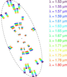
Figure 1: $u$-$v$ coverage. Maximum projected baseline length is 37.7 meters. The lack of high frequency information in the East-West direction is due to the geometry of IOTA.

Figure 2: Single scan obtained on calibrator HD 120477. It shows the flux (arbitrary units) as a function of the optical path difference (OPD) for the three baselines, and the seven spectral channels. Eye inspection allows to observe the decreasing frequency – and therefore increasing wavelength – from top to bottom. The bottom fringes correspond to the sum of the spectral channels, showing a radical change in the coherence length. Each datapoint is composed of 200 scans.

The interferometric data presented herein were obtained using the IOTA (Infrared-Optical Telescope Array) interferometer (Traub et al. 2003), a long baseline interferometer which operates at near-infrared wavelengths. It consists of three 0.45 meter telescopes movable among 17 stations along two orthogonal linear arms. IOTA synthesizes a total aperture size of $35\times 15\,$m, corresponding to an angular resolution of $\approx 10\times 23$ milliarcseconds at 1.65 $\mu$m. Visibility and closure phase measurements were obtained using the integrated optics combiner IONIC (Berger et al. 2003); light from the three telescopes is focused into single-mode fibers and injected into the planar integrated optics (IO) device. Six IO couplers allow recombinations between each pair of telescopes. Fringe detection is done using a Rockwell PICNIC detector (Pedretti et al. 2004). The interference fringes are temporally-modulated on the detector by scanning piezo mirrors placed in two of the three beams of the interferometer.

Observations were undertaken in the H band ($1.5\,\mu$m$\,\leq\,\lambda\leq\,1.8\,\mu$m) divided into 7 spectral channels. The science target observations are interleaved with identical observations of unresolved or partially resolved stars, used to calibrate the interferometer’s instrumental response and effects of atmospheric seeing on the visibility amplitudes. The calibrator sources were chosen in two different catalogs: Bordé et al. (2002) and Mérand et al. (2006); using criteria on the separation ($\lesssim 10$ degrees) and magnitude. The calibrators are listed in Table 1.

Table 1: Calibrators

	Calibrator	Spectral Type	UD diameter
1	HD 120477	K5.5 III	$4.460\pm 0.050$
2	HD 125560	K3 III	$1.910\pm 0.021$
3	HD 129972	G8.5 III	$1.540\pm 0.020$

Arcturus was observed in May 2006 during 5 nights and using 5 different configurations of the interferometer. Full observation information can be found in Table 2, including dates of observation, interferometer configurations and calibrators. Fig. 1 shows the $u$-$v$ coverage achieved during this observation run. The geometry of the IOTA interferometer and the position of the star on the sky constrained the extent of frequency coverage. We covered a frequency range equivalent to the one of an elliptical telescope of aperture $38\times 15$ meters, with a 20 degree inclination East of North.

Table 2: Arcturus observing log

Date	Interferometer	Calibrator
(UT)	Configurationa	(Table 1)
2006 May 11	A15-B05-C10	1, 2, 3
2006 May 12	A15-B05-C00	1, 2, 3
2006 May 13	A15-B15-C00	1, 3
2006 May 14	A30-B15-C00	2
2006 May 16	A35-B15-C25	2, 3

• Configuration refers to the location in meters of telescopes A, B, C on the NE, SE and NE arms respectively.

2.2 Data reduction

Reduction of the IONIC visibility data was carried out using custom software similar in its main principles to the one described by Coude Du Foresto et al. (1997). We measured the power spectrum of each interferogram (proportional to the target squared visibility, $V^{2}$), after correcting for intensity fluctuations and subtracting bias terms from read noise, residual intensity fluctuations, and photon noise (Perrin 2003). Next, the data pipeline applies a correction for the variable flux ratios for each baseline by using a flux transfer matrix (Monnier 2001). Finally, raw squared visibilities are calibrated using the raw visibilities obtained by the same means on the calibrator stars. Calibration accuracy had been studied by extensive observation of the binary star $\lambda$ Vir. For bright stars (H mag $\lesssim 5$), Zhao et al. (2007) have validated 2 % calibration error for $V^{2}$; corresponding to a 1% error in visibility. We therefore systematically added a 2% calibration error on all the squared visibilities present in this paper.

In order to measure the closure phase (CP), a fringe tracking algorithm was applied in real-time while recording interferograms (Pedretti et al. 2005), ensuring that interference occurs simultaneously for all baselines. We required that interferograms are detected for at least two of the three baselines in order to assure a good closure phase measurement. This technique, called “baseline bootstrapping” allowed precise visibility and closure phase measurements for a third baseline with very small coherence fringes. We followed the method of Baldwin et al. (1996) for calculating the complex triple amplitude and deriving the closure phase. Pair-wise combiners (such as IONIC) can have a large instrumental offset for the closure phase which requires to be calibrated by the closure phase of the calibrator stars. We noticed very stable closure phase measurements during the nights with drifts of less than a degree.

2.3 Wavelength calibration

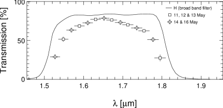
Figure 3: Relative photometry between the different spectral channels as a function of the wavelength (arbitrary vertical units). The wavelength was determined by measuring the frequency of the fringes as shown in Fig. 2.

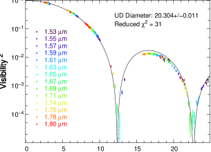
Figure 4: Overview of the dataset: Visibility square measurements as a function of the baseline length. The wavelength is color coded with the same palette used in Fig. 1. The solid curve correspond to the visibility curve of a uniform stellar disk of angular diameter 20.30 mas (not accounting for bandwidth smearing). The bottom panel presents the residual of that fit, showing the clear inconsistency of the second lobe.

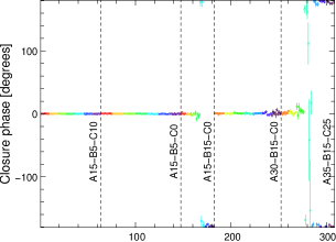
Figure 5: Overview of the dataset: closure phase measurement as a function of observation datafile number. The bottom panel shows the residual of fitting a simple limb darkening disk to the data (power law with parameters as stated in Table 3). Color legend is similar to the one used in Fig. 1 and 4. Because such a model corresponds to a symmetrical brightness distribution, the closure phases are either 0 or 180 degrees. The reduced $\chi^{2}$ of the closure phase alone is 1.06.

Spectral information was obtained by the means of a prism placed between the integrated optics and the PICNIC camera (Ragland et al. 2003). The temporally-modulated fringes are therefore spatially dispersed on the detector. To ensure well-defined spectral edges, we also inserted a broad band H filter in the optical path. Its bandpass is spatially equivalent to seven pixels on the camera.

Wavelength calibration of the spectral channels is however a difficult and critical step. This is especially important since the prism was removed and re-inserted (with a slightly different position) between the night of the 13th and the 14th. Fortunately, the spectral wavelength is coded in the data (see Fig. 2). The fringe frequency (in pixels^-1) is directly proportional to the wavenumber. The factor of proportionality is constant since the modulation of the optical path is done by moving the piezo mirrors a certain distance (step-like) between each pixels reads, even though the steps are smoothed out by mirror/mount inertia. The relative wavelength between each channel and each night was established this way with a precision better than $0.1\%$. This level of precision was achievable thanks to small differential piston variations due to good seeing conditions and fast reading mode. The relative wavelength between each baseline was also studied. To do so, we compared the fringe frequency observed at a given spectral channel between the three baselines. The frequency of the third baseline is equal to the sum of the frequency of the two first, within $0.2\%$ error bars. This means that the different baselines are at equal wavelength at a $0.2\%$ level.

However, absolute calibration requires to know the exact angle of the incoming beam on the piezo mirror. March 2007 narrow band observations were used, and allowed to establish the speed of the optical path modulation at $0.188\pm 0.002\,\mu$m/sample for the first delay line, and $0.195\pm 0.002\,\mu$m/sample for the second delay line. Optical path modulation was measured on the third baseline at $0.383\pm 0.004\,\mu$m/sample. A time sample correspond to the integration time between two reads. The $\approx 1\%$ error bars are mainly due to uncertain changes in the angle of reflection which occurred between March and May 2006.

Figure 3 summarizes the wavelength calibration results by plotting the average integrated flux on each spectral channel as a function of wavelength. The fairly large error bars in wavelength are mainly due to the uncertainty on the angle of reflection, and correspond to a possible global shift in absolute calibration. In contrast, relative wavelength is precisely established, and shows that a significant displacement of the prism occurred between the night of the 13th (squares), and the night of the 14th (cross).

2.4 IOTA field of view

The high resolution of IOTA has a counterpart: the field of view is limited. The first limitation is due to the field of view of each individual telescopes, delimited by the cone of acceptance of the fibers on the sky. Such value is difficult to estimate, since it depends on the interferometer as well as the atmospheric seeing. A first order estimation is to neglect the atmospheric turbulence and to consider the fiber core to be filling the diffraction pattern of the telescopes. In this assumption, the field of view of the telescopes reads:

$$FOV_{\rm telescopes}=\frac{\lambda}{D}\,,$$ (1)

where D is the diameter of an individual telescope.

A second limitation is the field of view of the interferometer. It is delimited by the maximum distance between two objects which fringes overlap on the detector. To be rigorous, one should take into account parameters like the mode of recombinaison, the stroke of the piezo (in the case of IONIC), and even the spectral energy distribution of the target. However, to establish a simple relation, we will only take into account the spectral bandwidth of a spectral channel ($\Delta\lambda$), as well as the distance between two telescopes ($B$):

$$FOV_{\rm interferometer}=\frac{\lambda^{2}}{\Delta\lambda\,B}\,.$$ (2)

Note that the interferometric field of view is baseline dependent. It will be larger for shorter baselines, and smaller for longer baselines. Moreover, this field limitation is valid only in the direction along the baseline. Perpendicular to the baseline, the bandpass does not cause any field limitation. All in all, it is difficult to establish the field of view of an interferometer as a whole. A conservative way to do so is to consider the maximum baseline length for a given direction.

In the North-East/South-West direction, using the spectral dispersion mode of IOTA ($D=45$ cm, $\Delta\lambda=40$ nm and $B=35$ m), the field of view is not limited by the telescope ($FOV_{\rm telescopes}=750$ mas), but by the bandwidth. The field of view is 350 mas at 1.55 $\mu$m, and 480 mas at 1.80 $\mu$m. In the North-West/South-East direction, the shorter baselines ($B=15$ m) allow a larger interferometric field of view, hence a 750 mas field limitation due to the telescopes size.

We will consider in the following of this paper a 400x750 mas field of view for IOTA.

2.5 The dataset

The dataset consist of 924 visibility measurements and 308 closure phases. The $V^{2}$ are plotted as a function of the baseline length in the upper panel of Fig. 4. The CP are plotted in the upper panel of Fig. 5. The frequency plane coverage was previously presented in Fig. 1. The solid curve corresponds to the best fit of a uniform disk. The residuals are plotted on the lower panels. It is interesting to note that fringes have been observed with a contrast below 1%. Such a low contrast exists thanks to the dispersive mode, which allows a deep first null. If the full H band was observed, the effect of bandwidth smearing would have limited the depth of the null to several percents (Perrin & Ridgway 2005). Probing into the null was possible thanks to bootstrapping, two baselines of sufficient contrast being enough to track the fringes on all the baselines.

A few things are striking: first, the object is relatively achromatic. This can be seen on the residuals of the $V^{2}$. Secondly, the second lobe of the data is not well fitted by a uniform disk. This is due to the presence of limb darkening. Thirdly, the closure phases are close to zero or $\pi$. It means the object is likely to be point symmetric.

3 Comparison with atmosphere models / prescriptions

3.1 Fitting limb-darkening prescriptions

Table 3: Diameter and limb darkening measurements

Law	parameters	Reduced $\chi^{2}$
Uniform	$\theta_{\rm UD}=20.304\pm 0.011$ mas	31
Power	$\theta_{\rm LD}=20.900\pm 0.007$ mas	1.962
	$\alpha=0.258\pm 0.003$
Quadratic	$\theta_{\rm LD}=20.922\pm 0.036$ mas	1.959
	$a=0.186\pm 0.021$
	$b=0.298\pm 0.053$
Quadratic	$\theta_{\rm LD}=20.931\pm 0.004$ mas	2.956
Claret (2000)	$a=0.0291$
	$b=0.5107$
Non-linear	$\theta_{\rm LD}=20.863\pm 0.004$ mas	2.013
Claret (2000)	$a_{1}=0.8175$
	$a_{2}=0.0827$
	$a_{3}=-0.4116$
	$a_{4}=0.1864$
marcs model	$\theta_{\mathrm{Ross}}=21.05\pm 0.01$ mas	2.080

• Errors bars are pure calculations based on the second derivate of the $\chi^{2}$. They are not valid when assuming an unrealistic model of the brightness distribution (for example a uniform disk). Moreover, diameter errors do not include the 1% uncertainty due to an eventual wavelength miscalibration (see section 2.3).

Since limb darkening is apparent, a logical first step is to fit a model for the brightness distribution of the photosphere. Numerous types of limb-darkening (LD) prescriptions exist in the literature. We used two of them, which we supposed achromatic. A power law (Hestroffer 1997):

$$I(\mu)/I(1)=\mu^{\alpha}\,,$$ (3)

and a quadratic law (Manduca et al. 1977):

$$I(\mu)/I(1)=1-a(1-\mu)-b(1-\mu)^{2}\,,$$ (4)

where $\mu=\sqrt{1-(2r/\theta_{\rm LD})^{2})}$, $r$ being the angular distance from the star center, and $\theta_{\rm LD}$ the angular diameter of the photosphere. In terms of complex visibilities, the power law limb darkening prescription yields:

$$V(v_{r})=\sum_{k\geq 0}\frac{\Gamma(\alpha/2+2)}{\Gamma(\alpha/2+k+2)\Gamma(k+1)}\left(\frac{-(\pi v_{r}\theta_{\rm LD})^{2}}{4}\right)^{k}\,,$$ (5)

where $v_{r}$ is the radial spatial frequency and $\Gamma$ the Euler function ( $\Gamma(k+1)=k!$). On the other hand, the quadratic law yields:

$$V(v_{r})=\frac{\displaystyle(1-a-b)\frac{J_{1}(\zeta)}{\zeta}+\frac{a+2b}{\sqrt{2/\pi}}\frac{J_{3/2}(\zeta)}{\zeta^{3/2}}-2b\frac{J_{2}(\zeta)}{\zeta^{2}}}{\displaystyle{1/2}-{a/6}-{b/12}}$$ (6)

where $\zeta=\pi v_{r}\theta_{\rm LD}$, $J_{1}$ and $J_{2}$ are the first and second-order Bessel function respectively, and:

$$J_{3/2}(\zeta)=\sqrt{\frac{2}{\pi\zeta}}\left(\frac{\sin(\zeta)}{\zeta}-\cos(\zeta)\right)\,.$$ (7)

Results for the fits are presented in Table 3. Using Eq. (3), we obtained a $\chi^{2}$ of 2413, for 1230 degrees of freedom. The reduced $\chi^{2}$ ($\chi^{2}$ over the number of degrees of freedom) does not improve significantly when using a two-parameter prescription for limb darkening, prompting us to consider the power law model as a sufficient approximation.

There are two main explanations for the reduced $\chi^{2}$ different from one: (i) an underestimation of the error bars, and (ii) an inexact prescription of the brightness distribution by Eqs. (3) and (4). Making the distinction between these two is difficult. On the one hand, photometric variations of the star are observed at the order of one percent (Retter et al. 2003), an indication that the brightness distribution should not be as smooth and symmetric as our prescriptions are. On the other hand, no deviation from point symmetry is observed in the closure phases (section 4) whose reduced $\chi^{2}$, taken independently, is 1.015. The departure from simple LD models could therefore only be explained by a missing point-symmetric component. The residuals are discussed more throughly in the last paragraph of Section 3.2.

Whatever the cause, we decided to be as conservative as possible by scaling the errors to a $\chi^{2}$ of one. The error bars stated in Table 3 are obtained by this mean. To decrease the $\chi^{2}$, we explored – and discarded – two other alternatives. The first one was to increase the error due to calibration (higher than the 2% justified in section 2.2). However, this dramatically increased the errors bar on the lowest frequencies, which is not desired since they are already well fitted by our prescriptions. The second approach was to add an additive error due to a potentially imperfect subtraction of the power spectrum bias. Such an error was included at a 2% level for faint objects by Monnier et al. (2006). However, this dramatically increased the errors bars on the lowest visibilities, which brings an unnecessary bias on data whose first zero is already well fitted. In conclusion, a global scaling of the error bars was seen as the best alternative.

3.2 Fitting the Marcs model

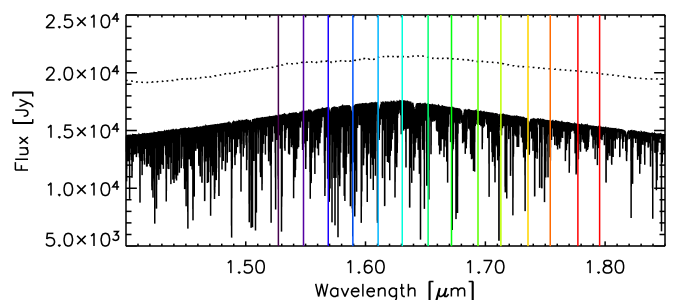
Figure 6: The synthetic H-band spectrum of the marcs model (solid line: in opacity sampling resolution, dotted line: convolved to the instrumental spectral resolution – shifted up by five thousands Jensky) and the central wavelengths of the spectral channels of IONIC. The peak in the spectrum corresponds to the H^- opacity minimum.

Figure 7: Wavelength dependent visibility curves derived from the Marcs atmospheric model. The color coding is similar to the one used in Fig. 6. IONIC data are superimposed on the curves, and residuals are plotted in the lower panel. The closure phase residuals are identical to those of Fig. 5.

The Marcs atmospheric model was presented in Verhoelst et al. (2005). The models were originally constructed and fine-tuned for the calibration of the ISO-SWS (Infrared Space Observatory Short Wavelength Spectrometer) and checked against FTS spectra (Decin 2000). For the present study, we searched the full Arcturus FTS spectral atlas (Hinkle et al. 1995) in the H band for peculiar spectral features. Lines are sparse and well spaced. They belong mainly to CN, OH and some atomic transitions. The IONIC data are therefore ideal to study the H^- continuum, which has its minimum (the transition between bound-free and free-free regimes) within the bandpass sampled by our data. The only free parameter to match model to observations is the angular diameter corresponding to the outermost point in our model intensity profiles ($\tau_{\mathrm{Ross}}=10^{-7}$). Several models with stellar parameters around those determined by Decin et al. (2003) were used, but they bring no significant improvement in $\chi^{2}$ compared to the spectroscopically preferred model (T${}_{\rm{eff}}=4320\,$K, $\log{g}=1.5$, [Fe/H] = -0.5 and v${}_{\rm{turb}}=2$ km s^-1).

The synthetic H-band spectrum calculated from our model and the comparison of our dataset with this model are shown in Fig. 6 and Fig. 7. We find the best agreement for a diameter of $21.465\pm 0.008$ mas, which corresponds to a $\tau_{\mathrm{Ross}}=1$ diameter of 21.05 mas. This diameter is slightly larger than the one found in Sect. 3.1: the star appears a little smaller at wavelengths of minimal photospheric opacity than at the Rosseland-averaged opacity.

With a $\chi^{2}$ of 2, this fit is almost as good as it was when fitting a free-parameter limb darkening prescription. This is an overall confirmation of the validity of the Marcs modeling of the limb darkening. Analysis of the visibility residuals plotted in Fig. 7 indicates some possible shortcomings of the model (supposing error bars are not underestimated, see Section 3.1). Indeed, the high $\chi^{2}$ can be accounted for by two biases: a chromatic bias at low frequency ($\approx 9\,$M$\lambda$), another achromatic at high frequencies (around the second nul). Accounting for these biases could be done by (i) introducing a circumstellar emission of H₂O at a level of half a percent (water detection was reported by Ryde et al. 2002, although normal hydrostatic model does not predict any in the photosphere), and (ii) slightly modifying the limb darkening distribution. However, such possibilities are at the limit of what we think is reasonable to derive from our data, and no further modeling was done to avoid over-interpretations.

3.3 On the angular diameter of Arcturus

Numerous angular diameter measurements can be found in the literature. Previous interferometric observations either use uniform-disk fitting and apply limb-darkened corrections, or fit disks whose limb-darkening is fixed by atmospheric models. At a wavelength of $2.2\mu$m, di Benedetto & Foy (1986) observed Arcturus with the I2T interferometer and published a diameter of $\theta_{\rm UD}=20.36\pm 0.20$ mas as well as a limb-darkened value $\theta_{\rm LD}=20.95\pm 0.20$ mas. Previous measurements using the IOTA interferometer exist too, and yielded in the K band $\theta_{\rm LD}=19.5\pm 1.0$ mas (Dyck et al. 1996, using bulk optics), $\theta_{\rm LD}=20.91\pm 0.08$ mas (Perrin et al. 1998, using FLUOR) and $\theta_{\rm Ross}=21.18\pm 0.21$ mas (Verhoelst et al. 2005, also using FLUOR). In the visible, Mozurkewich et al. (2003) observed Arcturus using the MarkIII interferometer (450-800 nm), and after correction for a substantial limb darkening effect, published $\theta_{\rm LD}=21.373\pm 0.247$ mas.

From our dataset, and taking into account wavelength calibration uncertainties, we derived $\theta_{\rm LD}=20.91\pm 0.21$ mas and $\theta_{\rm Ross}=21.05\pm 0.21$ mas. These results are in agreement with I2T, MarkIII and IOTA observations ($1.5\sigma$ in Dyck et al. 1996). It does not yield an increase in terms of precision, but our measurements are indeed interesting since, unlike the others, they did not require a pre-defined value to account for limb darkening. Using the Rosseland diameter and Griffin & Lynas-Gray (1999) estimation of the integrated flux ($F=(4.98\pm 0.02)\times 10^{-5}$ erg cm^-1 s^-1), we can update their calculation of Arcturus’ effective temperature to $T_{\rm eff}=4295\pm 26$ K.

3.4 On the limb darkening

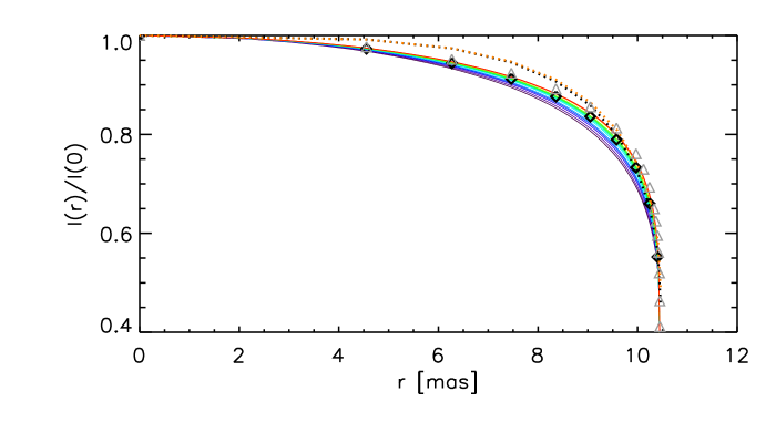
Figure 8: Intensity profiles of our marcs model as colored lines. For comparison, the best parametric fit of a power law is represented with diamonds, the Kurucz model with triangle, and the quadratic LD curve Claret (2000) as a dotted line. This last fit differs significantly form the others, revealing a problem in the method used for limb darkening fitting used by Claret.

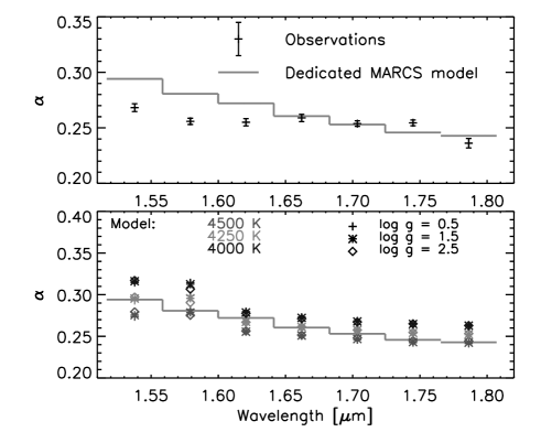
Figure 9: Limb darkening as a function of the wavelength. Upper panel: the observed LD coefficients $\alpha$ (with error bars) are compared with the LD coefficients derived by fitting a $I(\mu)=\mu^{\alpha}$ profile to the Marcs intensity profiles of our dedicated Arcturus model (T${}_{\rm{eff}}=4320\,$K, $\log{g}=1.5$, [Fe/H] = -0.5 and v${}_{\rm{turb}}=2$ km s^-1). Lower panel: influence of temperature and gravity on the limb darkening.

An important prospect of this work was to compare our limb darkening measurements with existing atmospheric models. A first test was to derive parameters of the limb darkening, and compare them with published values in the literature. We were greatly surprised to see a strong inadequacy between our measurements and the quadratic parameters given by Claret (2000) (see Table 3 and Fig. 8). However, they also published the values for a more complex 4-parameter non-linear law:

$$\frac{I(\mu)}{I(1)}=1-a_{1}(1-\sqrt{\mu})-a_{2}(1-\mu)-a_{3}(1-\mu^{3/2})-a_{4}(1-\mu^{2})\,.$$ (8)

Claret (2000) claims that this four-parameter non-linear law should give a more reliable estimation of the limb darkening. Using his published parameters (assuming T${}_{\rm{eff}}=4250\,$K, $\log{g}=1.5$, [Fe/H] = -0.5 and v${}_{\rm{turb}}=2$ km s^-1) we were able to indeed confirm a correct fit.

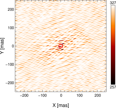
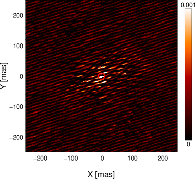
Figure 10: Non-detection of a companion to Arcturus. Left panel: closure phase $\chi^{2}$ map. Right panel: $1\sigma$ upper limits of the brightness ratio of a companion. The circles represent the limit of the photosphere. The field of view of IOTA is 400x750 mas (see discussion in Section 2.4).

However, it is not the quadratic law which is intrinsically less able to match the limb darkening: when leaving the parameters free to adjust, the $\chi^{2}$ of a quadratic law is able to match the $\chi^{2}$ of the non-linear law. Therefore, the problem with the quadratic values published by Claret (2000) should lie in the method to derive the parameters. To confirm this, we used the Atlas model (Kurucz 1979) – the one used by Claret – and we were able to obtain a good fit for the limb darkening (see Fig. 8). An explanation could be found in a paper written by Heyrovský (2007), in which the author states that conventional stellar limb fitting methods (like the one used by Claret) are biased.

But the most striking results from Table 3 is the consistency in fitting quality achieved when using different limb darkening laws (except when using Claret’s quadratic value). We noted that both Marcs and Atlas models give similar fits, showing an equivalent capacity to correctly model the atmosphere of Arcturus. The reduced $\chi^{2}$ values are not exactly 1, but are close to the ones obtained when fitting LD laws with freely variable parameters. This is a good validation of both atmospheric modeling softwares. Secondly, we do not note any difference in the fitting quality between a power and a quadratic limb darkening law. Furthermore, the likelihood does not increase when using a 4-coefficient non-linear law (reduced $\chi^{2}$ of 1.97 – we do not present the results in Table 3 since none of the coefficients are properly constrained by our dataset). This is because we do not have the necessary angular resolution to distinguish the several limb darkening laws used here. To our dataset, all of them are equally good. Therefore, for angular resolution no greater than ours, we recommend using the power law instead of the two other limb darkening laws tested in this work, since it would use less free parameters while still being able to correctly model the LD.

Finally, we investigated the spectral dependence of the limb darkening. To do so, we fitted a limb-darkening power law with a wavelength-dependent $\alpha$ value to the observations. The fit was done using an achromatic diameter as, in principle, there is no such thing as a different diameter at different wavelengths: a different intensity profile, or in the case of a well-behaved star just a different LD, mimics a different diameter at different wavelengths. In the absence of extended molecular layers and other similar large deviations from a normal photospheric IP, this effect is mostly accounted for by the LD parameter. Similarly, we derived theoretical $\alpha$ values from our preferred marcs model. The result is summarized in Fig. 9. The general agreement is quite good. The almost linear slope of the limb-darkening is in fact a complex combination of opacity due to the H^- continuum and molecular absorptions features. A minor discrepancy is an overestimation of the LD at the blue end of the bandpass. We searched a grid of models for possible improvement, but no significantly better fit could be attained with reasonable stellar parameters.

4 On the point symmetry of Arcturus

4.1 Fitting the closure phases

Closure phases (CP) are extremely sensitive to deviations from point symmetric brightness distributions. For example, a binary of contrast ratio 1:100 could induce closure phases of several tens of degrees at low visibilities. The mean of our first 147 CP measurements (first two days of observation) is 0.067 degree, with an average root mean square of 0.34 degree. Such high quality data is therefore excellent for probing a companion. When fitting a power law limb-darkened disk to the data (both $V^{2}$ and CP; see section 3.1), the $\chi^{2}$ on the CP was 327 over 308 closure phases — corresponding to a reduced $\chi^{2}$ of 1.07. Fig. 5 shows the CP as well as the residual of the fit. The fit is, in our opinion, satisfactory.

An upper limit for the brightness ratio of a possible companion can be obtained. We modified the visibility function presented in Eq. (5) to account for the presence of a point-like off-centered source:

$$V(u,v) = (1-K)\sum_{k\geq 0}\frac{\Gamma(\alpha/2+2)}{\Gamma(\alpha/2+k+2)\,k!}\left(\frac{-\pi^{2}\theta_{\rm LD}^{2}(u^{2}+v^{2})}{4}\right)^{k}$$ (9)

$$+K\exp\left(2i\pi(Xu-Yv)\right)\,.$$

$K$ is the brightness ratio of the companion, $X$ and $Y$ its position and $u$ and $v$ the spatial frequencies (arcsec^-1). The star parameters ($\alpha$ and $\theta_{\rm LD}$) are fixed to the value presented in Table 3. For each position of the companion Eq. (9) is computed, CP are derived and $K$ is adjusted to minimize the $\chi^{2}$ on the closure phases. The minimum $\chi^{2}$ are plotted as a function of $X$ and $Y$ on the left panel of Fig. 10. The general minimum $\chi^{2}$ for a companion situated within the field of view of IOTA but further away than 1 AU of the star (400 mas$>\sqrt{X^{2}+Y^{2}}>89$ mas) is 299, with a brightness ratio $K=(4\pm 4)\times 10^{-4}$. This is not significant enough to be considered a detection. The values $(K+\sigma(K))$ can nevertheless be used to derive upper limits for the brightness ratio of a possible binary system. It is plotted in the right panel of Fig. 10. The average dynamic range at 1 AU of the star is $1.5\times 10^{-4}$.

Closer to the photosphere, the $\chi^{2}$ can decrease substantially. The minimum is 257, for $X=10$ and $Y=11$ mas. It still does not mean we have detected anything, since this value is below the number of degrees of freedom. However, the fit can be used to put upper limits on the brightness of a possible hotspot on the photosphere. The maximum value for $K+\sigma(K)$ on the photosphere is $1.7\times 10^{-3}$. Note that the signature of an hotspot on the CP gets smaller when it gets closer to the photocentre. Therefore, we cannot exclude the presence of a bright hotspot coincidentally situated in the middle of the photosphere.

4.2 Presence of a companion?

Arcturus is often used for high-resolution spatial and spectral calibration (Tuthill et al. 2000; Decin et al. 2003). Such use makes this star both very well known and very important to know. This explains why, when Hipparcos flagged this star as a binary, it stirred an important debate in the community. The absence of other observational evidence (Griffin 1998), uncertainties in the Hipparcos detection (Soderhjelm & Mignard 1998) and finally non-detection with adaptive optics observations (Turner et al. 1999), convinced the community they could keep using Arcturus as a calibrator. Our results put an upper limit on the brightness ratio of a possible companion to $8\times 10^{-4}$ in the H band.

To make our results compatible with a binary system as proposed by Hipparcos (Perryman et al. 1997) or Verhoelst et al. (2005) ($\Delta m\approx 4$, $\rho\approx 230$ mas, $M\geq 0.7M_{\odot}$), we would have to imagine either (i) a strong dependence of the wavelength or (ii) an edge-on orbit with the secondary occulted by the primary. Both possibilities can be ruled out since (i) a differing spectral type would have aroused spectroscopists and (ii) an edge-on orbit would have aroused people doing radial velocity measurements. However, a lower mass planet of a few Jovian masses, as proposed by Irwin et al. (1989); Hatzes & Cochran (1993) and Brown (2007) is still a possibility. Our measurement gives an upper limit on its relative magnitude in the H band ($\Delta m>7.75$).

4.3 Asymmetric brightness distribution of the stellar surface

Radial velocities (Merline 1999) as well as photometry (Retter et al. 2003; Tarrant et al. 2007) indicate variations of a few days period. Photometric oscillations are especially notable, with amplitude variation of up to a percent, well above what is predicted by atmospheric models (Dziembowski et al. 2001). By putting a $1.7\times 10^{-3}$ 1 $\sigma$ upper limit on the flux of an eventual hotspot, our observations show that the temporal brightness oscillations do not have a spatial counterpart. It means the source of these variations is most likely not due to convection cells and/or non-radial oscillations. It is interesting to note that interferometry could be a good tool to detect non-radial pulsation in variable stars ($\beta$ Cephei, …).

5 Imaging Arcturus

5.1 The Wisard and Mira reconstruction softwares

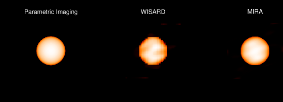
Figure 11: Three different images of Arcturus. On the left hand, image produced using a limb-darkening power law with parameter from Table 3. The two others images are obtained using two different softwares for regularized imaging. The right hand scale is derived using the Hipparcos parallax of $88.83\pm 0.53$ mas (Van Leeuwen 2007).

Model fitting confines the image to be within the range of a pre-defined model. This is a perfect tool to derive parameters of astronomical objects whose morphology is already known. However, it would not reveal any unexpected phenomenon, hence the need for less constraining image reconstruction.

The image is sought by minimizing a so-called cost function which is the sum of a regularization term plus data related terms. The data terms enforce the agreement of the model image with the different kind of measured data (power spectrum, phase closures, complex visibilities, etc). The interpolation of missing data is allowed by the regularization and by strict constraints such as the positivity (which plays the role of a floating support constraint) and normalization.

To validate this imaging process, we used two different reconstruction algorithms: Wisard and Mira. Wisard (Meimon 2005; Mugnier et al. 2008) stands for “Weak-phase Interferometric Sample Alternating Reconstruction Device”. Its approach consists in finding the image and the missing phase data jointly. This technique is called self-calibration in radio-interferometry (Cornwell & Wilkinson 1981) and has enabled reliable images to be reconstructed in situations of partial phase indetermination. The strength of Wisard is that it combines, within a Bayesian framework, a recently developed noise model approximation suited to optical interferometry data (Meimon et al. 2005), and an edge-preserving regularization (Mugnier et al. 2004) to deal with the sparsity of the data typical of optical interferometry.

Mira (Thiébaut et al. 2003) stands for “Multi-aperture Image Reconstruction Algorithm”. Compared to Wisard, Mira does not explicitly manage the missing Fourier phase information: all missing information is handled implicitly in the data related term. For instance, it is possible to reconstruct an image given only the Fourier modulus information (power spectrum data; Thiébaut 2007). A second difference – in these image reconstructions of Arcturus – lies in the chosen prior. Instead of an edge preserving regularization, we used for this reconstruction a quadratic regularization criterion. To that end, we computed a prior which is a parametric model image of a stellar surface (a quadratic limb darkening law). This method, similar to that used by Monnier et al. (2007b), has the particularity of requiring a rough model of the observed object. It will inject more information into the reconstruction, which in turn can give wrong results if the prior model is not right.

We shall note that both Wisard and Mira algorithms can use various types of priors (entropy, Tikhonov, etc). It is therefore possible to have both algorithms using the same prior. The phase management – explicit or implicit – will however be different.

The images reconstructed by Wisard and Mira are shown in Fig. 11. A third representation of Arcturus is also presented. It is an image reconstructed from the parameters derived by fitting a power law limb-darkening prescription on the data (values presented in Table 3). We tentatively call such type of image reconstruction “Parametric imaging”. Cuts of the brightness distributions are presented Fig. 12. The similarity of the reconstructions is quite striking considering that the 2 reconstruction methods (i.e. data-fidelity terms), as well as the priors, are different.

5.2 Discussion of image reconstruction

The left hand image of Fig. 11 shows a featureless limb-darkened star. It is not a surprise since the image is strictly constrained by the prescription. However, the important result is the good fit of the prescription on our data. When doing parametric imaging, the $\chi^{2}$ is a strong information to judge the reliability of the image reconstruction. In this case, a reduced $\chi^{2}$ of 1.9 for 2413 degrees of freedom is a good validation of the derived image.

When dealing with regularized imaging, it is more difficult to judge the reliability of an image reconstruction. This is because the quantity which is minimized is a sum of a regularization term and a data term (generally, the $\chi^{2}$). The minimum of this cost function is therefore dependent on the regularization term, and no process is known which could use this minimum to judge on the quality of the reconstruction. The $\chi^{2}$ is still of interest, but does only give a partial view on the reliability of the reconstructed image: a reduced $\chi^{2}$ close to one is important, but it is not a quantity by itself which will ensure the quality of the image reconstruction.

Ultimately, the quality of image reconstruction will be dependent on the choice of the regularization term. The closer to the object the regularization term brings us, the closer to the reality our image reconstruction will be. According to this philosophy, it is important to have a good estimation of the prior. We recommend for optical interferometrist to use an adjustable regularization term. Simultaneously or sequentially, a solution we propose consists in: (i) fit a parametric image which best describe the data, and (ii) find the image which best fit both the data and the parametric image. This technique was the one used with the Mira reconstruction software.

6 Conclusion

Figure 12: Intensity slices through the $x$ and $y$ axes of the three images of Arcturus presented in Fig. 11. The solid curve correspond to the parametric image, the dashed curves to the Wisard reconstruction, and the dotted curves to the Mira reconstruction. If we suppose the limb darkening prescription to be the correct brightness distribution of the object, we can derive the residual of the reconstruction obtained by the two imaging softwares: the rms error is around 5% for the Wisard prior (edge-preserving) and 2-3% for Mira (limb-darkening prior).

In this paper, we presented an Arcturus dataset of interesting quality. With the IOTA/IONIC interferometer, we measured fringe contrasts of less than a percent, with errors bars in average below that level. Using this data, we fitted several models and prescriptions. The closure phases were well fitted by point-symmetric prescriptions. No companion at less than one AU was detected with an upper limit on its contrast ratio of $8\times 10^{-4}$. The same modeling of the closure phases allowed the derivation of an upper limit on the heterogeneity of the photosphere: no hotspot with a brightness above $1.7\times 10^{-3}$ the total flux of the photosphere was detected.

We adjusted Marcs atmospheric models to the data. The derived Rosseland diameter equaled $21.05\pm 0.21$ mas, most of the error bar being induced by non-trivial wavelength calibration. With a reduced $\chi^{2}$ of 2, it is interesting to note that atmosphere models of regular K giants can now be challenged by interferometry at a very fundamental level, even though spectroscopic agreement is near-perfect. Interestingly, we noted (i) a slight inconsistency in the magnitude of the limb-darkening at short wavelength ($\lambda\approx 1.55\,\mu$m; see Fig. 9), and (ii) a slight chromatic effect present in the residual (lower panel of Fig. 7). This last results could hint the presence of a marginal ($\approx 0.5$%) water vapor emission outside the photosphere.

Finally, we imaged the photosphere using two different reconstruction algorithms (Wisard and Mira). Both produced realistic images, but highlight the difficulty to judge the reliability of regularized image reconstruction. Comparatively, we presented an image reconstructed from an ad-hoc prescription of a limb darkened stellar surface. The low number of free parameters, combined with a good fit to the data, hinted to us that the most realistic brightness distribution is in fact the one of a simple limb darkened disk.