Phase behavior of parallel hard cylinders

Abstract

We test the performance of a recently proposed fundamental measure density functional of aligned hard cylinders by calculating the phase diagram of a monodisperse fluid of these particles. We consider all possible liquid crystalline symmetries, namely nematic, smectic and columnar, as well as the crystalline phase. For this purpose we introduce a Gaussian parameterization of the density profile and use it to minimize numerically the functional. We also determine, from the analytic expression for the structure factor of the uniform fluid, the bifurcation points from the nematic to the smectic and columnar phases. The equation of state, as obtained from functional minimization, is compared to the available Monte Carlo simulation. The agreement is is very good, nearly perfect in the description of the inhomogeneous phases. The columnar phase is found to be metastable with respect to the smectic or crystal phases, its free energy though being very close to that of the stable phases. This result justifies the observation of a window of stability of the columnar phase in some simulations, which disappears as the size of the system increases. The only important deviation between theory and simulations shows up in the location of the nematic-smectic transition. This is the common drawback of any fundamental measure functional of describing the uniform phase just with the accuracy of scaled particle theory.

I Introduction

Monte Carlo simulations conducted on systems of hard anisotropic particles (spherocylinders being the most paradigmatic shape) showed that the purely entropic nature of hard core interactions is enough to explain the stability of different liquid-crystalline phases and phase transitions between them Frenkel (1987a, b); Frenkel et al. (1988). These phases, in decreasing order of symmetry, are known as isotropic (I), nematic (N), smectic-A (Sm), columnar (C) and crystal (K) —the isotropic and the crystal not being liquid crystalline phases properly speaking—, and some of their physical and chemical properties have been described in detail in Refs. de Gennes and Prost (1994); Chandrasekhar (1992). Later, Monte Carlo simulations were also employed to calculate the full phase diagram of fluids of freely-rotating hard spherocylinders Bolhuis and Frenkel (1997) and hard-cut spheres Veerman and Frenkel (1992), including non-uniform phases as the periodic one-dimensional (Sm), two-dimensional (C) and three-dimensional (K) phases.

Several density functional theories have been devised to determine the phase behavior of the hard sphere (HS) fluid. These theories can be grouped in two different sets. The first one, the weighted-density functionals, are constructed from the knowledge of the thermodynamical and structural properties of the uniform fluid Tarazona (1984, 1985); Curtin and Ashcroft (1985), while the second one, the fundamental measure functionals (FMF), initially introduced by Rosenfeld Rosenfeld (1989, 1990) and later improved for an adequate description of the HS freezing Rosenfeld et al. (1996, 1997); Tarazona and Rosenfeld (1997), are built on the geometry of the particles alone.

The extensions of these theories to hard anisotropic particles have not been as successful as they have been for HS. There are two reasons to explain this difficulty: The first one is related to the, as of today, still poor knowledge of the structural properties of fluids composed by anisotropic particles, and the second one is the inherent complexity in dealing with orientational degrees of freedom within density functional theory. This notwithstanding, some weighted-density functionals have been developed for the fluid of hard spherocylinders Poniewierski and Hołyst (1988); Somoza and Tarazona (1989) to study both the I-Sm and the N-Sm phase transitions as a function of the particle aspect ratio. These functionals were constructed as modifications of a reference HS weighted-density functionals, and their predictions, tested against Monte Carlo simulations, are reasonably good. They do not allow though to properly account for the C and K phases.

FMF are more appropriate to treat these phases as, by construction, they are more suitable to describe highly confined particles, such as they are in a solid. Unfortunately the fundamental measure formalism has little flexibility to apply it to arbitrary geometries. FMF have been obtained for parallelepipeds with restricted orientations of their principal axes Cuesta (1996); Cuesta and Martínez-Ratón (1997a, b), and very recently for cylinders also with a parallel alignment constraint Martínez-Ratón et al. (2008). For freely rotating anisotropic particles FMF have been obtained for needles, infinitely thin plates, and their mixtures Schmidt (2001); Brader et al. (2002); Esztermann and Schmidt (2004); Esztermann et al. (2006), but this time the price to pay is to eliminate at least one of the characteristic lengths of the particles. Besides, the numerical minimization of these functionals to obtain the equilibrium density profiles of non-uniform phases seems to be a very demanding task.

In this article we aim at testing the recently proposed FMF for parallel hard cylinders Martínez-Ratón et al. (2008) by comparing its predictions with Monte Carlo simulations reported in the literature Stroobants et al. (1987); Veerman and Frenkel (1991). We will consider all possible non-uniform phases, namely N, Sm, C and K and will depict the phase diagram the FMF predicts. There is an interesting aspect about this model that poses a particularly stringent test on the theory. In Ref. Stroobants et al. (1987) a window of stability of the C phase was reported whose existence the authors of Ref. Veerman and Frenkel (1991) could not completely settle, although their results pointed to its being a finite size effect because this window disappears —being preempted by a K— in simulations of very large systems. We will show that our FMF does indeed confirm this conclusion by showing that either the Sm or the K are always more stable than the C, although the difference in free energy is rather small —what justifies its observation in small systems. We will also compare the resulting equations of state for the N, Sm and K phases with those obtained from the Monte Carlo simulations of Ref. Veerman and Frenkel (1991) and conclude that the performance of our functional is almost perfect in the description of highly non-uniform phases, even improving on the free-volume description of the K phase.

II Fundamental measure density functional

In Martínez-Ratón et al. (2008) we obtained a fundamental-measure density functional for mixtures of parallel hard cylinders, so we will just gather here the formulae, specialized for the case of a one-component fluid. The functional is constructed out of the one for two-dimensional hard disk. There are two versions for the latter: Rosenfeld’s original version Rosenfeld (1990), and the version of Tarazona and Rosenfeld Tarazona and Rosenfeld (1997). The former has some important drawbacks, for instance, the low density limit of the functional is only approximate. That of Tarazona and Rosenfeld recovers the exact result in this limit. On the other hand, the former is easier to implement than the latter, because it is expressible in terms of one-particle-weighted densities, while that of Tarazona and Rosenfeld contains a two-particle-weighted density. Nevertheless both are amenable to numerical treatment and we will explore the results of both. So the formulae presented here will describe the implementation of the two versions for the functional of parallel hard cylinders.

Irrespective of the version we are using, the free-energy density functional can always be written

$$\beta\mathcal{F}[\rho]=\beta\mathcal{F}_{\rm id}[\rho]+\beta\mathcal{F}_{\rm ex}[\rho],$$ (1)

where $\beta$ is the inverse temperature in units of the Boltzmann constant,

$$\beta\mathcal{F}_{\rm id}[\rho]=\int d{\bf r}\int dz\,\rho({\bf r},z)\left[\ln\mathcal{V}\rho({\bf r},z)-1\right]$$ (2)

is the functional of the ideal gas ($\mathcal{V}$ is the thermal volume, irrelevant for the phase behavior), and $\beta\mathcal{F}_{\rm ex}[\rho]$ is the excess free energy due to interactions. We are using the notation ${\bf r}=(x,y)$ for vectors perpendicular to the cylinders axes. Fundamental-measure functionals are expressed in terms of an excess free-energy density $\Phi({\bf r},z)$, such that

$$\beta\mathcal{F}_{\rm ex}[\rho]=\int d{\bf r}\int dz\,\Phi({\bf r},z).$$ (3)

This free-energy density can be given as a function of a set of weighted densities. The whole set of them can be written in terms of the two densities

$$\rho_{0}({\bf r},z) = \frac{1}{2}\left[\rho({\bf r},z+L/2)+\rho({\bf r},z-L/2)\right],$$ (4)

$$\rho_{1}({\bf r},z) = \int_{z-L/2}^{z+L/2}\rho({\bf r},t)\,dt.$$ (5)

Common to both versions are the weighted densities

$$n_{0}({\bf r},z) = \frac{1}{2\pi R}\int\limits_{|{\bf R}|=R}\rho_{0}({\bf r}+{\bf R},z)\,d{\bf R},$$ (6)

$$n_{1}({\bf r},z) = \frac{1}{2\pi R}\int\limits_{|{\bf R}|=R}\rho_{1}({\bf r}+{\bf R},z)\,d{\bf R},$$ (7)

$$n_{2}({\bf r},z) = \int\limits_{|{\bf R}|\leq R}\rho_{0}({\bf r}+{\bf R},z)\,d{\bf R},$$ (8)

$$n_{3}({\bf r},z) = \int\limits_{|{\bf R}|\leq R}\rho_{1}({\bf r}+{\bf R},z)\,d{\bf R}.$$ (9)

For Rosenfeld’s original version Rosenfeld (1990) there are also two vector densities, namely

$${\bf v}_{1}({\bf r},z) = \frac{1}{2\pi R^{2}}\int\limits_{|{\bf R}|=R}\rho_{0}({\bf r}+{\bf R},z){\bf R}\,d{\bf R},$$ (10)

$${\bf v}_{2}({\bf r},z) = \frac{1}{2\pi R^{2}}\int\limits_{|{\bf R}|=R}\rho_{1}({\bf r}+{\bf R},z){\bf R}\,d{\bf R},$$ (11)

and the expression for the excess free-energy density is

$$\Phi_{\rm Ros}=-n_{0}\ln(1-n_{3})+\frac{n_{1}n_{2}+2\pi R^{2}(n_{0}n_{1}-{\bf v}_{1}\cdot{\bf v}_{2})}{1-n_{3}}+\pi R^{2}n_{2}\,\frac{n_{1}^{2}-{\bf v}_{2}^{2}}{(1-n_{3})^{2}}.$$ (12)

For Tarazona-Rosenfeld’s version Tarazona and Rosenfeld (1997) there are also two two-particle-weighted densities, namely

$$N_{1}({\bf r},z) = \int\limits_{|{\bf R}_{1}|=R_{1}}d{\bf R}_{1}\int\limits_{|{\bf R}_{2}|=R_{2}}d{\bf R}_{2}\,\left[\rho_{1}({\bf r}+{\bf R}_{1},z)\rho_{0}({\bf r}+{\bf R}_{2},z)+\rho_{0}({\bf r}+{\bf R}_{1},z)\rho_{1}({\bf r}+{\bf R}_{2},z)\right]$$ (13)

$$\times K\left(\frac{|{\bf R}_{1}-{\bf R}_{2}|}{2R}\right),$$

$$N_{2}({\bf r},z) = \int\limits_{|{\bf R}_{1}|=R_{1}}d{\bf R}_{1}\int\limits_{|{\bf R}_{2}|=R_{2}}d{\bf R}_{2}\,\rho_{1}({\bf r}+{\bf R}_{1},z)\rho_{1}({\bf r}+{\bf R}_{2},z)K\left(\frac{|{\bf R}_{1}-{\bf R}_{2}|}{2R}\right),$$ (14)

where

$$K(x)=\frac{x}{\pi}\sqrt{1-x^{2}}\sin^{-1}x,$$ (15)

and the expression for the excess free-energy density is

$$\Phi=-n_{0}\ln(1-n_{3})+\frac{n_{1}n_{2}+N_{1}}{1-n_{3}}+\frac{n_{2}N_{2}}{(1-n_{3})^{2}}.$$ (16)

III Phase behavior

The Euler-Lagrange equation

$$\frac{\delta\beta\mathcal{F}}{\delta\rho({\bf r},z)}=\beta\mu,$$ (17)

provides the equilibrium density for the system when there is no external field and the chemical potential is fixed to $\mu$ (equivalently, when the mean density is fixed to the value $\rho$ corresponding to that chemical potential). Expected phases are nematic (no spatial ordering), smectic (one-dimensional layering of particles), columnar (two-dimensional odering of liquid columns) and crystal (a combination of both orderings). These are the phases shown in the simulations of Veerman and Frenkel Veerman and Frenkel (1991). Quite as expected, columnar phase is a triangular ordering of columns and crystal phase is a piling up of such triangular lattices, i.e. what is commonly referred to as an AAA crystal (see Fig. 1).

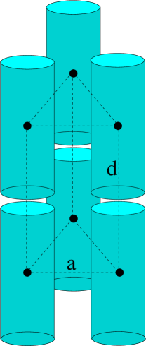
Figure 1: (Color online) Triangular (AAA) crystal. The lattice parameters $a$ and $d$ are shown in the figure.

A direct solution to (17) is numerically unfeasible so, as it is customary, we have resorted to a variational method. Thus, in order to account for all the above phases in our density functional description in a unified simple way, we have chosen the parametrization

$$\rho({\bf r}) = \rho V_{\rm{cell}}^{(D)}\chi_{\perp}({\bf r})\chi_{\parallel}(z),$$ (18)

where $\rho$ is the mean density (number of particles per unit volume) and

$$\chi_{\perp}({\bf r}) = \frac{\alpha_{\perp}}{\pi}\sum_{\bf k}\exp\left[-\alpha_{\perp}\left({\bf r}-{\bf R}_{\bf k}\right)^{2}\right],$$ (19)

$$\chi_{\parallel}(z) = \left(\frac{\alpha_{\parallel}}{\pi}\right)^{1/2}\sum_{k_{3}}\exp\left[-\alpha_{\parallel}(z-k_{3}d)^{2}\right].$$ (20)

The parameter $V_{\rm{cell}}^{(D)}$ is defined as the $D$-dimensional volume of the unit cell of the corresponding phase ($D=1$ smectic, $D=2$ columnar, $D=3$ crystal). Its values are

$$V^{(1)}_{\rm cell}=d,\qquad V^{(2)}_{\rm cell}=\sqrt{3}a^{2}/2,\qquad V^{(3)}_{\rm cell}=d\sqrt{3}a^{2}/2,$$ (21)

$d$ being the layer spacing along the Z direction and $a$ the lattice parameter of the triangular lattice on the XY plane (see Fig. 1). Finally, ${\bf R}_{\bf k}=k_{1}{\bf a}_{1}+k_{2}{\bf a}_{2}$ ($k_{1},k_{2}\in\mathbb{Z}$), with $\displaystyle{{\bf a}_{n}=\frac{a}{2}\left(\sqrt{3},(-1)^{n}\right)}$ the vectors defining the two-dimensional triangular lattice. In Appendix A we give explicit expressions for the weighted densities evaluated with the density profile (18).

When Eq. (17), using the parametrization (18), leads to a solution with $\alpha_{\parallel}=\alpha_{\perp}=0$, the equilibrium phase is a nematic; a smectic is the equilibrium phase if $\alpha_{\parallel}\neq 0$ and $\alpha_{\perp}=0$; it is a columnar if $\alpha_{\parallel}=0$ and $\alpha_{\perp}\neq 0$; and a crystal if both $\alpha_{\parallel}\neq 0$ and $\alpha_{\perp}\neq 0$. For the crystal phase $1-\rho V_{\rm{cell}}^{(3)}=\nu$ provides the fraction of vacancies.

III.1 Nematic phase

When $\alpha_{\parallel}=\alpha_{\perp}=0$ in (18), both (12) and (16) provide the same free-energy density, namely

$$\overline{\Phi}\equiv\frac{\beta Fv}{V}=\overline{\Phi}_{0}+\eta(\ln y+3y+y^{2}),$$ (22)

where $\overline{\Phi}_{0}=\eta\ln(\mathcal{V}/v)-\eta$, a linear term irrelevant for phase behavior, $\eta=\rho v$ is the packing fraction, $v=\pi R^{2}L$ is the volume of a cylinder, and $y=\eta/(1-\eta)$. This free-energy density is plotted in Fig. 2.

From (22) the equation of state is readily obtained as

$$\beta pv=y+3y^{2}+2y^{3}=\eta\,\frac{1+\eta}{(1-\eta)^{3}},$$ (23)

the same equation of state as that of parallel hard cubes Martínez-Ratón and Cuesta (1999).

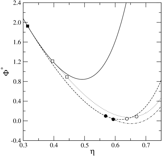
Figure 2: Free-energy densities $\Phi^{*}=\overline{\Phi}-\overline{\Phi}_{0}-a_{1}\eta-a_{2}$ (with $a_{1}=4.8463$ and $a_{2}=-2.0555$ chosen so as to amplify the differences between the different free-energy branches) vs. packing fraction $\eta$ for the nematic (solid line), smectic (dashed line), columnar (dotted line) and crystal (dash-dotted line) phases. The N-Sm bifurcation point is shown by a filled square. The nematic-columnar and smectic-columnar coexisting packing fractions are marked with open squares and open circles, respectively. The columnar phase is metastable and hence so are these two phase transitions. Before the smectic changes into a columnar the crystal becomes more stable. The smectic-crystal phase transition is marked with full circles.

The structure factor can also be obtained from the relationship $S(q,q_{z})=[1-\rho\hat{c}(q,q_{z})]^{-1}$, where $\hat{c}(q,q_{z})$ is the Fourier transform of the direct correlation function of the uniform fluid. Its expression was given in Ref. Martínez-Ratón et al. (2008) [cf. Eqs. (39)–(43) and Appendix B]. Specializing to the one-component fluid and taking into account that

$$\int d{\bf q}\,\delta(u-r) = 2\pi u\Psi_{0}(qu),$$ (24)

$$\int d{\bf q}\,\Theta(u-r) = \pi u^{2}\Psi_{1}(qu),$$ (25)

$$\int dq_{z}\,\Theta(u/2-|z|) = u\Psi_{2}(q_{z}u/2),$$ (26)

where ${\bf q}=(q_{x},q_{y})$, $q=|{\bf q}|$, $r=|{\bf r}|$, $\Psi_{0}(x)=J_{0}(x)$, $\psi_{1}(x)=2J_{1}(x)/x$ and $\Psi_{2}(x)=\sin x/x$, $J_{0}(x)$ and $J_{1}(x)$ being the zeroth and first order Bessel functions, respectively, we obtain, from the Tarazona-Rosenfeld functional (16), the following expression for the inverse structure factor

$$\begin{split}S(q,q_{z})^{-1}=&1+8y\Psi_{1}(2q^{*})\Psi_{2}(2q_{z}^{*})+4y^{2}\left[2\Psi_{0}(q^{*})\Psi_{1}(q^{*})\Psi_{2}(2q_{z}^{*})+\Psi_{1}(2q^{*})\Psi_{2}(q_{z}^{*})^{2}\right]\\ &+2y^{2}(1+2y)\left[2\Psi_{0}(q^{*})\Psi_{1}(q^{*})\Psi_{2}(q_{z}^{*})^{2}+\Psi_{1}(q^{*})^{2}\Psi_{2}(2q_{z}^{*})\right]\\ &+y^{2}(1+6y+6y^{2})\Psi_{1}(q^{*})^{2}\Psi_{2}(q_{z}^{*})^{2},\end{split}$$ (27)

where $q^{*}=Rq$ and $q_{z}^{*}=Lq_{z}/2$.

III.2 Smectic phase

When we set $\alpha_{\perp}=0$ in (18) and substitute this density profile into either (12) or (16), both yield the same expression

$$\Phi(z)=n_{0}(z)\left\{-\ln\left[1-n_{3}(z)\right]+\frac{3n_{3}(z)}{1-n_{3}(z)}+\frac{n_{3}(z)^{2}}{\left[1-n_{3}(z)\right]^{2}}\right\},$$ (28)

with

$$n_{0}(z) = \frac{1}{2}\left[\rho(z-L/2)+\rho(z+L/2)\right],$$ (29)

$$n_{3}(z) = \pi R^{2}\int_{z-L/2}^{z+L/2}dz^{\prime}\rho(z^{\prime}).$$ (30)

So both theories predict the same nematic-smectic transition.

Solving Eq. (17), a solution with $\alpha_{\parallel}\neq 0$ is found for every $\eta>\eta_{\rm N-Sm}\approx 0.31$ (also plotted in Fig. 2). The value of $\alpha_{\parallel}$ approaches zero as $\eta$ approaches this value from above. On the other hand, the free-energy density for this smectic phase is tangent to that of the nematic one (see Fig. 2), so the transition is continuous. This being so, we can obtain a more accurate value of $\eta_{\rm N-Sm}$ as the smallest $\eta$ at which the structure factor (27) diverges at some wave vector ${\bf q}={\bf 0}$, $q_{z}\neq 0$. Specializing (27) for such a wave vector we find

$$S(0,q_{z})^{-1}=1+2y(4+5y+2y^{2})\Psi_{2}(2q_{z}^{*})+y^{2}(9+14y+6y^{2})\Psi_{2}(q_{z}^{*})^{2}.$$ (31)

The smallest $\eta$ for which the right-hand side of (31) vanishes at a $q_{z}^{*}$ is $\eta_{\rm N-Sm}=0.3143$, and the value of $q_{z}^{*}$ at which it happens corresponds to a smectic period $d/L=\pi/q^{*}_{z}=1.3015$.

III.3 Columnar phase

At packing fraction $\eta^{*}_{\rm N-C}=0.4369$ the nematic loses stability against columnar ordering. This value is determined from the divergence of the structure factor (27) at a wave vector ${\bf q}\neq{\bf 0}$, $q_{z}=0$, which, for the Tarazona-Rosenfeld functional (16), is given by

$$S(q,0)^{-1}=1+4y(2+y)\Psi_{1}(2q^{*})+4y^{2}(3+2y)\Psi_{0}(q^{*})\Psi_{1}(q^{*})+y^{2}(3+10y+6y^{2})\Psi_{1}^{2}(q^{*}).$$ (32)

In this case, however, the columnar free energy is not tangent to the nematic one, so the transition is first order. We can determine the N-C coexistence by the usual double tangent construction. This yields the $\eta_{\rm N}=0.3957$ and $\eta_{\rm C}=0.4425$ as the coexisting packing fractions of the nematic and the columnar phases, respectively (see Fig. 2). At the latter, the lattice parameter is $a/R=2.4744$.

We can see here an important difference between this version of the functional and that based on Rosenfeld’s original approximation, Eq. (12). The latter leads to the following equation for the inverse structure factor

$$S(q,0)^{-1} = 1+2y(2+y)\left(\Psi_{0}^{2}(q^{*})-|\boldsymbol{\Psi}_{0}(q^{*})|^{2}\right)+2y(2+7y+4y^{2})\Psi_{0}(q^{*})\Psi_{1}(q^{*})$$ (33)

$$+y^{2}(3+10y+6y^{2})\Psi_{1}^{2}(q^{*}),$$

where the new complex vector $\displaystyle{\boldsymbol{\Psi}_{0}(q^{*})=iJ_{1}(q^{*}){\bf q}/q}$ has been introduced. The value of $\eta^{*}_{\rm N-C}$ which this approximation predicts is $\eta^{*}_{\rm N-C}=0.5599$. If we had to believe this value for the N-C bifurcation, the columnar free energy would be much too high to be consistent with the metastable columnar phase found in simulations Stroobants et al. (1987); Veerman and Frenkel (1991). For this reason, we have not pursued this version of the funcional anymore.

The columnar free energy is higher than the smectic one up to $\eta=0.6534$, where a first order Sm-C transition occurs, with coexisting packing fractions $\eta_{\rm Sm}=0.6382$ and $\eta_{\rm C}=0.6697$. However at these packing fractions the equilibrium phase is no more the smectic but the crystal, thus the columnar phase is always metastable, and in particular so are the N-C and the Sm-C transitions. All this can be easily visualized in Fig. 2.

III.4 Crystal phase

At packing fractions around $\eta\approx 0.58$ a solution to Eq. (17) with $\alpha_{\parallel}\neq 0$ and $\alpha_{\perp}\neq 0$ renders a free energy smaller than that of the, up to that point stable, smectic phase. The fluid undergoes a first order Sm-K transition with coexisting packing fractions $\eta_{\rm Sm}=0.5689$ and $\eta_{\rm K}=0.5936$. The lattice parameters of the coexisting crystal are $a/R=2.3102$ and $d/L=1.1419$. With these values the fraction of vacancies can be found to be just a mere 0.3%. The crystal is the only stable phase for $\eta>\eta_{\rm K}$ up to close packing (see Fig. 2).

IV Comparison with computer simulations

Numerical simulations for this fluid were carried out first by Stroobants et al. Stroobants et al. (1987) and later by Veerman and Frenkel Veerman and Frenkel (1991). The former, made with $900$ cylinders, showed the sequence of stable phases N-Sm-C-K. The latter confirmed this result but also made simulations with 1080 cylinders which showed that the columnar phase previously found appeared due to a finite size effect. Their conclusion was that the columnar phase is always metastable, but has a free energy very close to that of the smectic phase, so much that the boundary conditions may artificially render it more stable. Our previous calculations are fully consistent with this result, as Fig. 2 illustrates.

Besides this first qualitative agreement, we can also perform a more quantitative comparison with simulations by comparing the equations of state. This is done in Fig. 3. The simulation results are those obtained with the largest system size Veerman and Frenkel (1991). The figure shows that the agreement between the numerical values of the pressure is excellent for all stable phases. The values for the crystal phase are indistinguishable from the simulations, as it is also the location of the Sm-K transition.

The only important deviation between theory and simulations concerns the location of the N-Sm transition. While both, theory and simulation, predict that this transition is continuous, the theory predicts that it occurs at $\eta=0.3143$ while the simulations yield a value of $\eta=0.443$. This failure of the theory to predict the location of continuous transitions between low-density uniform and non-uniform phases is a fingerprint of FMT. For instance, the FMF of parallel hard cubes also predicts the same value of $\eta=0.3143$ for the transition between the fluid and the smectic, columnar and crystal phases (the later being the stable one) Cuesta and Martínez-Ratón (1997b); Martínez-Ratón (2004), while simulations provide a value of $\eta=0.49$ for the freezing of this fluid Jagla (1998); Groh and Mulder (2001). The reason for this drawback lies in the fact that, by construction, FMFs provide, in the uniform limit, the SPT equation of state —which for anisotropic bodies deviates from the exact result—, while at the same time the prediction for the nonuniform phases improves significantly due to the dimensional crossover properties of FMFs Tarazona (2002). This discrepancy in the accuracy with which the theory describes both type of phases leads to inaccurate predictions of the uniform-nonuniform phase transition points.

We end this section by comparing the EOS for the crystal phase given by the FMF and that obtained by a cell approximation for the fluid of parallel hard cylinders, which is derived in Appendix B. Figure 4 shows the results of both theories as well as the simulation results. As it can be seen, while the FMF results fit perfectly the simulation points, the cell approximation, although still a rather good description, underestimates the EOS. We can also see that, as expected, both theories converge at high densities, a known result which is a direct consequence of the dimensional crossover 3D$\to$0D of the FMF Rosenfeld et al. (1996, 1997).

Figure 3: Equations of state (reduced pressure vs. packing fraction) for all stable phases obtained from the fundamental measure functional for parallel hard cylinders. These phases are: nematic (for packing fractions up to the point indicated by a full rhombus), smectic (from that point up to the discontinuity) and crystal (from the discontinuity up to close packing). The open circles are the simulation results reported in Ref. Veerman and Frenkel (1991). Arrows mark the nematic-smectic and smectic-cystal phase transitions as obtained from those simulations. The two insets show the equations of state for the columnar metastable phase in the neighborhood of the nematic-columnar (left inset) and smectic-columnar (metastable) phase transitions. [Labels stand for nematic (N), smectic (Sm), columnar (C) and crystal (K).]

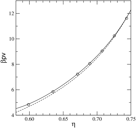
Figure 4: Comparison between the equation of state of the crystal phase as obtained from minimization of the functional (solid line), from the cell approximation (dashed line) and from simulations Veerman and Frenkel (1991).

V Conclusions

There are very few examples in the literature in which the same functional describes with accuracy all inhomogeneous phases of a liquid crystalline fluid. In this article we have applied a fundamental-measure functional recently proposed for mixtures of parallel hard cylinders Martínez-Ratón et al. (2008) to determine the phase behavior of the one-component fluid. As usual with fundamental-measure-based functionals, the results obtained for the uniform (nematic) fluid are those provided by scaled particle theory, and so the accuracy the functional provides for this phase is reasonably good but not perfect. As a consequence, the predicted nematic-smectic phase transition deviates significantly from the Monte Carlo simulations of Refs. Stroobants et al. (1987); Veerman and Frenkel (1991), although the order is correct. However, the accuracy with which the remaining stable phases, smectic and crystal, are obtained is excellent, the plots being indistinguishable from the simulation data, even for the smectic-crystal coexisting densities. Results for the equation of state of the crystal improve on those obtained by a cell approximation (which we have also reported in an appendix). Another correct prediction of the theory is that the columnar is only a metastable phase, but its free energy is sufficiently close to that of the stable phases so as to justify the observation of a window of stability of that phase in the oldest simulations Stroobants et al. (1987) made with the smallest system size, a window that disappears when the size in increased Veerman and Frenkel (1991). In summary, the proposed functional provides excellent results, very similar to those obtained by simulations, but obtained at a much cheaper price. They also made us confident that its version for mixture may provide very good results as well.

Appendix A Explicit expressions for the weighted densities

Insertion of the parametrization (18) into the expressions for the weighted densities (6)–(9) leads to the formulae

$$n_{0}({\bf r},z)=\rho V_{\rm{cell}}^{(D)}Q_{\phantom{i}\perp}^{(D)}({\bf r})P_{\phantom{i}\parallel}^{(D)}(z),$$ (34)

$$n_{1}({\bf r},z)=\rho V_{\rm{cell}}^{(D)}Q_{\phantom{i}\perp}^{(D)}({\bf r})H_{\phantom{i}\parallel}^{(D)}(z),$$ (35)

$$n_{2}({\bf r},z)=\rho V_{\rm{cell}}^{(D)}T_{\phantom{i}\perp}^{(D)}({\bf r})P_{\phantom{i}\parallel}^{(D)}(z),$$ (36)

$$n_{3}({\bf r},z)=\rho V_{\rm{cell}}^{(D)}T_{\phantom{i}\perp}^{(D)}({\bf r})H_{\phantom{i}\parallel}^{(D)}(z),$$ (37)

where $V_{\rm{cell}}^{(D)}$ is defined in Eq. (21). The functions are given in terms of

$$g_{\alpha}(x) = \left(\frac{\alpha}{\pi}\right)^{1/2}e^{-\alpha x^{2}},\qquad e_{\alpha}(x)=\frac{1}{2}\,{\rm erf}(\sqrt{\alpha}x),$$ (38)

${\rm erf}(x)$ being the standard error function. To be precise,

$$Q_{\phantom{i}\perp}^{(1)}({\bf r}) = 1,$$ (39)

$$Q_{\phantom{i}\perp}^{(2)}({\bf r}) = Q_{\phantom{i}\perp}^{(3)}({\bf r})=g_{\alpha_{\perp}}(R)\sum_{{\bf k}}g_{\alpha_{\perp}}(|{\bf r}-{\bf R}_{\bf k}|)I_{0}(2R\alpha_{\perp}|{\bf r}-{\bf R}_{\bf k}|),$$ (40)

where $I_{0}$ stands for the zeroth-order modified Bessel function of the first kind. The rest of the expressions are similar;

$$T_{\phantom{i}\perp}^{(1)}({\bf r}) = \pi R^{2},$$ (41)

$$T_{\phantom{i}\perp}^{(2)}({\bf r}) = T_{\phantom{i}\perp}^{(3)}({\bf r})=2\pi\sum_{\bf k}g_{\alpha_{\perp}}(|{\bf r}-{\bf R}_{\bf k}|)\int_{0}^{R}dt\,t\,g_{\alpha_{\perp}}(t)\,I_{0}(2t\alpha_{\perp}|{\bf r}-{\bf R}_{\bf k}|),$$ (42)

$$P_{\phantom{i}\parallel}^{(2)}(z) = 1,$$ (43)

$$P_{\phantom{i}\parallel}^{(1)}(z) = P_{\phantom{i}\parallel}^{(3)}(z)=\frac{1}{2}\sum_{k}[g_{\alpha_{\parallel}}(z-kd+L/2)+g_{\alpha_{\parallel}}(z-kd-L/2)],$$ (44)

$$H_{\phantom{i}\parallel}^{(2)}(z) = L,$$ (45)

$$H_{\phantom{i}\parallel}^{(1)}(z) = H_{\phantom{i}\parallel}^{(3)}(z)=\sum_{k}[e_{\alpha_{\parallel}}(z-kd+L/2)-e_{\alpha_{\parallel}}(z-kd-L/2)].$$ (46)

As for the two-particle weighted densities, after a lengthy calculation (see Ref. Martínez-Ratón et al. (2008) for some details) $N_{1}$ can be expressed as

$$N_{1}({\bf r},z)=2(\rho V_{\rm{cell}}^{(D)})^{2}P_{\phantom{i}\parallel}^{(D)}(z)H_{\phantom{i}\parallel}^{(D)}(z)J_{\phantom{i}\perp}^{(D)}({\bf r}),$$ (47)

with the functions $P_{\phantom{i}\parallel}^{(D)}$ and $H_{\phantom{i}\parallel}^{(D)}$ defined above. The radial contribution is

$$J_{\phantom{i}\perp}^{(1)}({\bf r}) = \pi R^{2},$$ (48)

$$J_{\phantom{i}\perp}^{(2)}({\bf r}) = J_{\phantom{i}\perp}^{(3)}({\bf r})=\left(\frac{\alpha_{\perp}}{\pi}\right)^{2}\!R^{2}e^{-2R^{2}\alpha_{\perp}}\!\!\sum_{{\bf k}_{1},{\bf k}_{2}}\!e^{-\alpha_{\perp}[({\bf r}-{\bf R}_{{\bf k}_{1}})^{2}+({\bf r}-{\bf R}_{{\bf k}_{2}})^{2}]}$$ (49)

$$\times\int_{0}^{\pi}dt\,t\sin t\,I_{0}[B_{{\bf k}_{1},{\bf k}_{2}}(t,{\bf r})],$$

where

$$B_{{\bf k}_{1},{\bf k}_{2}}(t,{\bf r})=2R\alpha_{\perp}\sqrt{\zeta_{{\bf k}_{1}}^{2}+\zeta_{{\bf k}_{2}}^{2}+2\zeta_{{\bf k}_{1}}\zeta_{{\bf k}_{2}}\cos(t+\psi_{{\bf k}_{2}}-\psi_{{\bf k}_{1}})},$$ (50)

denoting ${\bf r}-{\bf R}_{{\bf k}_{\nu}}=\zeta_{{\bf k}_{\nu}}(\cos\psi_{{\bf k}_{\nu}},\sin\psi_{{\bf k}_{\nu}})$, with $\nu=1,2$. Finally, $N_{2}$, is given by

$$N_{2}({\bf r},z)=[\rho V_{\rm{cell}}^{(D)}H_{\phantom{i}\parallel}^{(D)}(z)]^{2}J_{\phantom{i}\perp}^{(D)}({\bf r}).$$ (51)

Appendix B Cell approximation for the crystal phase of parallel hard cylinders

This section is devoted to obtain a cell approximation for the free energy per particle of the crystal phase of parallel hard cylinders. To this aim we first calculate the free volume available to one particle moving in an cell defined by the first nearest neighbours: a prism with hexagonal base composed by six triangular cells of period $a$ (see a sketch in Figure 5) and height equal to $2d$. Six hard disks (the cylinder sections) of radii $R$ are fixed at the vertexes of the hexagon while a seventh one is allowed to move within this cell, with the only constraint of not overlapping the other six disks (which of course do not overlap themselves). Simple geometric considerations lead, for the area accessible to the center of mass of the seventh disk, to the formula

$$A_{\rm{free}}=24R^{2}\left[\sqrt{3}x^{2}+\cos^{-1}x-x\sqrt{1-x^{2}}-\frac{\pi}{3}\right],$$ (52)

where $x=a/4R$. The free volume of this cell is simply $V_{\rm{free}}=2A_{\rm{free}}L(y-1)$ with $y=d/L$. If we fix the mean packing fraction of the crystal, the variables $x$ and $y$ are related through the equation $\eta=v/V^{(3)}_{\rm{cell}}$, where $v=\pi R^{2}L$ and $V^{(3)}_{\rm{cell}}$ is defined in (21), are the particle and cell volumes respectively. Thus $y=\pi/8\sqrt{3}\eta x^{2}$.

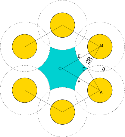
Figure 5: (Color online) Sketch of the triangular lattice of period $a$. The free region of area $A_{\rm{free}}$ within which one particle can move appears colored. One sixth of this area can be obtained substracting from the area of the triangle ABC those of the triangle ABD and of the sectors BED and ADF.

The cell theory approximates the free energy per particles as

$$\varphi=-\ln\left(\frac{V_{\rm{free}}}{\mathcal{V}}\right),$$ (53)

with $\mathcal{V}$ the thermal volume of the system, which in our case is

$$\varphi=\ln\left(\frac{\pi\mathcal{V}}{48v}\right)-\ln\left(\sqrt{3}x^{2}+\cos^{-1}x-x\sqrt{1-x^{2}}-\frac{\pi}{3}\right)-\ln\left(\frac{\pi}{8\sqrt{3}\eta x^{2}}-1\right).$$ (54)

Once the mean packing fraction is fixed the free-energy (54) must be minimized with respect to $x$ with the constraint $x\geq 1/2$ ($x=1/2$ represents the close packed limit), and then the pressure is obtained as $\displaystyle{\beta Pv=\eta^{2}\frac{\partial\varphi}{\partial\eta}}$, with the result

$$\beta Pv=\frac{\eta}{1-4x_{0}^{2}\eta/\eta_{\rm{cp}}},$$ (55)

$\eta_{\rm{cp}}=\pi/\sqrt{12}$ being the value of $\eta$ at close packing, and $x_{0}$ the solution to the equation

$$\frac{\eta_{cp}}{4\eta x^{2}}\left(\cos^{-1}x-\frac{\pi}{3}\right)+x\left(\sqrt{3}x-\sqrt{1-x^{2}}\right)=0.$$ (56)

References

- Frenkel (1987a) D. Frenkel, J. Phys. Chem. 91, 4912 (1987a).
- Frenkel (1987b) D. Frenkel, Molec. Phys. 60, 1 (1987b).
- Frenkel et al. (1988) D. Frenkel, H. N. W. Lekkerkerker, and A. Stroobants, Nature 332, 882 (1988).
- de Gennes and Prost (1994) P. G. de Gennes and J. Prost, The Physics of Liquid Crystals, 2nd ed. (Oxford University Press, Oxford, 1994).
- Chandrasekhar (1992) S. Chandrasekhar, Liquid Crystals (Cambridge University Press, Cambridge, 1992).
- Bolhuis and Frenkel (1997) P. Bolhuis and D. Frenkel, J. Chem. Phys. 106, 666 (1997).
- Veerman and Frenkel (1992) J. A. C. Veerman and D. Frenkel, Phys. Rev. A 45, 5632 (1992).
- Tarazona (1984) P. Tarazona, Molec. Phys. 52, 81 (1984).
- Tarazona (1985) P. Tarazona, Phys. Rev. A 31, 2672 (1985).
- Curtin and Ashcroft (1985) A. Curtin and N. W. Ashcroft, Phys. Rev. A 32, 2909 (1985).
- Rosenfeld (1989) Y. Rosenfeld, Phys. Rev. Lett. 63, 980 (1989).
- Rosenfeld (1990) Y. Rosenfeld, Phys. Rev. A 42, 5978 (1990).
- Rosenfeld et al. (1996) Y. Rosenfeld, M. Schmidt, H. Löwen, and P. Tarazona, J. Phys.: Condens. Matter 8, L577 (1996).
- Rosenfeld et al. (1997) Y. Rosenfeld, M. Schmidt, H. Löwen, and P. Tarazona, Phys. Rev. E 55, 4245 (1997).
- Tarazona and Rosenfeld (1997) P. Tarazona and Y. Rosenfeld, Phys. Rev. E 55, R4873 (1997).
- Poniewierski and Hołyst (1988) A. Poniewierski and R. Hołyst, Phys. Rev. Lett. 61, 2461 (1988).
- Somoza and Tarazona (1989) A. Somoza and P. Tarazona, J. Chem. Phys. 91, 517 (1989).
- Cuesta (1996) J. A. Cuesta, Phys. Rev. Lett. 76, 3742 (1996).
- Cuesta and Martínez-Ratón (1997a) J. A. Cuesta and Y. Martínez-Ratón, Phys. Rev. Lett. 78, 3681 (1997a).
- Cuesta and Martínez-Ratón (1997b) J. A. Cuesta and Y. Martínez-Ratón, J. Chem. Phys. 107, 6379 (1997b).
- Martínez-Ratón et al. (2008) Y. Martínez-Ratón, J. A. Capitán, and J. A. Cuesta (2008), preprint arXiv:0803.2033v1.
- Schmidt (2001) M. Schmidt, Phys. Rev. E 63, 010101(R) (2001).
- Brader et al. (2002) J. M. Brader, A. Esztermann, and M. Schmidt, Phys. Rev. E 66, 031401 (2002).
- Esztermann and Schmidt (2004) A. Esztermann and M. Schmidt, Phys. Rev. E 70, 022501 (2004).
- Esztermann et al. (2006) A. Esztermann, H. Reich, and M. Schmidt, Phys. Rev. E 73, 011409 (2006).
- Stroobants et al. (1987) A. Stroobants, H. N. W. Lekkerkerker, and D. Frenkel, Phys. Rev. A 36, 2929 (1987).
- Veerman and Frenkel (1991) J. A. C. Veerman and D. Frenkel, Phys. Rev. A 43, 4334 (1991).
- Martínez-Ratón and Cuesta (1999) Y. Martínez-Ratón and J. A. Cuesta, J. Chem. Phys. 111, 317 (1999).
- Martínez-Ratón (2004) Y. Martínez-Ratón, Phys. Rev. E 69, 061712 (2004).
- Jagla (1998) E. A. Jagla, Phys. Rev. E 58, 4701 (1998).
- Groh and Mulder (2001) B. Groh and B. Mulder, J. Chem. Phys. 114, 3653 (2001).
- Tarazona (2002) P. Tarazona, Physica A 306, 243 (2002).