CONTINUATION OF CONNECTING ORBITS IN 3D-ODES: (II) CYCLE-TO-CYCLE CONNECTIONS

1 Introduction

In a diversity of scientific fields bifurcation theory is used for the analysis of systems of ordinary differential equations (ODE’s) under parameter variation. Many interesting phenomena in ODE systems are linked to global bifurcations. Examples of such are overharvesting in ecological models with bistability properties (Bazykin, 1998; Antonovsky et al., 1990; Van Voorn et al., 2007), and the occurrence and disappearance of chaotic behaviour in such models. For example, it has been shown (see Kuznetsov et al., 2001 and Boer et al., 1999, 2001) that chaotic behaviour of the classical food chain models is associated with global bifurcations of point-to-point, point-to-cycle, and cycle-to-cycle connecting orbits.

In Part I of this paper (Doedel et al., 2007) we discussed heteroclinic connections between equilibria and cycles. Here we look at connections that link a cycle to itself (a homoclinic cycle-to-cycle connection, for which the cycle is necessarily saddle), or to another cycle (a heteroclinic cycle-to-cycle connection). Orbits homoclinic to the same hyperbolic cycle are classical objects of the Dynamical Systems Theory. It is known thanks to Poincare (1879), Birkhoff (1935), Smale (1963), Neimark (1967), and L.P. Shilnikov (1967) that a transversal intersection of the stable and unstable invariant manifolds of the cycle along such an orbit implies the existence of infinite number of saddle cycles nearby. Disappearance of the intersection via collision of two homoclinic orbits (homoclinic tangency) is an important global bifurcation for which the famous Hénon map turns to be a model Poincaré mapping (Gavrilov and Shilnikov, 1972; Palis and Takens, 1993, see also Kuznetsov, 2004).

Numerical methods for homoclinic orbits to equilibria have been devised by Doedel and Kernevez (1986, but see Doedel et al., 1997), who approximated homoclinic orbits by periodic orbits of large but fixed period. Beyn (1990) developed a direct numerical method for the computation of such connecting orbits and their associated parameter values, based on integral conditions and a truncated boundary value problem (BVP) with projection boundary conditions.

The continuation of homoclinic connections in auto (Doedel et al., 1997) improved with the development of HomCont by Champneys and Kuznetsov (1994) and Champneys et al. (1996). However, it is only suited for the continuation of bifurcations of homoclinic point-to-point connections and some heteroclinic point-to-point connections. A modification of this software was introduced by Demmel et al. (2000), that uses the continuation of invariant subspaces (CIS-algorithm) for the location and continuation of homoclinic point-to-point connections.

Dieci and Rebaza (2004) have also made significant progress recently, by developing methods to continue point-to-cycle and cycle-to-cycle connecting orbits based on another work by Beyn (1994). Their method employs a multiple shooting technique and requires the numerical solving for the monodromy matrices associated with the periodic cycles involved in the connection.

Our previous paper (Doedel et al., 2007) dealt with a method for the detection and continuation of point-to-cycle connections. Here this method is adapted for the continuation of homoclinic and heteroclinic cycle-to-cycle connections. The method is set up such that the homoclinic case is essentially a heteroclinic case where the same periodic orbit (but not the periodic solution) is doubled. In Section 2 we give a short overview of a BVP formulation to solve a heteroclinic cycle-to-cycle problem. In Section 3 it is shown how boundary conditions are implemented. In Section 4 we discuss starting strategies to obtain approximate connecting orbits using homotopy. In Section 5 the BVP is made suitable for numerical implementation.

Results are presented of the continuation of a homoclinic cycle-to-cycle connection in the standard three-level food chain model in Section 6. Boer et al. (1999) previously numerically obtained the two-parameter continuation curve of this connecting orbit using a shooting method, combined with the Poincaré map technique. In the previous part of this paper (Doedel et al., 2007) we reproduced the results for the structurally stable heteroclinic point-to-cycle connection of the same food chain model using the homotopy method. In this paper we discuss how the homoclinic cycle-to-cycle connection can be detected, and continued in parameter space using the homotopy method. Also, it is set up such that it can be used as well for a heteroclinic cycle-to-cycle connection.

2 Truncated BVPs with projection BCs

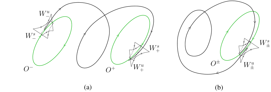
Figure 1: Cycle-to-cycle connecting orbits in ${\mathbb{R}}^{3}$: (a) heterolinic orbit, $O^{+}\neq O^{-}$; (b) homoclinic orbit, $O^{+}=O^{-}$.

Before presenting the BVP that describes a cycle-to-cycle connection, let us first set up some notation. Consider a general system of ODEs

$$\frac{du}{dt}=f(u,\alpha),$$ (1)

where $f:\mathbb{R}^{n}\times\mathbb{R}^{p}\to\mathbb{R}^{n}$ is sufficiently smooth, given that state variables $u\in\mathbb{R}^{n}$, and control parameters $\alpha\in\mathbb{R}^{p}$. Thus, the dimension of the state space is $n$ and the dimension of the parameter space is $p$. The (local) flow generated by (1) is denoted by $\varphi^{t}$. Whenever possible, we will not indicate explicitly the dependence of various objects on parameters.

We assume that both $O^{-}$ and $O^{+}$ are saddle limit cycles of (1). A solution $u(t)$ of (1) for fixed $\alpha$ defines a connecting orbit from $O^{-}$ to $O^{+}$ if

$$\lim_{t\to\pm\infty}{\rm dist}(u(t),O^{\pm})=0\;.$$ (2)

(Figure 1 depicts such a connecting orbit in the 3D-space.) Since $u(t+\tau)$ satisfies (1) and (2) for any phase shift $\tau$, an additional phase condition

$$\psi[u,\alpha]=0\;,$$ (3)

should be imposed to ensure uniqueness of the connecting solution. This condition will be specified later.

Table 1: List of notation used in the paper.

sym.	meaning
$x^{\pm}$	Periodic solution
$v^{\pm}$	Eigenfunction
$w^{\pm}$	Scaled adjoint eigenfunction
$u$	Connection
$\alpha$	Bifurcation parameters
$O^{+}$	Limit cycle where connection ends
$O^{-}$	Limit cycle where connection starts
$W^{s}_{+}$	Stable manifold of the cycle $O^{+}$
$W^{u}_{-}$	Unstable manifold of the cycle $O^{-}$
$\mu^{+}_{u}$	Unstable multiplier of the cycle $O^{+}$
$\mu^{-}_{s}$	Stable multiplier of the cycle $O^{-}$
$\mu^{-}_{u}$	Unstable multiplier of the cycle $O^{-}$
$\mu^{+}$	Adjoint multiplier $1/\mu^{+}_{u}$
$\mu^{-}$	Adjoint multiplier $1/\mu^{-}_{s}$
$\lambda^{\pm}$	$\ln(\mu^{\pm})$
$T^{\pm}$	Period of the cycle $O^{\pm}$
$T$	Connection time

For numerical approximations, the asymptotic conditions (2) are substituted by projection boundary conditions at the end-points of a large truncation interval $[\tau_{-},\tau_{+}]$, following Beyn (1994). It is prescribed that the points $u(\tau_{-})$ and $u(\tau_{+})$ belong to the linear subspaces, which are tangent to the unstable and stable invariant manifolds of $O^{-}$ and $O^{+}$, respectively.

Now, denote by $x^{\pm}(t)$ a periodic solution (with minimal period $T^{\pm}$) corresponding to $O^{\pm}$ and introduce the monodromy matrix

$$M^{\pm}=\left.D_{x}\varphi^{T^{\pm}}(x)\right|_{x=x^{\pm}(0)},$$

i.e. the linearization matrix of the $T^{\pm}$-shift along orbits of (1) at point $x_{0}^{\pm}=x^{\pm}(0)\in O^{\pm}$. Its eigenvalues are called Floquet multipliers, of which one (trivial) equals 1. Let $m_{s}^{+}=n_{s}^{+}+1$ be the dimension of the stable invariant manifold $W^{s}_{+}$ of the cycle $O^{+}$, where $n_{s}^{+}$ is the number of its multipliers satisfying

$$|\mu|<1.$$

Along the same line, $m_{u}^{-}=n_{u}^{-}+1$ is the dimension of the unstable invariant manifold $W^{u}_{-}$ of the cycle $O^{-}$, and $n_{u}^{-}$ is the number of its multipliers satisfying

$$|\mu|>1.$$

To have an isolated branch of cycle-to-cycle connecting orbits of (1) it is necessary that

$$p=n-m_{s}^{+}-m_{u}^{-}+2\;,$$ (4)

(see Beyn, 1994).

The projection boundary conditions in this case become

$$L^{\pm}(u(\tau_{\pm})-x^{\pm}(0))=0\;,$$ (5)

where $L^{-}$ is a $(n-m^{-}_{u})\times n$ matrix whose rows form a basis in the orthogonal complement to the linear subspace that is tangent to $W^{u}_{-}$ at $x^{-}(0)$. Similarly, $L^{+}$ is a $(n-m^{+}_{s})\times n$ matrix, such that its rows form a basis in the orthogonal complement to the linear subspace that is tangent to $W^{s}_{+}$ at $x^{+}(0)$.

The above construction also applies in the case when $O^{+}$ and $O^{-}$ coincide, i.e. we deal with a homoclinic orbit to a saddle limit cycle $O^{+}=O^{-}$. Note that, in general, the base points $x^{\pm}(0)\in O^{\pm}$ remain different (and so do the periodic solutions $x^{\pm}(t)$).

It can be proved that, generically, the truncated BVP composed of (1), a truncation of (3), and (5), has a unique solution branch $(\hat{u}(t,\hat{\alpha}),\hat{\alpha})$, provided that (1) has a connecting solution branch satisfying (3) and (4).

The truncation to the finite interval $[\tau_{-},\tau_{+}]$ causes an error. If $u$ is a generic connecting solution to (1) at parameter $\alpha$, then the following estimate holds in both cases:

$$\|(u|_{[\tau_{-},\tau_{+}]},\alpha)-(\hat{u},\hat{\alpha})\|\leq C{\rm e}^{-2\min(\mu_{-}|\tau_{-}|,\mu_{+}|\tau_{+}|)},$$ (6)

where $\|\cdot\|$ is an appropriate norm in the space $C^{1}([\tau_{-},\tau_{+}],{\mathbb{R}}^{n})\times{\mathbb{R}}^{p}$, $u|_{[\tau_{-},\tau_{+}]}$ is the restriction of $u$ to the truncation interval, and $\mu_{\pm}$ are determined by the eigenvalues of the monodromy matrices. For exact formulations, proofs, and references to earlier contributions, see Pampel (2001) and Dieci and Rebaza (2004, including Erratum).

3 New defining systems in $\mathbb{R}^{3}$

In this section we show how to implement the boundary conditions (5). We consider the case $n=3$ where $O^{-}$ and $O^{+}$ are saddle cycles and therefore always $m_{s}^{-}=m_{u}^{-}=2$ and $m_{s}^{+}=m_{u}^{+}=2$. Substitution in (4) gives the number of free parameters for the continuation $p=1$.

Note that the complete BVP will consist of 15 equations (2 saddle cycles, 2 eigendata for these cycles, and the connecting orbit) and 19 boundary conditions.

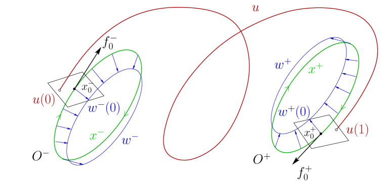
Figure 2: Ingredients of a BVP to approximate a heteroclinic connecting orbit. The homoclinic cycle-to-cycle connection is also approached as the heteroclinic case, where two saddle cycles coincide.

3.1 The cycle and eigenfunctions

To compute the saddle limit cycles $O^{-}$ and $O^{+}$ involved in the heteroclinic connection (see Figure 2) we need a BVP. The standard periodic BVP can be used

$$\left\{\begin{array}[]{rcl}\dot{x}^{\pm}-f(x^{\pm},\alpha)&=&0\;,\\ x^{\pm}(0)-x^{\pm}(T^{\pm})&=&0\;,\end{array}\right.$$ (7)

A unique solution of this BVP is determined by using an appropriate phase condition, which is actually a boundary condition for the truncated connecting solution, and which will be introduced below.

To set up the projection boundary condition for the truncated connecting solution $u$ near $O^{\pm}$, we also need a vector, say $w^{+}(0)$, that is orthogonal at $x^{+}(0)$ to the stable manifold $W^{s}_{+}$ of the saddle limit cycle $O^{+}$, as well another vector, say $w^{-}(0)$, that is orthogonal at $x^{-}(0)$ to the unstable manifold $W^{u}_{-}$ of the saddle limit cycle $O^{-}$ (see Figure 2). Each vector $w^{\pm}(0)$ can be obtained from an eigenfunction $w^{\pm}(t)$ of the adjoint variational problem associated with (7), corresponding to eigenvalue $\mu^{\pm}$. These eigenvalues satisfy

$$\mu^{+}=\frac{1}{\mu^{+}_{u}}\;,\;\mu^{-}=\frac{1}{\mu^{-}_{s}}\;,$$

where $\mu^{+}_{u}$ and $\mu^{-}_{s}$ are the multipliers of the monodromy matrix $M^{\pm}$ with

$$|\mu^{+}_{u}|>1\;,\;|\mu^{-}_{s}|<1\;.$$

The corresponding BVP is

$$\left\{\begin{array}[]{rcl}\dot{w}^{\pm}+f_{u}^{\rm T}(x^{\pm},\alpha)w^{\pm}&=&0\;,\\ w^{\pm}(T^{\pm})-\mu^{\pm}w^{\pm}(0)&=&0\;,\\ \langle w^{\pm}(0),w^{\pm}(0)\rangle-1&=&0\;,\end{array}\right.$$ (8)

where $x^{\pm}$ is the solution of (7). In our implementation the above BVP is replaced by an equivalent BVP

$$\left\{\begin{array}[]{rcl}\dot{w}^{\pm}+f_{u}^{\rm T}(x^{\pm},\alpha)w^{\pm}+\lambda^{\pm}w^{\pm}&=&0\;,\\ w^{\pm}(T^{\pm})-s^{\pm}w^{\pm}(0)&=&0\;,\\ \langle w^{\pm}(0),w^{\pm}(0)\rangle-1&=&0\;,\end{array}\right.$$ (9)

where $s^{\pm}={\rm sign\;}\mu^{\pm}$ and

$$\lambda^{\pm}=\ln|\mu^{\pm}|\;.$$

(See Appendix of Part I, Doedel et al., 2007).

In (9), the boundary conditions become periodic or anti-periodic, depending on the sign of the multiplier $\mu^{\pm}$, while the logarithm of its absolute value appears in the variational equation. This ensures high numerical robustness.

Given $w^{\pm}$ satisfies (9), the projection boundary conditions (5) become

$$\langle w^{\pm}(0),u(\tau_{\pm})-x^{\pm}(0)\rangle=0.$$ (10)

3.2 The connection

We use the following BVP for the connecting solution:

$$\left\{\begin{array}[]{rcl}\dot{u}-f(u,\alpha)&=&0\;,\\ \langle f(x^{\pm}(0),\alpha),u(\tau_{\pm})-x^{\pm}(0)\rangle&=&0\;.\end{array}\right.$$ (11)

For each cycle, a phase condition is needed to select a unique periodic solution among those which satisfy (7), i.e. to fix a base point $x_{0}^{\pm}=x^{\pm}(0)$ on the cycle $O^{\pm}$ (see Figure 2). For this we require the end-point of the connection to belong to a plane orthogonal to the vector $f(x^{+}(0),\alpha)$, and the starting point of the connection to belong to a plane orthogonal to the vector $f(x^{-}(0),\alpha)$. This allows the base points $x^{\pm}(0)$ to move freely and independently upon each other along the corresponding cycles $O^{\pm}$.

3.3 The complete BVP

The complete truncated BVP to be solved numerically consists of

$$\dot{x}^{\pm}-T^{\pm}f(x^{\pm},\alpha) =0,$$ (12a)

$$x^{\pm}(0)-x^{\pm}(1) =0\;,$$ (12b)

$$\dot{w}^{\pm}+T^{\pm}f_{u}^{\rm T}(x^{\pm},\alpha)w^{\pm}+\lambda^{\pm}w^{\pm} =0\;,$$ (12c)

$$w^{\pm}(1)-s^{\pm}w^{\pm}(0) =0,$$ (12d)

$$\langle w^{\pm}(0),w^{\pm}(0)\rangle-1 =0\;,$$ (12e)

$$\dot{u}-Tf(u,\alpha) =0\;,$$ (12f)

$$\langle f(x^{+}(0),\alpha),u(1)-x^{+}(0)\rangle =0\;,$$ (12g)

$$\langle f(x^{-}(0),\alpha),u(0)-x^{-}(0)\rangle =0\;,$$ (12h)

$$\langle w^{+}(0),u(1)-x^{+}(0)\rangle =0\;,$$ (12i)

$$\langle w^{-}(0),u(0)-x^{-}(0)\rangle =0\;,$$ (12j)

$$\|u(0)-x^{-}(0)\|^{2}-\varepsilon^{2} =0\;,$$ (12k)

where the last equation places the starting point $u(0)$ of the connection at a small fixed distance $\varepsilon>0$ from the base point $x^{-}(0)$. The time variable is scaled to the unit interval $[0,1]$, so that both the cycle periods $T^{\pm}$ and the connection time $T$ become parameters. Hence, besides a component of $\alpha$, there are five more parameters available for continuation: the connection time $T$, the cycle periods $T^{\pm}$, and the multipliers $\lambda^{\pm}$.

4 Starting strategies

The BVP described in the previous section are only usable when good initial starting data are available. Usually, such data are not present. Here we demonstrate how initial data can be generated through a series of successive continuations in auto, a method referred to as homotopy method, first introduced by Doedel, Friedman and Monteiro (1994) for point-to-point problems and extended to point-to-cycle problems in Part I of this paper.

4.1 Saddle cycles

The easiest way to obtain the limit saddle cycles $O^{\pm}$, first calculate a stable equilibrium using software like maple, matlab or mathematica. Then, using auto, continue this equilibrium up to an Andronov-Hopf bifurcation, where a stable limit cycle is generated. A continuation of this cycle can result in the detection of a fold bifurcation for the limit cycle. This will yield a saddle limit cycle.

4.2 Eigenfunctions

In order to obtain an initial starting point for the connecting orbit we require knowledge about the unstable manifold of the saddle limit cycle $O^{-}$. Also, we need the linearized adjoint “manifolds” to understand how the connecting orbit leaves $O^{-}$ and approaches $O^{+}$ (or the same cycle in the homoclinic case). For this, we look at the eigendata.

First consider the periodic BVP for $O^{-}$,

$$\left\{\begin{array}[]{rcl}\dot{x}^{-}-T^{-}f(x^{-},\alpha)&=&0\;,\\ x^{-}(0)-x^{-}(1)&=&0\;,\end{array}\right.$$ (13)

to which we add the standard integral phase condition

$$\int_{0}^{1}\langle\dot{x}^{-}_{old}(\tau),x^{-}(\tau)\rangle=0\;,$$ (14)

as well as a BVP similar to (8), namely

$$\left\{\begin{array}[]{rcl}\dot{v}-T^{-}f_{u}(x^{-},\alpha)v&=&0\;,\\ v(1)-\mu v(0)&=&0\;,\\ \langle v(0),v(0)\rangle-h&=&0\;.\end{array}\right.$$ (15)

In (14), $x^{-}_{old}$ is a reference periodic solution, e.g. from the preceding continuation step. The parameter $h$ in (15) is a homotopy parameter, that is set to zero initially. Then, (15) has a trivial solution

$$v(t)\equiv 0,\ \ h=0,$$

for any real $\mu$. This family of the trivial solutions parametrized by $\mu$ can be continued in auto using a BVP consisting of (13), (14), and (15) with free parameters $(\mu,h)$ and fixed $\alpha$. The unstable Floquet multiplier of $O^{-}$ then corresponds to a branch point at $\mu=\mu^{-}_{u}$ along this trivial solution family. auto can accurately locate such a point and switch to the nontrivial branch that emanates from it. This secondary family is continued in $(\mu,h)$ until the value $h=1$ is reached, which gives a normalized eigenfunction $v^{-}$ corresponding to the multiplier $\mu^{-}_{u}$. Note that in this continuation the value of $\mu$ remains constant, $\mu\equiv\mu^{-}_{u}$, up to numerical accuracy. For the initial starting point of the connection we use $v^{-}(0)$.

The same method is applicable to obtain the nontrivial scaled adjoint eigenfunctions $w^{\pm}$ of the saddle cycles. For this, the BVP

$$\left\{\begin{array}[]{rcl}\dot{w}^{\pm}+T^{\pm}f_{u}^{\rm T}(x^{\pm},\alpha)w^{\pm}+\lambda^{\pm}w^{\pm}&=&0\;,\\ w^{\pm}(1)-s^{\pm}w^{\pm}(0)&=&0\;,\\ \langle w^{\pm}(0),w^{\pm}(0)\rangle-h^{\pm}&=&0\;,\end{array}\right.$$ (16)

where $s^{\pm}={\rm sign}(\mu^{\pm})$, replaces (15). A branch point at $\lambda_{1}^{\pm}$ then corresponds to the adjoint multiplier $\sigma^{\pm}{\rm e}^{\lambda_{1}^{\pm}}$. After branch switching the desired eigendata can be obtained.

4.3 The connection

Time-integration of (1), in matlab for instance, can yield an initial connecting orbit, however, this only applies for non-stiff systems. Nevertheless, mostly when starting sufficiently close to the exact connecting orbit in parameter space the method of successive continuation (Doedel, Friedman and Monteiro, 1994) can be used to obtain an initial connecting orbit.

Let us introduce a BVP that is a modified version of (12)

$$\dot{x}^{\pm}-T^{\pm}f(x^{\pm},\alpha) =0\;,$$ (17a)

$$x^{\pm}(0)-x^{\pm}(1) =0\;,$$ (17b)

$$\Phi^{\pm}[x^{\pm}] =0\;,$$ (17c)

$$\dot{w}^{\pm}+T^{\pm}f_{u}^{\rm T}(x^{\pm},\alpha)w^{\pm}+\lambda^{\pm}w^{\pm} =0\;,$$ (17d)

$$w^{\pm}(1)-s^{\pm}w^{\pm}(0) =0\;,$$ (17e)

$$\langle w^{\pm}(0),w^{\pm}(0)\rangle-1 =0\;,$$ (17f)

$$\dot{u}-Tf(u,\alpha) =0,$$ (17g)

$$\langle f(x^{+}(0),\alpha),u(1)-x^{+}(0)\rangle-h_{11} =0\;,$$ (17h)

$$\langle f(x^{-}(0),\alpha),u(0)-x^{-}(0)\rangle-h_{12} =0\;,$$ (17i)

$$\langle w^{+}(0),u(1)-x^{+}(0)\rangle-h_{21} =0\;,$$ (17j)

$$\langle w^{-}(0),u(0)-x^{-}(0)\rangle-h_{22} =0\;,$$ (17k)

where each $\Phi^{\pm}$ in (17c) defines any phase condition fixing the base point $x^{\pm}(0)$ on the cycle $O^{\pm}$. An example of such a phase condition is

$$\Phi^{+}[x]=x_{j}(0)-a_{j}\;,$$

where $a_{j}$ is the $j$th-coordinate of the base point of $O^{+}$ at some given parameter values. Furthermore, $h_{jk}$, $j,k=1,2,$ in (17h)–(17k) are homotopy parameters.

For the approximate connecting orbit a small step $\varepsilon$ is made in the direction of the unstable eigenfunction $v^{-}$ of the cycle $O^{-}$:

$$u(\tau)=x^{-}(0)+\varepsilon v^{-}(0){\rm e}^{\mu^{-}_{u}T^{-}\tau},~{}~{}\tau\in[0,1]\;,$$ (18)

which provides an approximation to a solution of $\dot{u}=T^{-}f(u,\alpha)$ in the unstable manifold $W^{u}_{-}$ near $O^{-}$. After collection of the cycle-related data, eigendata and the time-integrated approximated orbit, a solution to the above BVP can be continued in $(T,h_{11})$ and $(T,h_{12})$ for fixed value of $\alpha$ in order to make $h_{11}=h_{12}=0$, while $u(1)$ is near the cycle $O^{+}$, so that $T$ becomes sufficiently large. In the next step, we then try to make $h_{21}=h_{22}=0$, after which a good approximate initial connecting orbit is obtained.

This solution is now used to activate one of the system parameters, say $\alpha_{1}$, and to continue a solution to the primary BVP (12). Then, if necessary after having improved the connection first by a continuation in $T$, continuation in $(\alpha_{1},T)$ can be done to detect limit points, using the standard fold-detection facilities of auto. Subsequently a fold curve can be continued in two parameters, say $(\alpha_{1},\alpha_{2})$, for fixed $T$ using the standard fold-following facilities in auto.

5 Implementation in AUTO

Our algorithms have been implemented in auto, which solves the boundary value problems using superconvergent orthogonal collocation with adaptive meshes. auto can compute paths of solutions to boundary value problems with integral constraints and non-separated boundary conditions:

$$\dot{U}(\tau)-F(U(\tau),\beta) =0\;,\;\;\tau\in[0,1],$$ (19a)

$$b(U(0),U(1),\beta) =0\;,$$ (19b)

$$\int^{1}_{0}q(U(\tau),\beta)d\tau =0\;,$$ (19c)

where

$$U(\cdot),F(\cdot,\cdot)\in{\mathbb{R}}^{n_{d}},~{}b(\cdot,\cdot)\in{\mathbb{R}}^{n_{bc}},~{}q(\cdot,\cdot)\in{\mathbb{R}}^{n_{ic}},$$

and

$$\beta\in{\mathbb{R}}^{n_{fp}},$$

as $n_{fp}$ free parameters $\beta$ are allowed to vary, where

$$n_{fp}=n_{bc}+n_{ic}-n_{d}+1\;.$$ (20)

The function $q$ can also depend on $F$, the derivative of $U$ with respect to pseudo-arclength, and on $\hat{U}$, the value of $U$ at the previously computed point on the solution family.

For our primary BVP problem (12) in three dimensions we have

$$n_{d}=15,~{}~{}n_{ic}=0,$$

and $n_{bc}=19$, so that any 5 free parameters are allowed to vary.

6 Example: food chain model

In this section we describe the performance of the BVP-method for the detection and continuation of a cycle-to-cycle connecting orbit in the standard food chain model, also used in Part I of this paper.

6.1 The model

The three-level food chain model from theoretical biology, based on the Rosenzweig-MacArthur (1963) prey-predator model, is given by the following equations

$$\left\{\begin{array}[]{rcl}\dot{x_{1}}&=&x_{1}(1-x_{1})-f_{1}(x_{1},x_{2})\;,\\ \dot{x_{2}}&=&f_{1}(x_{1},x_{2})-d_{1}x_{2}-f_{2}(x_{2},x_{3})\;,\\ \dot{x_{3}}&=&f_{2}(x_{2},x_{3})-d_{2}x_{3}\;,\end{array}\right.$$ (21)

with Holling Type-II functional responses

$$f_{1}(x_{1},x_{2})=\frac{a_{1}x_{1}x_{2}}{1+b_{1}x_{1}}\;$$

and

$$f_{2}(x_{2},x_{3})=\frac{a_{2}x_{2}x_{3}}{1+b_{2}x_{2}}\;.$$

This standard model has been studied by several authors, see e.g. Kuznetsov and Rinaldi (1996) and Kuznetsov et al. (2001) and references there.

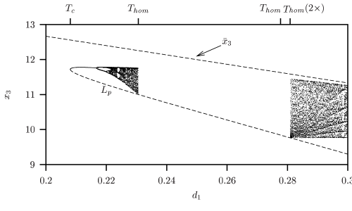
Figure 3: One-parameter bifurcation diagram for $d_{2}=0.0125$. The equilibrium is indicated as $\bar{x}_{3}$. The dashed line $L_{p}$ is the $x_{3}$-value of the local minimum of an unstable (saddle) limit cycle. At the point $T_{c}$ this limit cycle coincides with a stable limit cycle, of which the local minimum of $x_{3}$ is also shown. The stable limit cycle undergoes period doublings until chaos (the dense regions) is reached. The two dense regions are separated by a region where homoclinic cycle-to-cycle connections to the limit cycle $L_{p}$ exist. Both chaotic regions are bounded by a limit point of the homoclinic connection, indicated by $T_{hom}$. Observe that near the right chaotic region, between two limit points exist secondary connecting orbits to the cycle. One of these limit points coincides with the limit point of the primary connecting orbit that forms the boundary of the region of chaos (hence $T_{hom}$ twice); after Boer et al., 1999).

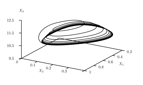
Figure 4: Phase plot of the homoclinic cycle-to-cycle connection.

The death rates $d_{1}$ and $d_{2}$ are often used as bifurcation parameters $\alpha_{1}$ and $\alpha_{2}$, respectively, with the other parameters set at $a_{1}=5$, $a_{2}=0.1$, $b_{1}=3$, and $b_{2}=2$. For these parameter values the model displays chaotic behaviour in a given parameter range of $d_{1}$ and $d_{2}$ (Hastings and Powell, 1991; Klebanoff and Hastings, 1994; McCann and Yodzis, 1995). The region of chaos can be found starting from a fold bifurcation at for instance $d_{1}\approx 0.2080452$, $d_{2}=0.0125$, where two limit cycles appear. The stable branch then undergoes a cascade of period-doublings (see Figure 3) until a region of chaos is reached.

Previous work by Boer et al. (1999, 2001) has shown that the parameter region where chaos occurs is intersected by homoclinic and heteroclinic global connections, and that this region is partly bounded by a homoclinic cycle-to-cycle connection, as shown in Figure 3. These results were obtained numerically using multiple shooting.

6.2 Homotopy

Using the technique discussed in this paper we first find the saddle limit cycle for $d_{1}=0.25$, $d_{2}=0.0125$. Since the cycle $O$ is both $O^{+}$ and $O^{-}$, we use the same initial base point

$$x^{\pm}(0)=(0.839783,0.125284,10.55288)$$

and the period $T^{\pm}=24.28225$. The logarithms of the nontrivial adjoint multipliers are

$$\lambda^{+}=-0.4399607\;,\;\lambda^{-}=6.414681\;.$$

The starting point of the initial “connecting” orbit is calculated by taking the base point $x^{-}(0)$ and multiplying the eigenfunction $v^{-}(0)$ by $\varepsilon=-0.001$

$$u(0)=x^{-}(0)+\varepsilon v^{-}(0)\;,$$ (22)

where

$$v^{-}(0)=(-1.5855\cdot 10^{-2},2.6935\cdot 10^{-2},-0.99951)\;,$$

and the resulting

$$u(0)=(0.839789,0.125274,10.55324)\;.$$

The connection time $T=503.168$.

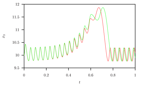
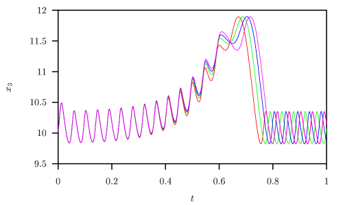
Figure 5: Profiles of the homoclinic cycle-to-cycle connections for $d_{2}=0.0125$. The left panel compares the two profiles of the connections for $d_{1}=0.2809078$, the right panel compares the four profiles for $d_{1}=0.27850$, which is between the limit points for the primary and secondary branches. The connection time $T$ is scaled to one.

To obtain a good initial connection we consider a BVP like (17), with 6 free parameters: $\mu^{\pm}$, $T^{\pm}$, $T$, and, in turn, one of the four homotopy parameters $h_{11},h_{12},h_{21},h_{22}$. The selected boundary conditions (17c) are

$$\Phi^{+}[x]=x_{2}^{-}(0)-0.125274\;,$$

and

$$\Phi^{-}[x]=x_{1}^{+}(0)-0.839789\;,$$

so, the first condition uses the $x_{2}$-coordinate of the initial base point selected on the cycle, while the second condition uses the $x_{1}$-coordinate of the initial base point. Observe, that this selection is somewhat arbitrary and that one can select other base point coordinates.

In the continuation we want $h_{11}=h_{12}=h_{21}=h_{22}=0$. However, there are several solutions, that correspond to connecting orbits with different numbers of excursions near the limit cycle, both at the starting and the end-part of the orbit. Observe that the success of the future continuation in $(d_{1},d_{2})$ seems to depend highly on the number of excursions near the cycle at the end-point of the connecting orbit. In the food chain model a decrease in $d_{2}$ is accompanied by a decrease in the numbers of excursions near the cycle at the end-point of the connection, like a wire around a reel. If this number is too low, a one-parameter continuation in $d_{1,2}$ will yield incorrect limit points. Also, two-parameter continuations in $(d_{1},d_{2})$ will most likely terminate at some point. Hence a starting orbit is selected with a sufficient number of excursions near the cycle at the end-point, with $T=454.04705$ and $\varepsilon^{2}=0.069414$.

6.3 Continuation

The continuation of the connecting orbit can be done in $d_{1,2}$ using the primary BVP (12). Equation (12k) ensures that the base points $x^{\pm}(0)\in O^{\pm}$ become different (and so do the periodic solutions $x^{\pm}(t)$).

First, however, using this BVP, the connection can be improved by increasing the connection time, for the same reason as mentioned above with regard to the number of excursions near the cycle at the end-point. The increase in $T$ results in an increase of the number of excursions near the cycle at the end-point of the connecting orbit. Then, the continuation in $d_{1,2},T$ results in the detection of four limit points, of which two are identical. Figure 3 shows a continuation in $d_{1}$ for fixed $d_{2}=0.0125$, that detects four limit points in one “run”. Observe that in this way not only the primary ($d_{1}=0.2809078$, twice, and $d_{1}=0.2305987$), but also the secondary ($d_{1}=0.2776909$) branch is detected. Figure 5 shows the profiles of the connecting orbits for $d_{2}=0.0125$. Observe that for the region of $0.2776909<d_{1}<0.2809078$ there are four different connecting orbits with the same connection time $T$ (see right panel).

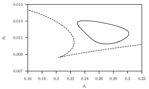
Figure 6: Two-parameter curves of the primary (left) and secondary (right) homoclinic cycle-to-cycle connections of the food chain model. Depicted is also the fold bifurcation curve of a limit cycle (dashed).

Using the standard fold-following facilities for BVPs in auto, both critical homoclinic orbits can be continued in two parameters ($d_{1},d_{2}$). Along these orbits the stable and unstable invariant manifold of the cycle are tangent. Starting from $d_{1}=0.2809078$ we continue the primary branch. The secondary branch is continued from $d_{1}=0.2776909$. Both curves are depicted in Figure 6.

7 Discussion

Our continuation method for cycle-to-cycle connections, using homotopies in a boundary value setting, is a modified method proposed in our previous paper for the continuation of point-to-cycle connections (Doedel et al., 2007). The results discussed here seem to be both robust and time-efficient. Detailed auto demos performing the computations described in Section 6 are freely downloadable from

www.bio.vu.nl/thb/research/project/globif.

Provided that the cycle has one simple unstable multiplier, the proposed method can be extended directly to homoclinic cycle-to-cycle connections in $n$-dimensional systems.

8 Acknowledgements

The research of the first author (GvV) is supported by the Dutch Organization for Scientific Research (NWO-CLS) grant no. 635,100,013.

References

- [Antonovsky et al., 1990] M.Ya. Antonovsky, R. A. Fleming, Yu. A. Kuznetsov, and W. C. Clark, [1990], “Forest–pest interaction dynamics: the simplest mathematical models,” Theor. Popul. Biol., 37, 343–367.
- [Bazykin, 1998] A. D. Bazykin, [1998], Nonlinear Dynamics of Interacting Populations. World Scientific, Singapore.
- [Beyn, 1990] W.-J. Beyn, [1990], “The numerical computation of connecting orbits in dynamical systems.,” IMA Journal of Numerical Analysis, 9, 379–405.
- [Beyn, 1994] W.-J. Beyn, [1994], “On well-posed problems for connecting orbits in dynamical systems”, In Chaotic Numerics (Geelong, 1993), volume 172 of Contemp. Math., 131–168. Amer. Math. Soc., Providence, RI.
- [Birkhoff, 1935] G. Birkhoff, [1935], “Nouvelles recherches sur les systèmes dynamiques,” Memoriae Pont. Acad. Sci. Novi. Lincaei, Ser. 3, 1, 85–216.
- [Boer et al., 1999] M. P. Boer, B. W. Kooi, and S. Kooijman, [1999], “Homoclinic and heteroclinic orbits in a tri-trophic food chain.,” Journal of Mathematical Biology, 39, 19–38.
- [Boer et al., 2001] M. P. Boer, B. W. Kooi, and S. Kooijman, [2001], “Multiple attractors and boundary crises in a tri-trophic food chain.,” Mathematical Biosciences, 169, 109–128.
- [Champneys and Kuznetsov, 1994] A. R. Champneys and Yu. A. Kuznetsov, [1994], “Numerical detection and continuation of codimension-two homoclinic bifurcations.,” International Journal of Bifurcation and Chaos, 4, 785–822.
- [Champneys et al., 1996] A. R. Champneys, Yu. A. Kuznetsov, and B. Sandstede, [1996], “A numerical toolbox for homoclinic bifurcation analysis.,” International Journal of Bifurcation and Chaos., 6(5), 867–887.
- [Demmel et al., 2000] J. W. Demmel, L. Diece, and M. J. Friedman, [2000], “Computing connecting orbits via an improved algorithm for continuing invariant subspaces.,” SIAM J. Sci. Comput., 22(1), 81–94.
- [Dieci and Rebaza, 2004a] L. Dieci and J. Rebaza, [2004], “Point-to-periodic and periodic-to-periodic connections.,” BIT Numerical Mathematics, 44, 41–62.
- [Dieci and Rebaza, 2004b] L. Dieci and J. Rebaza, [2004], “Erratum: “Point-to-periodic and periodic-to-periodic connections”,” BIT Numerical Mathematics, 44, 617–618.
- [Doedel et al., 1994] E. J. Doedel, M. J. Friedman, and A. C. Monteiro, [1994], “On locating connecting orbits,” Applied Mathematics and Computation, 65, 231–239.
- [Doedel et al., 1997] E. J. Doedel, A. R. Champneys, T. F. Fairgrieve, Yu. A. Kuznetsov, B. Sandstede, and X. Wang, [1997], “auto97: Continuation and bifurcation software for ordinary differential equations.”, Technical report, Concordia University, Montreal, Quebec, Canada.
- [Doedel et al., 2008] E. J. Doedel, B. W. Kooi, Yu. A. Kuznetsov, and G. A. K. Van Voorn, [2008], “Continuation of connecting orbits in 3D-ODEs: (I) Point-to-cycle connections,” International Journal of Bifurcation and Chaos. arXiv:0706.1688v1.
- [Gavrilov and Shilnikov, 1972] N.K. Gavrilov and L.P. Shilnikov, [1972], “On three-dimensional systems close to systems with a structurally unstable homoclinic curve: I,” Math. USSR-Sb., 17, 467–485.
- [Gavrilov and Shilnikov, 1973] N. K. Gavrilov and L. P. Shilnikov, [1973], “On three-dimensional systems close to systems with a structurally unstable homoclinic curve: II,” Math. USSR-Sb., 19, 139–156.
- [Hastings and Powell, 1991] A. Hastings and T. Powell, [1991], “Chaos in a three-species food chain.,” Ecology, 72, 896–903.
- [Klebanoff and Hastings, 1994] A. Klebanoff and A. Hastings, [1994], “Chaos in three species food chains.,” Journal of Mathematical Biology, 32, 427–451.
- [Kuznetsov and Rinaldi, 1996] Yu. A. Kuznetsov and S. Rinaldi, [1996], “Remarks on food chain dynamics.,” Mathematical Biosciences, 134, 1–33.
- [Kuznetsov et al., 2001] Yu. A. Kuznetsov, O. De Feo, and S. Rinaldi, [2001], “Belyakov homoclinic bifurcations in a tritrophic food chain model.,” SIAM Journal of Applied Mathematics, 62, 462–487.
- [Kuznetsov, 2004] Yu. A. Kuznetsov, [2004], Elements of Applied Bifurcation Theory., volume 112 of Applied Mathematical Sciences. Springer, 3th edition.
- [McCann and Yodzis, 1995] K. McCann and P. Yodzis, [1995], “Bifurcation structure of a three-species food chain model.,” Theoretical Population Biology, 48, 93–125.
- [Neimark, 1967] Ju. I. Neimark, [1967], “Motions close to doubly-asymptotic motion,” Soviet Math. Dokl., 8, 228–231.
- [Palis and Takens, 1993] J. Palis and F. Takens, [1993], Hyperbolicity and Sensitive Chaotic Dynamics at Homoclinic Bifurcations: Fractal Dimensions and Infinitely Many Attractors, volume 35 of Cambridge Studies in Advanced Mathematics. Cambridge University Press, Cambridge.
- [Pampel, 2001] T. Pampel, [2001], “Numerical approximation of connecting orbits with asymptotic rate,” Numerische Mathematik, 90, 309–348.
- [Poincaré, 1879] H. Poincaré, [1879], Sur les propriétés des fonctions définies par les équations aux différences partielles. Thèse. Gauthier-Villars, Paris.
- [Rosenzweig and MacArthur, 1963] M. L. Rosenzweig and R. H. MacArthur, [1963], “Graphical representation and stability conditions of predator-prey interactions.,” Am. Nat., 97, 209–223.
- [Shil’nikov, 1967] L. P. Shil’nikov, [1967], “On a Poincaré–Birkhoff problem,” Math. USSR-Sb., 3, 353–371.
- [Smale, 1963] S. Smale, [1963], “Diffeomorphisms with many periodic points”, In S. Carins, ed., Differential and Combinatorial Topology, 63–80. Princeton University Press, Princeton, NJ.
- [Van Voorn et al., 2007] G. A. K. Van Voorn, L. Hemerik, M. P. Boer, and B. W. Kooi, [2007], “Heteroclinic orbits indicate overexploitation in predator–prey systems with a strong Allee effect,” Math. Biosci., 209, 451–469.