Is a Dissipative Regime During Inflation in Agreement with Observations?

Abstract

We study the spectral index of curvature perturbations for inflationary models where the driving scalar field is coupled to a relativistic fluid through a friction term $\Gamma$. We find that only a very small friction term - $\Gamma\ll H$, with H being the Hubble parameter during inflation - is allowed by observations, otherwise curvature fluctuations are generated with a spectral index $n_{s}$ unacceptably red. These results are generic with respect to the inflationary potential and known dependence of the friction term on the scalar field and the energy density of the relativistic fluid. We compare our findings with previous investigations.

Introduction. The inflationary paradigm provides an explanation for the large-scale curvature fluctuations seen in the pattern of anisotropies of the cosmic microwave background and of the large scale structure books . Single scalar field inflationary models are successfull in matching observations if the effective mass of the inflaton - the second derivative of its potential $V(\phi)$ - is small compared to the energy scale at which inflation occurs komatsu . Primordial curvature perturbations are then generated with a spectrum close to scale invariance by the geometric amplification of zero point fluctuations. When several scalar fields conspire in driving inflation, beyond having isocurvature perturbation which are constrained by data if survived until decoupling between matter and radiation dunkley , their mutual interaction can drastically change the slope of the primordial spectrum of curvature perturbations during the exit from the Hubble radius KP .

Warm Inflation Warm inflation WI (see berera_review for a review) has been proposed as an alternative scenario where quantum fluctuations are not amplified just by geometry, but also by a production of radiation resulting from a decay of the inflaton occuring during the accelerated stage. In warm inflation the inflaton - taken in the literature and here as a standard scalar field - decays into radiation through a friction term in a phenomenological way, as in the old theory of reheating ASTW ; DL ; AFW . The value of the friction term $\Gamma$ was originally proposed to be much larger than the Hubble rate, but it may be also smaller BGB . Isocurvature perturbations are generic in this scenario and have been studied TB ; LF ; DFG , paying also attention to the post-inflationary evolution DFG . Both for large and small friction terms the spectrum of curvature perturbations is nearly scale invariant WI ; HMB ; BGB ; Hall-Peiris . Concerning the aspect of inflaton interactions, the case of warm inflation is therefore at odd with the argument above involving scalar fields in which the interactions of the inflaton have an important impact on the spectral index of curvature perturbations: although the key point of the warm inflationary scenario is the interaction of the inflaton with a relativistic fluid, no matter of how large this interaction is, the resulting spectrum of curvature perturbations is claimed to be nearly scale invariant in literature, and the strength of the friction term enter just in the small deviation from scale invariance also proportional to slow-roll parameters Hall-Peiris . In this paper we address this issue by the use of the standard theory of cosmological perturbations considering two different inflationary potential, i.e. a large field model:

$$V_{L}(\phi)=\frac{m^{2}}{2}\phi^{2}\,,$$ (1)

and as small field model, the SUSY breaking potential berera_PLB :

$$V_{S}(\phi)=\frac{1}{2}\mu^{2}\left[{\phi^{2}\log\frac{\phi^{2}}{\phi_{0}^{2}}+\phi_{0}^{2}-\phi^{2}}\right]\,.$$ (2)

For this last potential, we restrict ourselves to initial conditions for the inflaton close to the origin.

Background Eqs The simple equations of motion for the scalar field and the fluid energy-density $\rho_{F}$ we consider are the following:

$$\ddot{\phi}=-3H\dot{\phi}-\Gamma\dot{\phi}-\frac{dV(\phi)}{d\phi}$$ (3)

$$\dot{\rho}_{F}=-3H(1+\omega_{F})\rho_{F}+\Gamma\dot{\phi}^{2}\,,$$ (4)

where the dot denotes the derivative with respect to the cosmic time, $\omega_{F}=p_{F}/\rho_{F}$ is the fluid state parameter and the Friedmann equation is:

$$H^{2}=\frac{1}{3M_{\rm pl}^{2}}\left[\frac{{\dot{\phi}}^{2}}{2}+V(\phi)+\rho_{F}\right]\,,$$ (5)

with $M_{\rm pl}=1/\sqrt{8\pi G}$ as the reduced Planck mass. The coupling in Eqs. (3-4) admits a fully covariant description LF ; expl . The main idea of warm inflation is that dissipation of the inflaton in the perfect fluid elonges the slow-roll stage, as can be seen by:

$$(3H+\Gamma)\dot{\phi}\simeq-\frac{dV(\phi)}{d\phi}$$ (6)

and gently modifies it in a radiation dominated era through a continuous release of entropy. The fluid does not redshift as $1/a^{3(1+w_{F})}$ during inflation, but is also almost constant in time ($3H\rho_{F}(1+w_{F})\simeq\Gamma{\dot{\phi}}^{2}$). By taking as an example a massive inflaton and a decay rate constant in time, the elongation of the duration of inflation is encoded in the number of e-folds formula:

$$N=\frac{\phi_{\mathrm{i}}^{2}}{4M_{\mathrm{Pl}}^{2}}\Bigg{(}{1-\frac{\phi_{\mathrm{f}}^{2}}{\phi_{\mathrm{i}}^{2}}}\Bigg{)}+\frac{\Gamma\,\phi_{\mathrm{i}}}{\sqrt{6}\,M_{\mathrm{Pl}}\,m}\Bigg{(}1-\frac{\phi_{\mathrm{f}}}{\phi_{\mathrm{i}}}\Bigg{)}\,.$$ (7)

For future convenience we introduce the following adimensional parameter:

$$\gamma\equiv\frac{\Gamma(\phi,\rho_{F})}{3H}\mbox{,}$$ (8)

and the slow-roll parameters:

$$\epsilon\equiv-\frac{\dot{H}}{H^{2}}\mbox{,}\quad\eta_{\phi\phi}\equiv\frac{V_{\phi\phi}}{3H^{2}}\mbox{,}$$ (9)

where $V_{\phi\phi}=\frac{d^{2}V(\phi)}{d\phi^{2}}.$ We consider the most general case of $\Gamma=\Gamma(\phi,\rho_{F})$ HMB :

$$\Gamma=\Gamma_{0}\left({\frac{\phi}{\phi_{0}}}\right)^{b}\left({\frac{T}{M}}\right)^{c}\mbox{,}$$ (10)

where $M$ is a mass scale, $T=(\rho_{F}/\xi)^{1/4}$ with $\xi\equiv\frac{g_{*}}{30}\pi^{2}$, $g_{*}$ being the number of effective relativistic degrees of freedom.

Cosmological Perturbations in Warm Inflation For the analysis of scalar cosmological perturbations we follow Ref. DFG (the set of equations agrees with LF ; HMB ). In this work the full set of first-order equations were given in the uniform curvature gauge (UCG) for scalar metric perturbations:

$$ds^{2}=-(1+2\alpha)dt^{2}-a\beta_{,i}dtdx^{i}+a^{2}\delta_{ij}dx^{i}dx^{j}\,.$$ (11)

For the fluid the evolution of a redefinition of the 3-momentum scalar potential $\psi_{F}$ ($\delta T^{0}_{(F)i}\equiv\partial_{i}\psi_{F}$) DFG :

$$Q_{F}\equiv\frac{\psi_{F}}{\sqrt{\rho_{F}(1+w_{F})}}\,\mbox{,}$$ (12)

was considered in addition to the scalar field fluctuation $Q_{\phi}$. In the UCG the gauge-invariant scalar field and fluid fluctuations used for canonical quantization mukhanov ; lukash coincide with the field fluctuation $Q_{\phi}$ and $Q_{F}$. In the UCG the gauge-invariant comoving curvature perturbation is then simply written as the weighted sum of the field fluctuation $Q_{\phi}$ and the 3-momentum scalar potential of the fluid:

$$\mathcal{R}=H\frac{\dot{\phi}\,Q_{\phi}-\sqrt{\rho_{F}(1+w_{F})}\,Q_{F}}{{\dot{\phi}}^{2}+\rho_{F}(1+w_{F})}\mbox{.}$$ (13)

in full analogy with the more studied case of the two scalar field inflationary model system FB :

$$\mathcal{R}=H\frac{\dot{\phi}\,Q_{\phi}+\dot{\chi}\,Q_{\chi}}{{\dot{\phi}}^{2}+{\dot{\chi}}^{2}}\,\mbox{.}$$ (14)

Field and fluid fluctuations evolve in time according to DFG :

$${\ddot{Q}_{i}}+\left(3H\,\delta_{ij}+G_{ij}\right)\,{\dot{Q}_{j}}+{\Omega_{ij}}\,Q_{j}=0$$ (15)

where $(i\,,j)=(\phi\,,F)$ and $G_{ij}\,,\Omega_{ij}$ are given in Ref. DFG for $\Gamma={\rm const.}$ and generalized to $\Gamma=\Gamma(\phi,\rho_{F})$ in tesi ; talk . We have run numerical simulations following the system in Eq. (15) with initial conditions:

$$Q_{\phi|k}\simeq\frac{e^{-ik(\tau-\tau_{i})}}{a^{1+\frac{3}{2}\gamma}\sqrt{2k}}\mbox{,}\qquad Q_{F|k}\simeq\frac{e^{-i\omega_{F}^{1/2}k(\tau-\tau_{i})}}{a^{1+\frac{3}{2}(1+\omega_{F})}\sqrt[4]{4k^{2}\omega_{F}}}\mbox{,}$$ (16)

when $\tau$ stands for the conformal time coordinate (and $\tau_{i}$ is some initial time). These have been obtained analytically solving the evolution equations for $Q_{\phi|k}$ and $Q_{F|k}$ (shown in Ref. DFG ) with $k\gg aH$ and neglecting self-consistently cross terms in the time derivatives; the normalization factor has been evaluated in order to match the plane wave solution at early times. The power spectrum for the gauge-invariant comoving curvature perturbation

$$\mathcal{P}_{\mathcal{R}}=\frac{k^{3}|\mathcal{R}_{k}|^{2}}{2\pi^{2}}=A_{s}\left({\frac{k}{k_{*}}}\right)^{n_{S}-1}\mbox{,}$$ (17)

is evaluated numerically at the end of inflation. $k_{*}$ is a pivot scale, which is chosen to exit from the Hubble radius $51$ e-folds from the end of inflation; we consider a range of modes which spans three orders of magnitude centered around the pivot scale $k_{*}$.

Numerical Results The results for $n_{S}-1$ are presented in Table I and II for $w_{F}=1/3$, for the large and small field model, respectively. For the large field model only the case $\Gamma={\rm const.}$ ($b=c=0$ in Eq. (10)) is considered and one can see that already $\Gamma\sim m$ is inconsistent with observations, given the last constraints on the spectral index komatsu ; dunkley . For the small field model several possibilities allowed by Eq. (10) are considered with $M^{2}=\mu\phi_{0}/\sqrt{2}\,,g_{*}=100$: again $\gamma_{*}\gtrsim 0.01$ is inconsistent with observations.

Analytic argument for red spectra The numerical results can be easily understood analitically by considering the equation for $Q_{\phi}$ without potential and without coupling to $Q_{F}\,,\dot{Q}_{F}$ in a de Sitter space-time with $\Gamma$ constant in time. The equation for this massless fluctuation admits exact solutions in terms of the Hankel functions AS :

$$Q_{\phi|k}=\sqrt{\frac{\pi}{4H}}\frac{H_{\nu}^{(1)}(-k\eta)}{a^{3(1+\gamma)/2}}$$ (18)

with $\nu=\frac{3}{2}+\frac{\gamma}{2}$. This solution concides for $\gamma=0$ with the massless solution in de Sitter and has a solution constant in time for $-k\eta<<1$ with a spectral index $n_{S}-1=-3\gamma$. Following Stewart:1993bc , we provide also an expression for a quasi-De Sitter background in the simplest case of $\Gamma=\mathrm{const.}$:

$$n_{S}-1\simeq-3\,\gamma_{*}+\frac{2}{1+\gamma_{*}}\,\eta_{*}-6\frac{1+\gamma_{*}+\frac{1}{2}\gamma_{*}^{2}}{1+\gamma_{*}}\,\epsilon_{*}\mbox{,}$$ (19)

where $*$ stands for the time at which the pivot scale crosses the Hubble radius ($k_{*}=a_{*}\,H_{*}$). Eq. (19) agrees with the previous de Sitter expression for $\epsilon=\eta_{\phi\phi}=0$ and with the standard results of cold inflation Stewart:1993bc for $\gamma=0$. Our expression does not agree with the result quoted in literature for warm inflation in the quantum regime BGB ; Hall-Peiris :

$$n_{s}-1|_{\rm literature}=6\epsilon_{*}+2\eta_{*}+\gamma_{*}\left(8\epsilon_{*}-2\eta_{*}-2\beta_{*}\right)$$ (20)

where $\beta=M_{\rm pl}^{2}\Gamma_{\phi}V_{\phi}/(\Gamma V)$, but agrees very well with our numerical results diffs , as can be seen from Table I and II. Note how our result in Eq. (19) contains the dependence on $\Gamma$ linearly and not multiplied by the slow-roll parameters as in Eq. (20): the simple intuitive and correct argument to explain our result is the occurrence of $\Gamma$ in the equation of motion for the scalar field and its fluctuations not weighted by any slow-roll parameter.

$\frac{\Gamma_{0}}{m}$	$\frac{\phi_{\mathrm{i}}}{m_{\mathrm{Pl}}}$	$\frac{H_{\mathrm{i}}}{m}$	$\gamma_{*}$	$n_{S}-1$	$n_{S}-1$	$n_{S}-1$
				numerical	analytical	literature
0.01	3.34	6.83	0.00059	-0.0433	-0.0433	-0.0415
1	3.18	6.51	0.061	-0.219	-0.223	-0.364
8	2.28	4.67	0.71	-2.17	-2.21	0.00965

Table 1: Numerical and analytical spectral indexes in case of quadratic potential and $\Gamma=\mathrm{const.}$; the i subscript stands for initial and $*$ stands for the time at which the pivot scale crosses the Hubble radius ($k_{*}=a_{*}\,H_{*}$).

$\frac{\Gamma_{0}}{\mu}$	$b$	$c$	$\frac{\phi_{i}}{\phi_{0}}$	$\frac{H_{\mathrm{i}}}{\mu}$	$\gamma_{*}$	$n_{S}-1$	$n_{S}-1$	$n_{S}-1$
						numerical	analytical	literature
0.01	1	0	0.37	7.87	0.00022	-0.0398	-0.403	-0.0395
1	1	0	0.39	7.67	0.023	-0.109	-0.111	-0.0268
8	1	0	0.49	6.66	0.28	-0.854	-0.880	0.133
0.01	2	0	0.37	7.87	0.00010	- 0.0388	-0.0399	-0.0395
1	2	0	0.38	7.77	0.011	-0.0713	-0.0734	-0.0284
8	2	0	0.46	6.99	0.14	-0.461	-0.471	0.120
0.01	1	-1	0.38	7.77	0.0086	-0.0603	-0.0658	-0.347
0.1	1	-1	0.40	7.57	0.059	-0.201	-0.219	-0.00544
1	1	-1	0.59	5.46	0.83	-2.48	-2.56	0.591
0.01	2	-1	0.37	7.87	0.0047	-0.0474	-0.0539	-0.0346
0.1	2	-1	0.38	7.67	0.032	-0.135	-0.138	-0.00457
1	2	-1	0.56	5.81	0.50	-1.54	-1.57	0.644

Table 2: Numerical and analytical spectral indexes in case of small field model; the i subscript stands for initial and $*$ stands for the time at which the pivot scale crosses the Hubble radius ($k_{*}=a_{*}\,H_{*}$).

Explanation of the Discrepance A difference between our study and Ref. (HMB ) in the treatment of perturbations when they are in the sub-Hubble regime. Our treatment is the standard one which takes into account metric fluctuations self-consistently and which is used for any computation in a universe dominated by two scalar fields or fluids. Ref. HMB uses in this regime a Langevin equation for the field fluctuations in rigid space-time driven by a thermal bath claiming that fluctuations are scale invariant at freeze-out, i.e. at $k=a\,\sqrt{\Gamma H}$. Fig. (1) shows how the spectrum of curvature perturbations when evolved according to the system in Eq. (15) with initial conditions (16) is already red tilted at the freeze-out scale and far from scale invariance. We therefore conclude that the Langevin approximation used for sub-Hubble scales in HMB does not agree with the standard theory of cosmological perturbations.

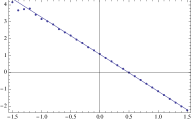
(a)  Large field model, with $\Gamma=8\,m$.

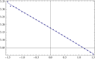
(b)  Small field model, with $\Gamma_{0}=1\,\mu$, $b=1$, $c=0$.

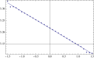
(c)  Small field model, with $\Gamma_{0}=1\,\mu$, $b=2$, $c=0$.

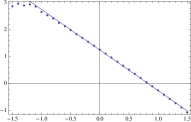
(d)  Small field model, with $\Gamma_{0}=1\,\mu$, $b=2$, $c=-1$.

Figure 1: Logarithm of the curvature perturbations power spectra vs $\log_{10}(k/k_{*})$. The dots are the spectra of curvature perturbations numerically evaluated at the freeze-out scale $k_{*}=a_{*}\sqrt{\Gamma_{*}H_{*}}$ in four case, one for the large field case and three for the small field case. The solid lines are the predictions for curvature perturbations based on Eq. (19). Note how the spectra are far from being scale invariant, which is the key prediction of Ref. HMB , and almost identical to their long-wavelength spectra.

Conclusions Warm inflation is an alternative to the pure geometric amplification in producing a nearly scale-invariant spectrum of curvature perturbations. It was argued YL that it is difficult to realize a strong dissipative regime described by Eqs. (3-5) from quantum field theory at finite temperature. In this paper we have shown a standard treatment of cosmological perturbations for the background system in Eqs. (3-5) leads to a spectrum of curvature perturbations which agrees with observations only when the dissipation is weak, starting from quantum initial fluctuations. It is not clear if the linear dependence of the spectral index of curvature perturbations on $\gamma$ found here may change by starting from thermal initial conditions, rather than from quantum ones, since quantum fluctuations are present anyway. It is however interesting that an introduction of a coupling along the lines of Eqs. (3-5) may bring cold inflationary models predicting a blue spectrum back in agreement with current observations.

- (1)
- (2) For a book review, see, e. g., E. W. Kolb and M. S. Turner, The Early Universe (Addison-Wesley, Redwood City, California, 1990); A. D. Linde, Particle Physics and Inflationary Cosmology (Harwood, Chur, Switzerland, 1990); A. R. Liddle and D. H. Lyth, Cosmological Inflation and Large Scale Structure (Cambridge, UK: Univ. Pr., 2000)
- (3) E. Komatsu et al., “Five-Year Wilkinson Microwave Anisotropy Probe (WMAP) Observations: Cosmological Interpretation,” arXiv:0803.0547 [astro-ph].
- (4) J. Dunkley et al. “Five-Year Wilkinson Microwave Anisotropy Probe (WMAP) Observations: Likelihoods and Parameters from the WMAP data,” arXiv:0803.0586 [astro-ph].
- (5) L. Kofman and D. Pogosyan, Phys. Lett. B 214 (1988) 508.
- (6) A. Berera, Phys. Rev. Lett. 75 (1995) 3218, A. Berera, Li-Zhi Fang, Phys. Rev. Lett. 74 (1995) 1912, A. Berera, Phys. Rev. D 55 3346 (1997); A. Berera, Nucl. Phys. 585, 666 (2000).
- (7) A. Berera, Grav. Cosmol. 11 (2005) 51
- (8) A. Albrecht, P. J. Steinhardt, M. S. Turner and F. Wilczek, Phys. Rev. Lett. 48 (1982) 1437.
- (9) A. Dolgov and A. D. Linde, Phys.Lett. 116B 329 (1982).
- (10) L. Abbott, E. Farhi and M. Wise, Phys.Lett. 117B 29 (1982).
- (11) M. Bastero-Gil and A. Berera, Phys. Rev. D 76 (2007) 043515
- (12) A. N. Taylor and A. Berera, Phys. Rev. D 62 (2004) 083517
- (13) W. Lee and L. Z. Fang, Phys. Rev. D 69 (2004) 023514
- (14) F. Di Marco, F. Finelli and A. Gruppuso, Phys. Rev. D 76, 043530 (2007).
- (15) L. M. H. Hall, I. G. Moss and A. Berera, Phys. Rev. D 69, 083525 (2004).
- (16) L. M. H. Hall and H. V. Peiris, JCAP 0801:027 (2008).
- (17) L. M. H. Hall, I. G. Moss and A. Berera, Phys. Lett. B 589, 1 (2004)
- (18) In covariant form the conservation equation for the fluid are written as , with being a normalized time-like vector.
- (19) V. N. Lukash, Sov. Phys. JETP 52 807 (1980).
- (20) V. F. Mukhanov, JETP Lett. 41, 493 (1985); Sov. Phys. JETP 68 1297 (1988).
- (21) F. Finelli and R. H. Brandenberger, Phys. Rev. D 62 (2000) 083502
- (22) A. Cerioni, Perturbazioni cosmologiche in un modello di inflazione con un campo scalare accoppiato ad un fluido perfetto, Tesi di Laurea Specialistica in Fisica, October 2007, Universitá degli Studi di Bologna (unpublished).
- (23) F. Finelli, Is a Dissipative Regime for the Inflaton in Agreement with Observations?, talk given at Rencontres de Moriond, La Thuile, Italy, March 16th, 2008.
- (24) M. Abramowitz and I. A. Stegun, Handbook of Mathematical Functions with Formulas, Graphs, and Mathematical Tables, 1964 New York, USA
- (25) E. D. Stewart and D. H. Lyth, Phys. Lett. B 302 (1993) 171
- (26) The percent difference between the numerical result and our analytic expression in Eq. (19) can be due to a) the way we approximate in closing the dynamics of in one single equation during inflation and/or b) the presence of isocurvature modes feeding the curvature perturbation and modifying slightly its spectral index during and after inflation and/or c) the deviations from when relevant.
- (27) J. Yokoyama and A. D. Linde, Phys. Rev. D 60 (1999) 083509