The Origins and Physical Properties of the Complex of Local Interstellar Clouds

Abstract

The Complex of Local Interstellar Clouds (CLIC) is a relatively tight grouping of low density, warm, partially ionized clouds within about 15 pc of the Solar System. The Local Interstellar Cloud (LIC) is the cloud observed on most lines of sight and may be the cloud that immediately surrounds our Solar System, the properties of which set the outer boundary conditions of the heliosphere. Using absorption line data toward nearby stars, in situ observations of inflowing interstellar gas from spacecraft in the Solar System, and theoretical modeling of the interstellar radiation field and radiative transfer, we can deduce many characteristics of the LIC. We find that the LIC is partially ionized with modest electron density, $n_{e}\approx 0.07$ cm^-3. The combination of its temperature and ionization favor photoionization/thermal equilibrium over a non-equilibrium cooling cloud picture. The abundances in the LIC suggest moderate dust destruction for silicate dust but complete destruction of carbonaceous grains. An origin for the LIC as a density enhancement in the ambient medium that has been overrun by a shock seems likely, while its velocity away from the Sco-Cen association points to a possible connection to that region and the Loop I bubble.

1 Introduction

The interstellar medium (ISM) that surrounds the Solar System impinges on the outflowing Solar wind creating the heliosphere. The particular characteristics of that circumheliospheric interstellar medium (CHISM), such as its density, ionization, temperature and magnetic field, determine in detail the interaction of the gas with the solar wind. Thus understanding the nature of the heliosphere requires knowledge of the state of the CHISM while at the same time interpretation of some of the in situ observations relevant to discerning the nature of the CHISM demands an understanding of the heliosphere.

It has long been assumed, because it appears on so many lines of sight, that the velocity component (or cloud) identified as the Local Interstellar Cloud (LIC) surrounds the heliosphere. Recently Redfield and Linsky (2008) have analyzed many lines of sight toward nearby stars and identified 15 distinct velocity vectors, which are attributed to coherent clouds in the local ISM. The LIC component, found in by far the most lines of sight, was found to have an associated temperature of $T=7500\pm 1300$ K. Redfield and Linsky (2008) claim that the heliosphere is located in a transition zone between the LIC and G cloud based on the fact that the temperature and velocity of the gas are intermediate between those found for the LIC and G cloud components. We believe that this is somewhat speculative as yet since the temperature of the inflowing gas is within the error bars on the LIC while falling outside of the error bars for the G cloud value. The inflowing gas velocity does appear to be somewhat discrepant ($2-3$ km s^-1) with their LIC vector, but that may be due to some weak disturbance in the cloud. Much of what we discuss does not depend specifically on whether the heliosphere is within the LIC as long as their properties are not very different, which appears to be the case. The primary assumption that we make related to this is that the portion of the line of sight between the Solar System and the star $\epsilon$ CMa that traverses the LIC can be treated as passing through a cloud that is in thermal and photoionization equilibrium.

2 The Physical Characteristics of the Complex of Local Interstellar Clouds

2.1 Primary Observational Evidence

The complex of local interstellar clouds, of which the Local Interstellar Cloud (LIC) that surrounds the Solar System is one member, are nearby, low density and partially ionized patches of gas that are surrounded by much lower density and (probably) hot ISM, the Local Bubble. We have the most information about the LIC since most sight lines to nearby stars pass through it, but the LIC is not extremely different from other clouds within the CLIC (see Redfield and Linsky, 2008, also Redfield, this volume).

Among the information on the LIC that we need to understand its origins are:

• ionization – is the LIC gas in photoionization equilibrium or not?,

• abundances – important for evaluating ionization corrections, radiative cooling rate and as evidence for dust destruction or enrichment,

• temperature/density/pressure – where does the LIC fit into typical ISM phase picture? Is the LIC in thermal equilibrium?,

• velocity – can provide hints as to the dynamics, history and past environment of the LIC,

• magnetic field – both the strength and orientation affect the size and shape of the heliosphere. The field also provides pressure support for the cloud and can play an important role in determining the nature of the cloud boundary.

Some of this information is relatively directly measureable, e.g. the temperature of the cloud at the Solar System via He⁰ temperature observations (Witte, 2004), but most require some modeling to infer their values.

Evidence on the nature of the LIC comes from a wide variety of sources. There is a large database of ion absorption lines toward nearby stars wherein particular velocity components have been identified as being due to the LIC (see Redfield and Linsky, 2008, and references therein). This has been accomplished by finding a consistent velocity vector for the cloud given the observed projections for many lines of sight.

Among the important ions for which column densities have been observed for the LIC are: Mg ii, Mg i, C ii^∗, S ii, and Fe ii. The importance of these ions lies in the constraints they place on the physical state of the cloud. As we discuss below, with Mg ii and Mg i we can determine the electron density. With the addition of C ii^∗, Si ii and Fe ii we gain information on the elemental abundances of dust components. These along with S ii provide necessary information on the total cooling within the cloud, which is primarily due to forbidden line emission. In order to understand the ionization and thermal properties of the cloud it is necessary to have data on these column densities and data on more ions will generally help to constrain the models better.

The most direct evidence on the state of the CHISM comes from observations of neutral He. Because of its small cross section for charge transfer reactions, He⁰ is believed to sail through the bowshock, heliopause and termination shock essentially unaffected. As a result the measurements of He⁰ density and temperature, $n(\mathrm{He}^{0})=0.015\pm 0.003$ cm^-3 and $T(\mathrm{He}^{0})=6300\pm 340$ K (Witte, 2004), are the best constraints we have on the CHISM. Other in situ data including backscattered H Lyman $\alpha$, anomalous cosmic rays and pickup ions provide further constraints, but each comes with a more model-dependent interpretation. Direct observations of interstellar dust flowing into the Solar System (Baguhl et al., 1995; Landgraf et al., 2000) is very interesting for what it tells us about the chemical composition of the LIC and clues about its history, but does not directly inform us about the gas phase abundances that govern its thermal balance. Dust can be an important heat source in the ISM via photoelectron ejection, but we find the dust heating is small relative to photoionization heating for the conditions of the LIC.

An additional set of input data needed to understand the physical conditions in the LIC is the ionizing radiation field. Both the current ionization and the sources of photoionization are needed if we are to make sense of the present state of the cloud. Portions of the field have been directly observed, namely the far UV and extreme UV from stellar sources. There have also been direct observations of diffuse soft X-rays, though the source of those remain controversial (see Koutroumpa, this volume). As of now it appears that most of the softest X-rays (Wisconsin B and C band, $E=70-280$ eV) do come from hot gas within the Local Bubble and these are the most important X-rays for the ionization of the cloud. Unfortunately the potentially even more important diffuse EUV background has yet to be observed and instrumental limitations make it unlikely that such an observation can be made for some time to come.

Another important observational fact is that the LIC, and indeed the CLIC, exist in a large, extremely low density cavity. The location of these clouds within the Local Bubble is clearly important to understanding their origins and evolution.

Figure 1: Constraints on the electron density and temperature in the LIC derived from Mg ii, Mg i, C ii^∗, C ii and in situ He⁰ temperature observations.

2.2 Electron Density and Temperature of the LIC

As noted above, the observations of Mg ii and Mg i place constraints on the electron density of the LIC. Balance of FUV ionization, radiative and dielectronic recombination and charge transfer gives us

$$n_{e}=\frac{\Gamma(\mathrm{Mg}^{0})}{\alpha(\mathrm{Mg}^{+})+C^{CT}(n(\mathrm{H}^{+})/n_{e})}\frac{N(\mathrm{Mg\,I})}{N(\mathrm{Mg\,II})}$$ (1)

where $\Gamma($Mg${}^{0})$ is photoionization rate, $\alpha(\mathrm{Mg}^{+})$ is (total) recombination rate and $C^{CT}$ is charge transfer rate. We derive the photoionization rate using the observed and modeled FUV background from Gondhalekar et al. (1980). If we have $N(\mathrm{C\,II})$ and $N(\mathrm{C\,II}^{*})$ we can also get $T$:

$$\frac{N(\mathrm{C\,II}^{*})}{N(\mathrm{C\,II})}=\frac{\gamma_{12}(T)\,n_{e}}{A_{21}+\gamma_{21}(T)\,n_{e}}$$ (2)

Unfortunately, the most easily observable C ii line at 1334.5Å is nearly always saturated, making the column density difficult to derive with any certainty.

For the $\epsilon$ CMa line of sight, $n_{e}$ and $T$ have been derived by Gry and Jenkins (2001) by making assumptions for the abundance of C to S and using the well observed S ii line results to derive a upper limit for $N($C ii). If we use the constraints on $T$ from in situ observations and up-to-date values for the Mg⁺ recombination coefficients, we find that we need an abundance ratio of C/S $>20$ to find a viable solution for $n_{e}$ and $T$. The combination of the upper limit on $N($C ii), the observed limits on Mg ii/Mg i and the observed limits on $T$ lead to tight limits, $n_{e}=0.05-0.104$ cm^-3, as illustrated in Figure 1. We discuss these limits and the implications for the C abundance in more detail in Slavin and Frisch (2006). When we carry out more detailed modeling including models for the interstellar radiation field, thermal balance and radiative transfer (Slavin and Frisch, 2008), we derive even tighter limits on $n_{e}$, $n_{e}=0.07\pm 0.01$ cm^-3.

2.3 Radiative Transfer Models

To go from ion column densities to abundances requires ionization corrections, especially for $N($H). In general elements with first ionization potential $E_{0}>13.6$ eV will require an ionization correction to derive the total element column density and these include He, N, O, Ne, and Ar. Oxygen is a special case, however, because its ionization is tightly coupled to H ionization by charge transfer. Nitrogen is also similarly coupled to H ionization but much less tightly. These corrections are particularly important because the H i column is not very well determined in many cases (e.g. $\epsilon$ CMa). Data from the Extreme Ultraviolet Explorer (EUVE) can give us the total H i column, but does not give us the fraction of the total attributable to each velocity component if there are multiple velocity components along the line of sight.

In order to derive the ionization corrections one must have a model for the ionization of the cloud and in general this demands a model for the ionizing radiation field, as well as the radiative transfer within the cloud. To model the field we use the sum of emission from stellar sources (FUV and EUV) and diffuse sources including the hot gas that we assume fills the Local Bubble and an evaporative boundary between the warm cloud and the hot gas.

The nature of the boundary between the warm cloud gas and the surrounding hot gas is still quite uncertain as there have been no definitive observations establishing the existence of an evaporative boundary. It is known that the magnetic field will suppress thermal conduction across field lines, yet a completely magnetically isolated cloud would seem unlikely. In our models we assume a magnetic suppression of conductivity of a factor of 2, appropriate to the case in which the field is at a 45^∘ angle with the cloud surface. This part of the radiation field is clearly quite uncertain and we intend to explore possible variants in future work.

We find that the details of the field do not seem to strongly influence our results for the ionization of the cloud. We show in Figure 2 the H ionizing radiation field at the position of the Sun in several models that are consistent with the observations. The requirements we impose on the models to match $n($He${}^{0})$, $T($He${}^{0})$ and the ion column densities act to fix the H ionization, $X(\mathrm{H})$ and $n_{e}$.

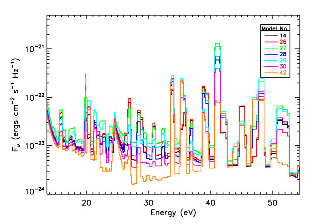
Figure 2: Model ionizing radiation fields for several different models from Slavin and Frisch (2008), all of which match the observational constraints.

We find successful models for range of values for $N(\mathrm{H\,I})$ towards $\epsilon$CMa and $T$(hot gas). Our results for the Solar location are:

• $n(\mathrm{H}^{0})=0.19-0.20$ cm^-3,

• $n_{e}=0.07\pm 0.01$ cm^-3,

• $n(\mathrm{H})=0.23-0.27$ cm^-3,

• $B=2.1,2.5\mu$G for two best models (the magnetic field affects emission intensity from cloud boundary).

3 Dust and Elemental Abundances in the LIC

Our approach to modeling the abundances in the LIC is to force our models to match the column densities observed by adjusting the elemental abundances. Thus the abundances are an output of the modeling rather than in input. Figure 3 illustrates the abundance results for C, N, O, S, Si, Mg and Fe relative to a particular assumed solar abundance of the elements (Asplund et al., 2005). The x-axis is the condensation temperature for the element, a quantity often presumed to correlate with the amount of depletion from the gas phase. In Table 1 we list the derived abundances in our models that are consistent with observations.

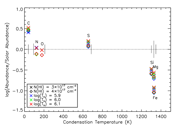
Figure 3: Abundances relative to Asplund et al. (2005) solar abundances vs. condensation temperature. Results from models of the ionization for the $\epsilon$ CMa line of sight including radiative transfer (Slavin and Frisch, 2008). The symbol shape indicates the assumed H i column density for the model, while the color indicates the assumed temperature for the hot gas of the Local Bubble. The abundances are fixed so as to match the observed ion column densities.

Table 1: Elemental Gas Phase Abundances (ppm)

	Element
Model No.	C	N	O	Mg	Si	S	Fe
14	589	40.7	295	5.89	7.24	14.1	2.24
25	631	66.1	437	7.76	10.0	19.5	3.09
26	661	46.8	331	6.61	8.13	15.8	2.51
27	759	64.6	437	8.71	10.7	20.9	3.31
28	708	45.7	331	7.08	8.32	16.6	2.57
29	813	64.6	437	9.33	11.0	21.9	3.39
30	741	46.8	331	7.41	8.51	17.0	2.63
42	724	39.8	295	6.76	7.76	15.1	2.34

The derived abundances indicate modest depletion of the constituents of silicate dust, Si, Fe, Mg, and O, implying that at least some destruction of this type of dust. Depending on ones assumptions about the initial depletion of Si (Savage and Sembach, 1996, quote values of 70-95%), the total Solar abundance of Si (recent determinations range from about 30 to 43 ppm) and its current gas phase abundance (we find $\sim 7.2-11.5$ ppm) the fraction of the silicate grain mass destroyed (i.e. returned to the gas phase) ranges from 0 to 35%. The high C abundance on the other hand seems to indicate that all the carbonaceous dust has been destroyed. Radiative shocks destroy dust via various processes: sputtering, vaporization, shattering. Detailed calculations by Jones et al. (1996) find that silicate dust should be more destroyed than carbonaceous dust by shocks, as illustrated in Figure 4. Therefore either some other process is strongly influencing the gas phase abundances in the LIC or the models of shock processing of grains need revision.

Figure 4: Percentage of initial total grain mass lost because of dust destruction in the shock vs. shock speed. To get the Si gas phase abundance determined for the LIC we need $\lesssim$35% destruction of silicate dust which is consistent with $v_{\mathrm{shock}}\lesssim 150$ km s^-1. Such shocks should destroy less than 15% of the cabonaceous dust, however, in contradiction with the derived large gas phase abundance of C.

4 LIC Ionization and Thermal Balance

Observations with the Extreme Ultraviolet Explorer (EUVE) toward nearby stars found unexpected results for the ratio of H i to He i column density (Dupuis et al., 1995). Instead of the expected ratio of $\leq 10$ that one would get if the cosmic He abundance is 0.1 and H is more ionized than He, it was found that $N(\mathrm{H\,I})/N(\mathrm{He\,I})\sim 14$, indicating that He is more ionized than H. This unusual ionization of the local ISM has long been considered puzzling and has led to the suggestion that the LIC is out of ionization equilibrium, being overionized for its temperature because of an earlier ionizing event (e.g. a shock) (see, e.g., Lyu and Bruhweiler, 1996). The long timescale for recombination, particularly of H, it was reasoned, makes it likely that the LIC is out of ionization equilibrium. However, the cooling rate of the gas also has to be considered in such a model. Doing this one finds that in fact the cooling time for the gas in any likely scenario is considerably less than the recombination time. As a result, if the LIC were cooling from a hotter and more ionized state, it should still be quite highly ionized by the time that it has cooled to the observed temperature of $T\approx 6300$ K. In Figure 5 we illustrate this by showing the temperature and ionization evolution behind a 100 km s^-1 shock. Even greater disparity between the cooling time and recombination time is found for a simple isobaric cooling model. Therefore the fact that the LIC is in fact mostly neutral, $X(\mathrm{H}^{+})\sim 0.2$, implies that the cloud has had time to recombine while being maintained at a warm temperature. This requires a heat source to balance the cooling. While alternative sources have been proposed, such as turbulent dissipation (Minter and Spangler, 1997), the most likely heat source appears to be photoionization heating. Such heating is also accompanied by ionization, suggesting that the cloud is at least close to thermal and photoionization equilibrium.

Figure 5: Time evolution of temperature and H ion fraction behind a 100 km s^-1 shock (J. Raymond, private communication). The dotted lines show the time, temperature and H ion fraction when the gas cools to the LIC temperature, while the dashed lines show the same for the LIC H ion fraction. Isobaric cooling shows a similar lag of H recombination. The gas cools too fast to allow the relatively low degree of ionization in the LIC at temperatures of $\sim 6300$ K without some substantial heating source.

Another argument in favor of the cloud being in ionization equilibrium was first suggested by Jenkins et al. (2000) based on Ar i and O i data. Since O ionization is tied to H ionization by charge exchange, if we assume an O abundance we can then compare the ionization of Ar and H. In recombining gas, it is found that Ar and H have roughly equal ionization fractions because H⁺ and Ar⁺ have similar recombination coefficients. However, for gas in photoionization equilibrium, Ar i is deficient relative to H i (or Oi) because the photoionization cross section for Ar⁰ is 5-30 times larger than that for H⁰. Observations for the LIC (Jenkins et al., 2000) find $X(\mathrm{Ar}^{0})/X(\mathrm{H}^{0})\sim 0.4$ toward nearby white dwarfs. Detailed NEI calculations for cooling gas show that $X(\mathrm{Ar}^{0})/X(\mathrm{H}^{0})$ remains $\sim 1$ until gas nears equilibrium and is photoionized.

Despite this evidence that the LIC is currently close to ionization and thermal equilibrium, there are reasons to believe that it has not always been so. The LIC is clearly many times denser than its surrounding gas in the Local Bubble as can be deduced from the low absorption by neutral gas within the bubble and lack of observable optical emission from possible warm ionized gas that could conceivably fill the cavity. That leaves only highly ionized and very low density gas as the primary volume filling gas in the bubble. Therefore it appears highly likely that the gas that presently makes up the LIC and other nearby clouds was at one time substantially overdense compared with the surrounding medium before becoming incorporated into the Local Bubble. The most likely scenario is that cold neutral medium gas, with $n\sim 100$ cm^-3, $T\sim 100$ K, that was embedded in warm gas was hit by a shock. However, it is important to note that any shock no matter what speed hitting such a dense cloud will go radiative in the cloud. Thus one needs to find a means to heat the cloud to warm neutral medium temperatures. An origin in a fragmented shell implies a similar radiative shock and heating requirements. The means to heat the shocked warm clouds seems to require their expansion to lower density as the pressure of the bubble drops at the same time as ionizing flux from the hot gas and possibly from the cloud boundary regions provides heating.

For diffuse ISM conditions, calculated heating and cooling rates typically lead to the possibility of thermal balance with two stable thermal phases within a limited range of thermal pressures, with a cold neutral phase and a warm neutral or (perhaps partially) ionized phase. Figure 6 shows a density vs. pressure plot or phase diagram showing two different phase equilibrium curves. The one for “Low Ionization” comes from the work of Wolfire et al. (2003) and assumes low ionizing flux whereas the “LIC ionization” one is calculated using one of our model ionizing radiation fields for the LIC. We note that the thermal pressure will generally not dominate the total dynamical pressure because other pressure forms including magnetic, cosmic ray and turbulent, are typically estimated to be of the same order of magnitude as the thermal pressure. This does not affect the phase curves, however, since it is the components of the thermal pressure (i.e. density and temperature) that directly affect the heating-cooling balance. In the diffuse ISM cosmic ray heating is small compared to dust and photoionization heating. It may be that turbulent dissipation, particularly in concert with MHD turbulence, provides significant heating, however the rate for that remains quite uncertain and is neglected in the Figure.

The arrows on the plot indicate how gas parcels will evolve under the influence of shocks, adiabatic cooling (cooling via expansion) and evaporation via thermal conduction. The shock arrow indicates a relatively small increase in pressure, which would require only a mach 2.5 (relative to the cold gas) shock. A shock that could heat typical warm (ionized or neutral) medium gas to about $10^{6}$ K would need to be much faster, $v_{s}\approx 270$ km s^-1, or mach 27 in the warm medium. The pressure would thus be increased to $P/k_{B}\sim 2\times 10^{6}$ cm^-3 K. In order for the local clouds to become warm would require the pressure to drop by more than two orders of magnitude after the shock passed over them. This could be achieved after sufficient expansion, e.g. a factor of $\sim 4$ in radius assuming adiabatic expansion of a spherical bubble. This requires that the clouds were close enough to the center of the superbubble that the shock had not gone radiative yet and that the clouds (or at least a fraction of them) could survive long enough to persist until our current state in which the surrounding bubble has a relatively low pressure.

Figure 6: Phase diagram for the diffuse interstellar medium for either low ionizing flux conditions (dashed curve, using rates from Wolfire et al., 2003) or the moderate ionizing flux as modeled for the LIC (solid curve using our modeled radiation field). Points on the curve are conditions of thermal equilibrium, below the curve heating exceeds cooling and above the curve cooling exceeds heating. The diagonal lines are curves of constant temperature. A shock will tend to move a gas parcel up and to the right in the diagram, while adiabatic cooling moves points down and to the left as illustrated by the arrows. Evaporation via thermal conduction moves points to left. Note that the pressure in the plot is only thermal pressure and thus neglects the dynamically important magnetic, cosmic ray and turbulent pressures in the ISM.

5 The Origin the Complex of Local Interstellar Clouds

The above discussion lays out some of the challenges facing any model for the origin of the complex of local interstellar clouds. In summary we would like a theory to explain these facts:

• The density, temperature and ionization of the clouds are in sharp contrast to the surrounding Local Bubble gas (though we don’t know all the properties of that gas),

• the CLIC has a significant velocity relative to the LSR and direction roughly away from Galactic center,

• the ionization of the LIC is unusual with He apparently more ionized than H,

• the abundances in the gas seem to imply that carbonaceous dust has been destroyed, and yet interstellar dust observed in the Solar System implies a relatively low gas-to-dust ratio.

A number of theories have been put forward to explain the CLIC. The clouds have been variously proposed to be: 1) pieces of the Sco-Cen bubble from an earlier epoch of star formation (Frisch, 1981), 2) a fragment from Sco-Cen/LB interaction (Breitschwerdt et al., 2000), and 3) a flux tube/filament that has broken away from the bubble wall (Cox and Helenius, 2003). We would add to this list, 4) a dense cloud in the ambient medium overrun by an expanding bubble shock, a model that we have discussed briefly above but that has yet to be fully explored.

Each of these models has its problems. The velocity and relative positions of the CLIC and Loop I bubble strongly suggest a connection between them but detailed modeling of how these clouds could have come from that bubble is lacking. Breitschwerdt et al. (2000) propose that the Local Bubble and the Loop I bubble are interacting and that the CLIC is associated with the wall that separates the bubbles. In their model the clouds are created by instabilities generated in the interaction region. The LIC is currently about 70 pc from that neutral wall and moving about 20 km s^-1 away from the Sco-Cen association that is believed to be responsible for creating the Loop I bubble. It is unclear how cloudlets like the CLIC could have been traveling for 3.5 million years away from this interaction zone and yet the wall is apparently intact between the two bubbles. Frisch (1981) suggests that the clouds as well as the Local Bubble are associated with a previous epoch of star formation of Sco-Cen. This requires that somehow a cold neutral wall was reformed within the bubble between these epochs of star formation. The mechanism for doing that is left unexplained. The flux tube theory of the origins of the CLIC by Cox and Helenius (2003) requires that a flux tube sprang from the wall of the Local Bubble pulling warm gas along with it into the bubble interior. The magnetohydrodynamics of this explanation seem questionable however, in particular that one flux tube can spring from the bubble wall while the rest of the bubble is not collapsing. Finally, our idea that the clouds originated as cold clouds in a warm intercloud medium seems reasonable but does not explain why the velocity of the CLIC is directed away from the Sco-Cen association and towards the center of the Local Bubble rather than away from it. We must appeal to a random velocity of the gas prior to being overrun by the expanding Local Bubble to explain this.

6 Summary

The wide range of data that we have on the LIC has lead to a fairly complete picture of the cloud. We find that it is:

• partially ionized, $X(\mathrm{H}^{+})\sim 0.2-0.3$, $X(\mathrm{He}^{+})\sim 0.3-0.4$, $n_{e}\approx 0.07$ cm^-3

• has experienced mixed dust destruction – moderate for silicate dust, complete for carbonaceous,

• at or close to ionization equilibrium

An origin as a cloud embedded in a lower density medium that was shocked seems likely, and some association with the Loop I bubble and Sco-Cen OB association remains a possibility. Many mysteries remain about its abundances and origins within the local ISM.