Constraints on the non-linear coupling parameter $f_{nl}$ with Archeops data

Abstract

Aims. We present a Gaussianity analysis of the Archeops Cosmic Microwave Background (CMB) temperature anisotropy data maps at high resolution to constrain the non-linear coupling parameter $f_{nl}$ characterising well motivated non-Gaussian CMB models. We used the data collected by the most sensitive Archeops bolometer at 143 GHz. The instrumental noise was carefully characterised for this bolometer, and for another Archeops bolometer at 143 GHz used for comparison. Angular scales from 27 arcmin to 1.8 degrees and a large fraction of the sky, 21%, covering both hemispheres (avoiding pixels with Galactic latitude $|b|<15$ degrees) were considered.

Methods. The three Minkowski functionals on the sphere evaluated at different thresholds were used to construct a $\chi^{2}$ statistics for both the Gaussian and the non-Gaussian CMB models. The Archeops maps were produced with the Mirage optimal map-making procedure from processed time ordered data. The analysis is based on simulations of signal (Gaussian and non-Gaussian $f_{nl}$ CMB models) and noise which were processed in the time domain using the Archeops pipeline and projected on the sky using the Mirage optimal map-making procedure.

Results. The Archeops data were found to be compatible with Gaussianity after removal of highly noisy pixels at high resolution. The non-linear coupling parameter was constrained to $f_{nl}=70_{-400}^{+590}$ at 68% CL and $f_{nl}=70_{-920}^{+1075}$ at 95% CL, for realistic non-Gaussian CMB simulations.

1 Introduction

The Cosmic Microwave Background (CMB) radiation is a valuable tool to study the early universe. When we observe this weak radiation we are observing the universe when it was about 400000 years old. Several theories have been proposed to explain the origin and the evolution of the universe. The Big Bang is the most favored theory and it predicts the existence of the CMB. The inflationary models are complementary to the Big Bang model. Among their many properties we are interested in those related to the CMB and the predictions that they present about it. The standard, single field, slow roll inflation (Guth 1981; Albrecht & Steinhardt 1982; Linde 1982, 1983) is one of the most accepted models because of the accuracy of its predictions and the observations performed with modern experiments (Spergel et al. 2007). In particular, the standard inflation predicts that the primordial density fluctuations are distributed following a nearly Gaussian distribution. These fluctuations are imprinted in the anisotropies of the CMB. Therefore if the prediction is correct the anisotropies of the CMB should be distributed in a nearly Gaussian way. Any detection of non-Gaussian deviations would have far-reaching consequences for our understanding of the Universe (Cruz et al. 2007b; Yadav & Wandelt 2007). In addition the search for non-Gaussian fluctuations in the data is a useful tool to look for residual foreground, secondary anisotropies or unidentified systematic errors. Some of these effects may introduce non-Gaussian features at different levels.

Many statistical tools have been applied to test the Gaussianity of CMB data sets. The Minkowski functionals have been applied to different recent experiments (Spergel et al. 2007; de Troia et al. 2007; Gott et al. 2007; Curto et al. 2007); other examples are the smooth tests of goodness-of-fit (Cayón et al. 2003b; Aliaga et al. 2005; Rubiño-Martín et al. 2006; Curto et al. 2007), wavelets (Barreiro et al. 2000; Cayón et al. 2001; Vielva et al. 2004; Mukherjee & Wang 2004; Cruz et al. 2005, 2007a), local estimators of the n-point correlations (Eriksen et al. 2004, 2005), steerable filters (Wiaux et al. 2006; Vielva et al. 2007), and the CMB 1-pdf (Monteserín et al. 2007) among others.

In this work we analyse the CMB data collected by the Archeops experiment. Important results have been obtained from this experiment since its launch in 2002. It gave the first link in the $C_{\ell}$ determination (Benoît et al. 2003a) between the COBE large angular scale data (Smoot et al. 1992) and the first acoustic peak as measured by BOOMERanG and MAXIMA (de Bernardis et al. 2000; Hanany et al. 2000). From this it gave a precise determination of the main cosmological parameters (Benoît et al. 2003b). It also provided an independent confirmation at different frequencies of the power spectrum for the range $\ell=10$ to $\ell=700$ of the WMAP first year results (Tristram et al. 2005).

In this study we use the Minkowski functionals (Minkowski 1903; Gott et al. 1990; Schmalzing & Górski 1998). This new Gaussianity analysis of the Archeops data complements the first analysis presented in Curto et al. (2007) where only low resolution maps (about 1.8 degrees of resolution) were analysed and the $f_{nl}$ constraints were imposed on non-Gaussian CMB maps simulated using the quadratic Sachs-Wolfe approximation. In contrast, in the present work, the constraints on the non-linear coupling parameter $f_{nl}$ are obtained using higher resolution (27 arcmin) Archeops data and realistic non-Gaussian simulations of the CMB fluctuations with the algorithms developed by Liguori et al. (2003, 2007).

Our article is organized as follows. Section 2 presents the Archeops data and the Gaussian and non-Gaussian simulations performed. Section 3 describes the statistical methods to test Gaussianity and to constrain the $f_{nl}$ parameter. In Section 4 we perform an analysis of the instrumental noise which will provide the correct masks for our analysis. Section 5 is devoted to the $f_{nl}$ constraints and the comparison with the Sachs-Wolfe approximation. We summarize and draw our conclusions in Section 6.

2 Data and simulations

2.1 The data

Archeops is a balloon-borne experiment to map the CMB anisotropies at high resolution with a large sky coverage. The experiment is described in Benoît et al. (2002, 2004a, 2004b); Macías-Pérez et al. (2007). It is based on the Planck high frequency instrument (HFI) technology. The instrument consists of a 1.5 m telescope pointing at 49 degrees from its vertical axis on board a stratospheric gondola. It has 21 bolometers cooled to 100 mK by an ³He/⁴He dilution cryostat designed to work at similar conditions to the ones expected for Planck. These bolometers operate at frequencies of 143, 217, 353 and 545 GHz. After one test flight in Trapani (Italy), the instrument flew three times from the CNES/Swedish facility of Esrange, near Kiruna (Sweden) to Siberia (Russia). The last flight on February $7^{th}$ 2002 provided 12.5h of CMB-quality data for a total of 19h. The experiment was performed during the Arctic winter to avoid Sun contamination. These data correspond to a sky coverage of approximately 30% of the sky, including the Galactic plane. From its four frequency bands the two lowest (143 and 217 GHz) were dedicated to the observation of the CMB and the others (353 and 545 GHz) to the monitoring and calibration of both atmospheric and Galactic emission.

We used the data collected with two bolometers at 143 GHz. We used the data of the $143K03$ bolometer for the main analysis (see Sect. 5) and the data of the $143K03$ and $143K04$ bolometers for the noise analysis (see Sect. 4). However, for the $f_{nl}$ constraints, the data from the second bolometer $143K04$ are not used due to their higher noise level and worse systematic errors. The characteristics of the bolometers are described in Macías-Pérez et al. (2007). In Curto et al. (2007) the Gaussianity analysis of Archeops data was performed at low resolution, in particular HEALPix (Górski et al. 2005) $N_{side}=$ 32. Here we complement that work and analyse the data at the same and higher resolutions: $N_{side}=$ 32, 64, and 128 using the realistic non-Gaussian simulations presented below.

First we processed and cleaned the Time Ordered Information (hereafter TOI) as described in Tristram et al. (2005). Then the data maps at different resolutions were produced using the Mirage optimal map-making procedure (Yvon & Mayet 2005). All the analyses presented here were performed on a fraction of the Archeops observed region after masking out pixels with Galactic latitude $|b|<15^{o}$. This corresponds to 21% of the total sky. Unlike the analysis in Curto et al. (2007), restricted to north Galactic latitudes, south Galactic latitudes are included in the analysis.

2.2 Gaussian simulations

We have performed Gaussian simulations of the CMB signal and of the Archeops noise as described in Curto et al. (2007). The noise simulations were obtained from Gaussian random realisations of the time-domain noise power spectrum of the bolometers. The constructed noise time ordered data were then projected using the Mirage optimal map-making procedure. The CMB Gaussian simulations were obtained from random realisations of the best–fit Archeops CMB power spectrum. From these maps we constructed Archeops time ordered data and then we project them using Mirage. In this way, the filtering of the Archeops data was taken into account.

2.3 Non-Gaussian CMB simulations

There are several alternative theories to the standard inflation theory that introduce non-Gaussian fluctuations in the CMB. One simple model that describes weakly non-Gaussian fluctuations in matter and radiation is obtained by introducing a quadratic term in the primordial gravitational potential (Salopek & Bond 1990; Gangui et al. 1994; Verde et al. 2000; Komatsu & Spergel 2001)

$$\Phi(\@vec{x})=\Phi_{L}(\@vec{x})+f_{nl}\{\Phi_{L}^{2}(\@vec{x})-\langle\Phi_{L}^{2}(\@vec{x})\rangle\}\ \$$ (1)

where $\Phi_{L}(\@vec{x})$ is a linear random field which is Gaussian distributed and has zero mean, and $f_{nl}$ is is the non-linear coupling parameter. Non-Gaussianity of this type is generated in various classes of non-standard inflationary models (see, e. g. Bartolo et al. 2004, for a review). To obtain the CMB anisotropies generated by such a primordial gravitational potential we use the algorithm described in Liguori et al. (2003) for the temperature maps or Liguori et al. (2007) for temperature and polarization maps.

In this case the multipole coefficients $a_{lm}$ of the CMB temperature map can be written as

$$a_{lm}=a_{lm}^{(G)}+f_{nl}a_{lm}^{(NG)}$$ (2)

where $a_{lm}^{(G)}$ is the Gaussian contribution and $a_{lm}^{(NG)}$ is the non-Gaussian contribution.

For our simulations we use the $\Lambda$CDM model that best fits the WMAP data and a modified version of the CMBFAST code (Seljak & Zaldarriaga 1996) to obtain the Gaussian and non-Gaussian contributions as described above. We produced a set of 300 high resolution full sky temperature Gaussian maps $\Delta T_{G}$ and their complementary non-Gaussian maps $\Delta T_{NG}$ at the same resolution. The total CMB map with a non-Gaussian contribution is therefore

$$\Delta T=\Delta T_{G}+f_{nl}\Delta T_{NG}.$$ (3)

To constrain $f_{nl}$ with Archeops data we need to transform these simulations into Archeops simulations. For this purpose, each simulated non-Gaussian map given by Eq. 3 was converted into Archeops time-ordered data accounting for the Archeops pointing. These time-ordered data were re-normalised to account for intercalibration errors between Archeops and WMAP, and added to Gaussian simulations of the Archeops instrumental noise constructed as above. Then the time ordered data was projected on the sky using Mirage. Although, the Mirage algorithm is weakly non-linear, i.e., the map obtained from $\Delta T_{G}$ and $\Delta T_{NG}$ separately is slightly different from the one obtained from the sum of the two contributions, we have tested that the Minkowski functionals are very similar in both cases. Thus, for our analysis, we can construct the Archeops simulations for different values of $f_{nl}$ by adding the Mirage map for $\Delta T_{G}$ to the one for $\Delta T_{NG}$ multiplied by $f_{nl}$. This corresponds to an important saving of CPU time as the Mirage algorithm is a significantly time consuming process (Curto et al. 2007).

Thus, we transformed our sets of 300 $\Delta T_{G}$ and $\Delta T_{NG}$ simulations into CMB Archeops simulations ($s_{g}$ and $s_{ng}$) at the three considered resolutions $N_{side}=$32, 64, and 128. The final non-Gaussian simulations accounting for $f_{nl}$ were computed from $s_{g}+f_{nl}s_{ng}+n_{g}$ where $n_{g}$ corresponds to the Archeops Gaussian noise simulations.

3 Methodology

The Gaussianity analysis and the constraints on the $f_{nl}$ parameter were performed using the Minkowski functionals. Detailed theoretical information about these quantities is presented for example in Gott et al. (1990); Schmalzing & Górski (1998). Some recent examples of applications of the Minkowski functionals to the CMB are in Curto et al. (2007) for Archeops data at low angular resolution, de Troia et al. (2007) for BOOMERanG 2003 data, and Spergel et al. (2007) for WMAP 3rd year data.

For a scalar field $\Delta T(\@vec{n})$ in the sphere we have three Minkowski functionals given a threshold $\nu$. Considering the excursion set of points $Q_{\nu}$ where $\Delta T(\@vec{n})/\sigma>\nu$ the three Minkowski functionals are: the area $A(\nu)$ of $Q_{\nu}$, the contour length $C(\nu)$ of $Q_{\nu}$, and the genus $G(\nu)$ (proportional to the difference between hot spots above $\nu$ and cold spots below $\nu$). The expected values of the functionals for a Gaussian random field are (Schmalzing & Górski 1998)

$$\langle A(\nu)\rangle = \frac{1}{2}\left(1-\frac{2}{\sqrt{\pi}}\int_{0}^{\nu/\sqrt{2}}exp(-t^{2})dt\right)$$

$$\langle C(\nu)\rangle = \frac{\sqrt{\tau}}{8}exp\left(-\frac{\nu^{2}}{2}\right)$$

$$\langle G(\nu)\rangle = \frac{\tau}{(2\pi)^{3/2}}\leavevmode\nobreak\ \nu\leavevmode\nobreak\ exp\left(-\frac{\nu^{2}}{2}\right)$$

where $\sigma=\sum_{\ell=1}^{\ell_{max}}(2\ell+1)C_{\ell}$ and $\tau=\sum_{\ell=1}^{\ell_{max}}(2\ell+1)C_{\ell}\ell(\ell+1)/2$. These expressions are only valid in an ideal case. In practice, we will obtain these quantities from Gaussian CMB simulations in order to take into account the noise, mask and pixel effects.

For a Gaussian random field the Minkowski functionals are approximately Gaussian distributed, therefore we can use a $\chi^{2}$ statistic to test the Gaussianity of a CMB map. This statistic is computed with the three Minkowski functionals evaluated at $n_{th}$ different thresholds.

$$\chi^{2}=\sum_{i,j=1}^{3n_{th}}(v_{i}-\langle v_{i}\rangle)C_{ij}^{-1}(v_{j}-\langle v_{j}\rangle)$$ (5)

where $\langle\rangle$ is the expected value for the Gaussian case, $\@vec{v}$ is a $3n_{th}$ vector

$$(A(\nu_{1}),..,A(\nu_{n_{th}}),C(\nu_{1}),..,C(\nu_{n_{th}}),G(\nu_{1}),..,G(\nu_{n_{th}})),$$ (6)

and $C$ is a $3n_{th}$ covariance matrix

$$C_{ij}=\langle v_{i}v_{j}\rangle-\langle v_{i}\rangle\langle v_{j}\rangle.$$ (7)

The Gaussianity analysis consists of computing the $\chi^{2}$ statistic of the data and compare it with the value of the $\chi^{2}$ statistic of a set of Gaussian simulations of the data (CMB signal plus instrumental noise).

Another important analysis is the estimation of the $f_{nl}$ parameter. In this case, we can use a $\chi^{2}$ test with the Minkowski functionals

$$\chi^{2}(f_{nl})=\sum_{i,j=1}^{3n_{th}}(v_{i}-\langle v_{i}\rangle_{f_{nl}})C_{ij}^{-1}(f_{nl})(v_{j}-\langle v_{j}\rangle_{f_{nl}})$$ (8)

where $\langle\rangle_{f_{nl}}$ is the expected value for a model with $f_{nl}$, and $C_{ij}(f_{nl})=\langle v_{i}v_{j}\rangle_{f_{nl}}-\langle v_{i}\rangle_{f_{nl}}\langle v_{j}\rangle_{f_{nl}}$. For low values of $f_{nl}$ ($f_{nl}\mathrel{\mathchoice{\lower 3.6pt\vbox{\halign{$\mathsurround=0pt\displaystyle\hfil#\hfil$\cr<\crcr\sim\crcr}}}{\lower 3.6pt\vbox{\halign{$\mathsurround=0pt\textstyle\hfil#\hfil$\cr<\crcr\sim\crcr}}}{\lower 3.6pt\vbox{\halign{$\mathsurround=0pt\scriptstyle\hfil#\hfil$\cr<\crcr\sim\crcr}}}{\lower 3.6pt\vbox{\halign{$\mathsurround=0pt\scriptscriptstyle\hfil#\hfil$\cr<\crcr\sim\crcr}}}}1500$) we have that $C_{ij}(f_{nl})\simeq C_{ij}(f_{nl}=0)=C_{ij}$, and therefore we can use the approximation

$$\chi^{2}(f_{nl})=\sum_{i,j=1}^{3n_{th}}(v_{i}-\langle v_{i}\rangle_{f_{nl}})C_{ij}^{-1}(v_{j}-\langle v_{j}\rangle_{f_{nl}}).$$ (9)

The best-fit $f_{nl}$ for the Archeops data is obtained by minimization of $\chi^{2}(f_{nl})$. Error bars for it at diffirent confidence levels are computed using the Gaussian simulations.

Other than the analysis of the data at each resolution separately we can also analyse the data by combining the information at different resolutions. Assuming maps at $n_{res}$ different resolutions we can define a vector

$$\@vec{V}=(\@vec{v}_{1},\@vec{v}_{2},...,\@vec{v}_{n_{res}}),$$ (10)

where each $v_{i}$ corresponds to the vector given by Eq. 6 for the resolution $i$. With this combined vector we can compute $\chi^{2}$ statistics in the same way as in Eqs. 5 and 9

$$\chi^{2} = \sum_{i,j=1}^{3N_{th}}(V_{i}-\langle V_{i}\rangle)C_{ij}^{-1}(V_{j}-\langle V_{j}\rangle)$$ (11)

$$\chi^{2}(f_{nl}) = \sum_{i,j=1}^{3N_{th}}(V_{i}-\langle V_{i}\rangle_{f_{nl}})C_{ij}^{-1}(V_{j}-\langle V_{j}\rangle_{f_{nl}})$$ (12)

where $\langle\rangle$ is the expected value for the Gaussian case, $\langle\rangle_{f_{nl}}$ is the expected value for a model with $f_{nl}$, $N_{th}=\sum_{k=1}^{n_{res}}n_{th}^{(k)}$, $n_{th}^{(k)}$ is the number of thresholds used at resolution $k$, and $C_{ij}=\langle V_{i}V_{j}\rangle-\langle V_{i}\rangle\langle V_{j}\rangle$.

4 Gaussianity analysis of the Archeops instrumental noise

Figure 1: Distribution of the $\chi^{2}$ values from the Minkowski Gaussianity analysis for the Archeops 143K03-143K04 map at $N_{side}=32$, $N_{side}=64$, and $N_{side}=128$. The vertical lines show data, the histograms are obtained from a set of $10^{3}$ simulations, and the solid lines are the expected $\chi^{2}$ distributions for $3n_{th}$ degrees of freedom.

Figure 2: Distribution of the $\chi^{2}$ values from the Minkowski Gaussianity analysis for the Archeops 143K03 noise map at $N_{side}=32$, $N_{side}=64$, and $N_{side}=128$. Vertical lines show data, the histograms corresponds to sets of $10^{3}$ noise simulations, and the solid lines are the $\chi^{2}$ distribution with $3n_{th}$ degrees of freedom.

Figure 3: From left to right, $\chi^{2}$ statistic of the 143K03 noise map, its cumulative probability, and the fraction of available area for different values of the minimum number of hits at $N_{side}=128$. This map becomes compatible with Gaussianity when the minimum number of hits is approximately 90.

From Macías-Pérez et al. (2007) it is expected that the noise at a given pixel behaves as Gaussian when the pixel has been observed a sufficiently large number of times, about 100 times. In order to check the noise behaviour, we perform a Gaussianity analysis of the Archeops instrumental noise. This is needed to exclude from the main Gaussianity analysis the possible scales and regions of the sky where the Archeops noise is non-Gaussian.

4.1 Two bolometer analysis

A simple way to analyse the instrumental noise is to subtract the data of two different bolometers at the same frequency so that the sky signal is removed in the final map. We used the data collected by two different Archeops bolometers at 143 GHz: 143K03 and 143K04. As the CMB contribution is the same for both bolometers but the noise is not, after subtraction and assuming no systematic errors only the noise contributions remain. Defining $d_{K03}$ as the data collected by 143K03 and $d_{K04}$ the data collected by 143K04, the map that we analysed is

$$d=d_{K03}-d_{K04}\approx n_{K03}-n_{K04}.$$ (13)

We analysed the difference data maps given by Eq. 13 for three different resolutions: $N_{side}=32$, $N_{side}=64$, and $N_{side}=128$. To construct simulations of the difference map, we used a set of $10^{3}$ Gaussian signal simulations and $10^{3}$ Gaussian noise simulations for each bolometer and each resolution. These simulations are used to compute the mean value $\langle v_{i}\rangle$ and the covariance matrix $C_{ij}$ of the Minkowki functionals as described in Sect. 3.

In Fig. 1 we present, from left to right, the Gaussianity analysis of the difference maps at the three resolution considered, $N_{side}=32$, $N_{side}=64$, and $N_{side}=128$. The histograms correspond to the values of the $\chi^{2}$ obtained for $10^{3}$ simulations of difference maps. The vertical lines correspond to the value of $\chi^{2}$ for the Archeops data. The solid lines are the theoretical $\chi_{3n_{th}}^{2}$ distribution normalised to the number of simulations and the size of the binned cell.

From this analysis we can see that the data given by Eq. 13 becomes non-Gaussian at high resolution. This is most probably due to highly noisy pixels in the difference maps corresponding to regions of the sky observed with little redundancy. A previous analysis (Macías-Pérez et al. 2007) has shown that the Archeops instrumental noise in the map domain is Gaussian distributed for a given pixel when this pixel has been observed a significant amount of time, typically above a few hundred independent observations (hits) per pixel, although no precise estimate of the required number of hits per pixel was given.

This can be easily done using the statistical tools presented in this paper. For this purpose we perform our analysis excluding highly noisy pixels defined as those pixels presenting a number of hits below a given threshold. We computed the $\chi^{2}$ statistic of the data (Eq. 13), its cumulative probability, and the remaining area using different thresholds for the number of hits. By comparing to the Gaussian simulations we observe that for both $N_{side}=64$ and $N_{side}=128$, increasing the threshold of the number of hits implies that the data becomes compatible with Gaussianity. In particular, for $N_{side}=64$ the data become compatible with Gaussianity when pixels with fewer than 250 hits are removed (leaving $46\%$ of the original area) and for $N_{side}=128$ the data start to become compatible with Gaussianity when pixels with fewer than 150 hits are removed (leaving $13\%$ of the original area).

4.2 Single bolometer analysis

From the above analysis we have proved that highly noisy pixels are responsible for the non-Gaussianity of the Archeops noise at high resolution. In order to obtain proper limits for the $f_{nl}$ parameter we need to exclude these pixels in our final analysis of the $143K03$ map.

To avoid any contamination from the $143K04$ noise map when characterizing the noise map for the 143K03 bolometer the latter was computed using the WMAP data as follows

$$n_{K03}=d_{K03}-WMAP_{K03}*f$$ (14)

where $WMAP_{K03}$ is the combined WMAP data computed as described in Curto et al. (2007) and converted into an Archeops map as described in Sect. 2.3. $f$ is an intercalibration parameter between WMAP and Archeops, $f=1/1.07$, as given by Tristram et al. (2005). In this case, as the noise on the WMAP data at the considered map resolutions is negligible compared to the Archeops noise, we expect no contamination.

We analysed the noise map given by Eq. 14 for three different pixel resolutions: $N_{side}=32$, $N_{side}=64$, and $N_{side}=128$. For each resolution, we also analysed a set of $10^{3}$ Archeops noise simulations $n_{K03}$. The results are presented in Fig. 2. The histograms correspond to the $\chi^{2}$ of the Minkowski functionals of a set of $10^{3}$ $n_{K03}$ Gaussian simulations, vertical lines correspond to the data maps given by Eq. 14 and the solid lines are the $\chi^{2}_{3n_{th}}$ distributions. We can see that for low resolution ($N_{side}=32$ and $N_{side}=64$) the noise map is compatible with the Gaussian noise simulations. Therefore for these two resolutions we can use the full available area in the $f_{nl}$ analysis.

In the case of $N_{side}=128$ the noise map is not compatible with Gaussianity. As above, we reanalysed this noise map removing highly noisy pixels with a number of hits below a given threshold. This analsysis is presented in Fig. 3 where from left to right we plot the $\chi^{2}$ statistic of the 143K03 noise map, its cumulative probability, and the fraction of available area for different values of the minimum number of hits. We can see that the Archeops noise for the $143K03$ bolometer becomes clearly Gaussian when we remove pixels with a number of hits lower than 90. This means that the area where the noise is Gaussian is $32\%$ of the original area at $N_{side}=128$. In conclusion, the regions of the sky that we can use for the Gaussianity analysis are the whole initial area at $N_{side}=32$ and $N_{side}=64$ and $32\%$ of the initial area at $N_{side}=128$.

The $143K04$ bolometer has a qualitatively similar behaviour for the noise analysis. That is, the noise map is compatible with Gaussianity at low resolution and is non-Gaussian at high resolution. Nevertheless as the noise for this bolometer has more systematic errors than the $143K03$ bolometer, the thresholds for the number of hits where the maps become compatible with Gaussianity analysis are higher. This implies that the available area where the noise is Gaussian is smaller.

5 Results

In this section, we perform the Gaussianity analysis of the $143K03$ Archeops bolometer data in order to constrain the non-linear coupling parameter, $f_{nl}$. For this, we first consider realistic non-Gaussian simulations as described in Sect. 2.3. Then the results are compared to the ones obtained for non-Gaussian simulations for which only the Sachs-Wolfe contribution is included, as in Curto et al. (2007).

5.1 Gaussianity analysis

Figure 4: From left to right, and from top to bottom, the area, contour length, and genus of the data (asterisk *) as a function of threshold for the 143K03 maps with $N_{side}=32$, $N_{side}=64$, and $N_{side}=128$. We also plot the acceptance intervals for the 68% (inner in red), the 95% (middle in green), and 99% (outer in magenta) significance levels given by 10000 Gaussian simulations of signal and noise.

Figure 5: From left to right, and from top to bottom, the Gaussianity analysis of Archeops data maps at resolutions: $N_{side}=32$, $N_{side}=64$, $N_{side}=128$, the combinations $N_{side}=32,64$, and the combinations $N_{side}=32,64,128$. The histograms correspond to the $\chi^{2}$ of 2000 Gaussian simulations, the vertical lines are the $\chi^{2}$ of the data and the solid lines are the expected $\chi^{2}$ distribution with $3N_{th}$ degrees of freedom.

Table 1: $\chi^{2}$ for the three Minkowski functionals for different resolutions and thresholds.

Resolution	Area (%)	$\chi_{data}^{2}$	Degrees Of Freedom	$\langle\chi^{2}\rangle$	$\sqrt{\langle(\chi^{2}-\langle\chi^{2}\rangle)^{2}\rangle}$	$P(\chi^{2}\leq\chi_{data}^{2})$
32	100	43.62	33	33.55	10.05	0.868
64	100	44.39	39	40.55	10.33	0.679
128	32	50.59	45	46.29	10.79	0.688
32,64	100,100	85.14	72	73.88	14.29	0.804
32,64,128	100,100,32	134.05	117	120.30	18.40	0.791

Table 2: Best fit $f_{nl}$ of Archeops data at different resolutions, mean, dispersion and some percentiles of the $f_{nl}$ distributions obtained from 2000 Gaussian simulations.

Resolution	Area (%)	Best Fit $f_{nl}$	$\langle f_{nl}\rangle$	$\sqrt{\langle f_{nl}^{2}\rangle-\langle f_{nl}\rangle^{2}}$	$X_{0.160}$	$X_{0.840}$	$X_{0.025}$	$X_{0.975}$
32	100	90	48	702	-670	785	-1370	1445
64	100	75	-29	645	-665	615	-1315	1270
128	32	-45	112	880	-810	1000	-1665	1805
32,64	100,100	70	-3	550	-525	535	-1130	1070
32,64,128	100,100,32	70	19	503	-470	520	-990	1005

Figure 6: From left to right, $\chi^{2}(f_{nl})$ of Archeops data vs $f_{nl}$ and the best fit value of $f_{nl}$ for a set of 2000 Archeops Gaussian simulations ($s_{k03}+n_{k03}$) combining the maps at resolutions $N_{side}=32,64,128$.

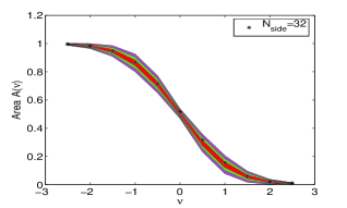
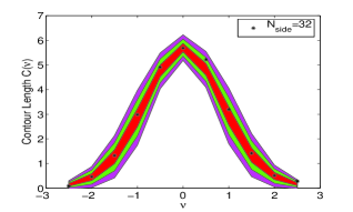
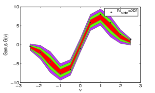
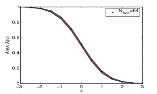
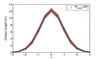
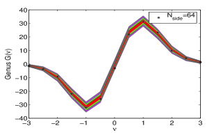
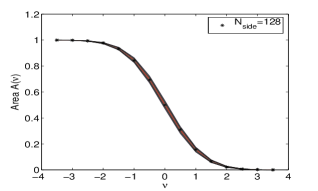
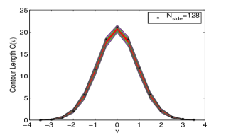
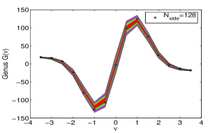
For this analysis we apply the statistical methods described in Sect. 3 to the Archeops 143K03 bolometer data. Figure 4 shows the Minkowski functionals as a function of threshold for maps with $N_{side}=32$, $N_{side}=64$, and $N_{side}=128$. In addition, we plot the acceptance intervals for the 68% (inner), the 95% (middle), and 99% (outer) significance levels obtained from 10000 noise and signal Gaussian simulations of the Archeops 143K03 data as described in Sect. 2. For all the analysed cases the data are compatible with Gaussianity at least at the 99% significance level.

In Fig. 5 we present the results of the Gaussianity analysis of the Archeops 143K03 bolometer data at different resolutions using the $\chi^{2}$ test described by Eqs. 5 and 11. In particular, we analysed the data at $N_{side}=32$ (11 thresholds, 3 functionals), $N_{side}=64$ (13 thresholds, 3 functionals), $N_{side}=128$ (15 thresholds, 3 functionals), the combination of the data at $N_{side}=32$ and $N_{side}=64$ (total of 24 thresholds, 3 functionals), and the combination of the data at $N_{side}=32$, $N_{side}=64$, and $N_{side}=128$ (total of 39 thresholds, 3 functionals). To avoid confusion by the non-Gaussianity of the Archeops noise at high resolutions, the high noise pixels were excluded as discussed in the previous Section. The histograms in the plot correspond to the analysis of 2000 Archeops signal plus noise Gaussian simulations at each resolution, the solid lines correspond to the expected $\chi_{3N_{th}}^{2}$ distribution, and the vertical lines correspond to $\chi^{2}$ values of the data at each resolution. For all the resolutions and combination of resolutions, the Archeops data are consistent with Gaussianity as expected from the previous figure. In Table 1 we present the $\chi^{2}$ value of the data for the different cases that we have analysed, the total number of degrees of freedom, the mean and the dispersion of the $\chi^{2}$ value of the Gaussian simulations, and the cumulative probability of the data computed from the distribution given by the simulations.

If we use all the available area at $N_{side}=128$ we find that Archeops data are not compatible with Gaussianity. In particular, we have obtained $P(\chi^{2}\leq\chi_{data}^{2})=0.995$ analysing the data at $N_{side}=128$, and $P(\chi^{2}\leq\chi_{data}^{2})=0.994$ analysing the data at $N_{side}=32,64,128$. These non-Gaussian deviations can be clearly associated with the non-Gaussianity of the Archeops noise at high resolution due to highly noisy pixels.

5.2 Constraints on $f_{nl}$ for realistic non-Gaussian simulations

The constraints in the $f_{nl}$ parameter were obtained using 300 CMB non-Gaussian simulations such as the one described in Sect. 2.3. and applying to the Archeops 143K03 bolometer data the $\chi^{2}$ test in the case of non-Gaussian fluctuations defined by an $f_{nl}$ parameter (Eq. 9). We computed an Archeops TOI for each realization and from it we computed the corresponding Mirage Archeops simulation for the $143K03$ bolometer. We did this for the Gaussian and non-Gaussian part separately. So we have

$$d_{k03}(f_{nl})=s_{g,k03}+f_{nl}*s_{ng,k03}+n_{g,k03}$$ (15)

where $s_{g,K03}$ is a Gaussian CMB simulation, $s_{ng,K03}$ is its corresponding non-Gaussian part, and $n_{g,K03}$ is a Gaussian instrumental noise simulation.

We computed the mean value of the Minkowki functionals, $\langle V\rangle_{f_{nl}}$, for $-1500\leq f_{nl}\leq 1500$. We assumed that in this interval the covariance matrix associated with them was dominated by the Gaussian contribution: i.e. $C_{ij}(f_{nl})\simeq C_{ij}(f_{nl}=0)$. Therefore, it was computed from $10^{4}$ Gaussian simulations of signal and noise ($s_{g,k03}+n_{g,k03}$) of the Archeops 143K03 bolometer. We obtained the $\chi^{2}(f_{nl})$ of Archeops data given by Eqs. 9 and 12 for the same combination of resolutions as the ones described in the above Gaussianity analysis. In all cases we find the value of $f_{nl}$ that minimizes $\chi^{2}(f_{nl})$. This is the best-fit value for the $f_{nl}$ parameter. The significance of these values is estimated using 2000 Gaussian simulations. For each simulation we computed $\chi^{2}(f_{nl})$ vs $f_{nl}$ and obtained its best fit $f_{nl}$. At the end we have a set of 2000 values of this parameter. As the simulations are Gaussian, these values are centred around $f_{nl}=0$.

Table 2 lists the best-fit $f_{nl}$ to the data for each case analysed. We also present the main properties of the distribution of the $f_{nl}$ parameter as obtained from the simulations. The smaller dispersion corresponds to the case where we combine the data at the three resolutions $N_{side}=$32, 64, and 128 (only 32% of the available area). Therefore this case leads to the best constraints of $f_{nl}$ for the Archeops data. In Fig. 6 we present the $\chi^{2}(f_{nl})$ vs $f_{nl}$ of the Archeops data and the histogram of the best fit $f_{nl}$ obtained from 2000 Gaussian simulations for this optimal case. From this we conclude that $f_{nl}=70_{-400}^{+590}$ at 68% CL and $f_{nl}=70_{-920}^{+1075}$ at 95% CL.

We may wonder if the constraints on the $f_{nl}$ parameter could be improved by increasing the area at $N_{side}=128$. We have shown that, if the noise were Gaussian, including the whole area available would have produced very similar constraints. The reason is that the excluded pixels were the noisiest ones and therefore increasing the area would not improve the results.

5.3 Comparing with the Sachs-Wolfe approximation

Table 3: Best fit of Sachs-Wolfe $f_{nl}$ of Archeops data at different resolutions, mean, dispersion and some percentiles.

Resolution	Area (%)	Best Fit $f_{nl}$	$\langle f_{nl}\rangle$	$\sqrt{\langle f_{nl}^{2}\rangle-\langle f_{nl}\rangle^{2}}$	$X_{0.160}$	$X_{0.840}$	$X_{0.025}$	$X_{0.975}$
32	100	-150	33	418	-375	425	-800	875
64	100	400	-3	252	-250	250	-500	500
128	32	-175	10	232	-225	250	-450	450
32,64	100,100	200	10	233	-225	250	-450	500
32,64,128	100,100,32	25	8	170	-175	175	-325	350

Figure 7: From left to right, the non-Gaussian part of a full sky CMB simulation at low resolution ($N_{side}=16$) and the corresponding Sachs-Wolfe quadratic approximation.

On large angular scales the main contribution to the CMB anisotropies is given by the Sachs Wolfe effect: $\Delta T/T=-\phi/3$ (Sachs & Wolfe 1967; Komatsu & Spergel 2001), where $\phi$ is the primordial potential. Therefore, in this case, the temperature map can be approximated in terms of a linear and a non-linear contribution in the following simple way:

$$\frac{\Delta T}{T}=\frac{\Delta T_{L}}{T}-3f_{nl}\left(\frac{\Delta T_{L}^{2}}{T^{2}}-\left\langle\frac{\Delta T_{L}}{T}\right\rangle^{2}\right)$$ (16)

where $\Delta T_{L}$ is Gaussian. We call this the Sachs-Wolfe approximation and to avoid confusion hereafter the $f_{nl}$ parameter in this case is called $f_{nl}^{SW}$. This approximation has been used in several works (for example Cayón et al. 2003a; Curto et al. 2007; Jeong & Smoot 2007). For this approximation the Archeops non-Gaussian simulations can be obtained as follows

$$d_{k03}(f_{nl})=s_{g,k03}-\frac{3f_{nl}^{SW}}{T_{0}}(s_{g,k03}^{2}-\langle s_{g,k03}^{2}\rangle)+n_{g,k03},$$ (17)

where $s_{g,k03}$ and $n_{g,k03}$ are Gaussian CMB and noise simulations respectively. As discussed above, this approximation is only valid for angular resolutions of a few degrees (Komatsu & Spergel 2001). Nevertheless we performed the non-Gaussianity analysis of the Archeops data at all considered scales in order to constrain $f_{nl}^{SW}$ and then tested the validity of this approximation as a function of the scale. In Table 3 we present the results of this analysis. We can see that for all the considered resolutions, the $f_{nl}$ constraints are better than for the case with the realistic simulations. This difference becomes more important as the resolution increases. The best constraints on $f_{nl}$ in this case are $f_{nl}^{SW}=25_{-150}^{+200}$ at 68% CL and $f_{nl}^{SW}=25_{-300}^{+375}$ at 95% CL using the combination of the data at $N_{side}=$ 32, 64 , and 128 (only 32% of the available area).

In general the Sachs-Wolfe approximation overestimates the non-Gaussianity of the CMB fluctuations for a given $f_{nl}$ value. This can be clearly seen in Fig. 7 where we present from left to right the histogram of the non-Gaussian part of a full sky CMB realistic simulation $\Delta T_{NG}$ and the corresponding quadratic approximation $-3f_{nl}/T_{0}(\Delta T_{G}^{2}-\langle\Delta T_{G}\rangle^{2})$ at resolution $N_{side}=16$ i.e. a pixel size of 3.6 degrees. We can see that even at this scale the simulations are very different. The approximation is just the square of a Gaussian distribution centred to have zero mean whereas the exact simulation is more Gaussian-like. This explains why the constraints on the $f_{nl}$ parameters are tighter for the Sachs-Wolfe approximation than for the exact case. Therefore, the results obtained with the Sachs-Wolfe approximation should be taken with caution, since the error bars are clearly underestimated.

6 Conclusions

In this paper we have presented a complete non-Gaussianity analysis of the Archeops data at 143 GHz using the Minkowski functionals. First, we characterised the Archeops instrumental noise by taking the difference of the data of the two most sensitive bolometers, 143K03 and 143K04. From this we found non-Gaussian deviations at high resolution, 27 arcmin ($N_{side}=128$ in the Healpix pixelization scheme). This is due to the noisiest pixels for which at high resolution the number of observations per pixel does not allow good systematic error removal. A more detailed analysis has been performed for the $143K03$ bolometer for which a noise map was obtained by subtracting the WMAP CMB data. From this analysis we found that pixels with a number of observations below 90 were non-Gaussian. Masking out those pixels, the noise map is compatible with a Gaussian model. Similar results were obtained with the $143K04$ bolometer although the minimum number of observations per pixel for Gaussianity was of the order of 150 and was not considered for further analysis.

Second, masking out these highly noisy pixels we performed a Gaussianity analysis of the Archeops $143K03$ data at low and high resolution. We found that the data are compatible with Gaussianity at $N_{side}=32$, $N_{side}=64$, $N_{side}=128$, and for the combinations $N_{side}=32,64$, and for the combinations $N_{side}=32,64,128$ at better than 95% CL. From this analysis and using realistic non-Gaussian simulations (Liguori et al. (2003)) we imposed constraints on the $f_{nl}$ parameter at these resolutions. The tightest constraints are $f_{nl}=70_{-400}^{+590}$ at 68% CL and $f_{nl}=70_{-920}^{+1075}$ at 95% CL.

Third, we also imposed constraints on $f_{nl}$ using the Sachs-Wolfe approximation, $f_{nl}^{SW}=25_{-150}^{+200}$ at 68% CL and $f_{nl}^{SW}=25_{-300}^{+375}$ at 95% CL. For comparison notice that these constraints are a factor of $\approx 3$ smaller than those given in Curto et al. (2007) where only low resolution ($N_{side}=32$) maps were considered.

Finally, we performed a detailed comparison of the realistic non-Gaussian simulations used in this paper and those from the Sachs-Wolfe approximation. From this we conclude that even at low resolution the Sachs-Wolfe approximation overestimates the non-Gaussianity of the CMB fluctuations and therefore the $f_{nl}$ constraints imposed are too tight by a factor of three, as shown above.