Elastic contact between self-affine surfaces: Comparison of numerical stress and contact correlation functions with analytic predictions
Abstract
Contact between an elastic manifold and a rigid substrate with a self-affine fractal surface is reinvestigated with Green’s function molecular dynamics. The Fourier transforms of the stress and contact autocorrelation functions (ACFs) are found to decrease as where is the wavevector. Upper and lower bounds on the ratio of the two correlation functions are used to argue that they have the same scaling exponent . Analysis of numerical results gives , where is the Hurst roughness exponent. This is consistent with Persson’s contact mechanics theory, while asperity models give . The effect of increasing the range of interactions from a hard sphere repulsion to exponential decay is analyzed. Results for exponential interactions are accurately described by recent systematic corrections to Persson’s theory. The relation between the area of simply connected contact patches and the normal force is also studied. Below a threshold size the contact area and force are consistent with Hertzian contact mechanics, while area and force are linearly related in larger contact patches.
pacs:
81.40.Pq,46.55.+dI Introduction
The distribution of pressures in the contact between two solids has a crucial influence on the amount of friction and wear that occur when the solids slide against each other. As a consequence, there is great interest in reliable predictions for the dependence of the distribution on the externally imposed load , the mechanical properties of the solids in contact, and their surface topographies [1]. Of course, it would be desirable to have theories at hand that allow one to calculate these distributions analytically or numerically at a moderate amount of computing effort. While solving numerically the full elastic or plasto-elastic behavior of contacting solids has become an alternative to studying analytical theories, numerically exact approaches incorporating long-range elastic deformation remain challenging to pursue. 111 Here, we wish to remind the reader that the term “numerically-exact method” stands for a numerical method, in which a model, such as an elastic manifold pressed against a corrugated wall with hard-wall repulsion, is solved in such a way that all systematic errors can be controlled, e.g., by the number of mesh points. In contrast, the GW and Persson approaches make uncontrolled approximations. This is because treating the wide range of length scales present in most surface topographies places great demands on computing time and memory.
Traditionally, many contact mechanics predictions were based on models following Greenwood and Williamson’s (GW) seminal paper [2], in which the contact between two solids is treated as the sum of non-interacting, single-asperity contacts. The crucial, geometric properties entering such theories are the statistics for asperity height and curvature. One of the most detailed treatments is by Bush et al. [3] who included a distribution of curvatures and elliptical asperities. In the last decade, Persson and collaborators have pursued a different approach [4, 5, 6, 7], in which the height autocorrelation function (ACF) is the geometric property that determines the pressure distribution and thereby the area of contact.
A central quantity in both GW and Persson’s theory is the ratio of the real area of microscopic contact to the macroscopic projected area of the surfaces . In the limit of low loads, both theories find that
| (1) |
where is a dimensionless constant of proportionality, is the mean pressure normal to the interface, is the root mean-square gradient of the height profile , and the effective elastic modulus , where is the Young’s modulus and the Poisson ratio. The generalization of GW by Bush et al. [3] predicts , while Persson theory yields . Numerically exact calculations for the relative contact area for solids with a self-affine surface topography are, give or take, half way between the two theoretical predictions [8, 9, 10].
Persson’s theory also provides a prediction for the functional dependence of the stress distribution , which can be described as the sum of a Gaussian of width centered at the macroscopic pressure and a mirror Gaussian centered at :
| (2) |
A -function contribution is added to so that the integral over from to yields unity. The prefactor to this -function contribution (divided by the normal macroscopic stress) can be interpreted as the relative area of the projected surface that is not in contact with the counterface. For the relevant non-negative pressures, the superposition leads to for small and Gaussian tails at large . GW theory gives distributions with similar limiting behavior. Numerical solutions for are qualitatively consistent with Eq. 2 when the parabolic peaks of asperities are resolved [9, 10], but some quantitative discrepancies remain as illustrated in the next section.
GW-type theories and Persson theory give quite distinct predictions for the spatial distribution of contact and pressure. Contact in GW is based on overlap of undeformed surfaces. This allows one to relate the contact ACF, , to the surface topography. gives the probability of finding contact at a coordinate if there is contact at a coordinate that is located at a distance away. In contrast, Persson’s theory contains a prediction for the stress ACF, . Both GW and Persson theory predict power law scaling for the correlation functions, but with very different exponents. In a numerically exact calculation, Hyun and Robbins found that and appear to decrease algebraically with in such a way that the two functions are essentially proportional to one another [10]. The values for the exponents that describe the decay of the autocorrelation functions were again found to be, give or take, half way between the theories. However, due to computational limitations, the uncertainty on the exponents was relatively large and only was studied.
Here, we would like to reassess these correlation functions with Green’s function molecular dynamics (GFMD) [11], which allows one to address larger system sizes than with finite-element methods or multiscale approaches [12]. One of our main goals in these calculations is to assess whether the relatively precise values of predicted by GW and Persson theory are to a certain degree fortuitous or if the theories also predict other computable observables, specifically stress and contact ACFs, with similar accuracy, i.e. of order twenty percent. We derive approximate and exact bounds on the ratio of these ACFs and their integrals that supplement the numerical results. The work presented here also includes a test of the claim that corrections to Persson’s theory can be derived with the help of a systematic expansion scheme derived recently by one of us [13]. The expansion has so far only been worked out (to harmonic order) for walls that repel each other with forces that increase exponentially when the distance between the surfaces decreases. Therefore, we also include comparison to numerically exact simulations based on exponentially repulsive walls. Finally, we conduct an analysis of connected contact patches for hard wall interactions to see if these regions show the characteristic behavior of Hertzian contact mechanics, as one would expect according to an overlap theory of purely repulsive, corrugated walls.
II Method
In this work, we model elastic, frictionless contact between two solids with self-affine surfaces. Use is made of the mapping of such a system onto contact between a flat elastically-deformable solid and a rigid, corrugated substrate [14]. The Green’s function molecular dynamics (GFMD) method [11] was used to solve for the elastic response of the deformable solid. Details of this method are provided in Ref. [11] and we only give the parameters of the model here. We chose both Lamé constants to be unity, which is equivalent to a Young’s modulus of , a bulk modulus of , and a Poisson ratio of . In what follows, most stated quantities will be dimensionless, but we take the Lamé constants as our unit of pressure. The continuum equations have no intrinsic length scale, so we will normalize lengths by the lateral resolution of the GFMD.
The surface topography of the rigid substrate was a self-affine fractal. Surfaces with the desired value of the Hurst roughness exponent were created using a Gaussian filter technique for the Fourier components of the height profile [15]. The long wavelength cutoff of fractal scaling is always identical to the length of our periodic simulation cell in both lateral directions. The effect of reducing is discussed in Ref. [10]. Unless noted . The effective depth of the deformable solid is also equal to . The short wavelength cutoff was varied from to . The wavevectors associated with the cutoffs and resolution are denoted as , , and . The magnitude of the Fourier components was adjusted to maintain the same mean-square height gradient for all and .
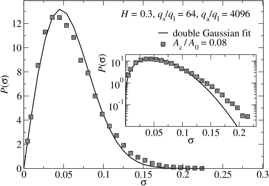
A wide range of parameters was considered. The roughness exponent was varied from 0.3 to 0.8, which covers the range of values typically reported in experiments [16, 17, 18, 19]. The load was varied between and , resulting in fractional contact areas between and . For each case we evaluated the spatial variation of the contact pressure . Then the total contact area , probability distribution of local pressures, and contact and pressure correlation functions were calculated. Since enters the analysis below, we show typical results in Figure 1, along with the analytic expression of Eq. 2. For this case , implying that the top of each asperity is resolved into a smooth parabolic peak. As a result, drops as decreases to zero. Extending the roughness to changes the form of at large and small , but does not change the power law behavior of the correlation functions at small that are our focus here [10].
The contact ACF, , is defined as
| (3) |
where and is the normal component of the stress at position . 222Note that is calculated from the force from the rigid substrate normalized by the area, , per ”atom” in the GFMD. Our calculation actually uses the component of this force which differs from the normal component by a factor of the cosine of the angle between the surface normal and the z-axis. Since the rms slope is only 0.031, the difference is negligible. The Heaviside step function, , is zero for negative and unity for positive arguments. However, unlike the usual convention, we choose , i.e., the step function is unity only at those locations where there is contact. The stress ACF is similarly defined as:
| (4) |
The ACF are most conveniently calculated by Fourier transforming. We choose the normalization so that
| (5) |
III Results
III.1 Relation between contact and stress autocorrelation functions
Traditional models ignore correlations in surface displacement due to elastic deformation so that the location of contacting regions is determined solely by the local height. We will refer to such models generically as ”overlap models”. A particular overlap model is the bearing area model [14] in which contact occurs wherever the undeformed solids would overlap. For the case of rough on flat considered in our calculations, this corresponds to the region where the height of the rough solid is above a threshold value. In the GW model and extensions [2, 3], the same criterion is used to determine which asperities are in contact, and the corresponding load is obtained from the force needed to remove overlap. Since contact only depends on the local height in such models, it is relatively easy to construct the contact morphology for any given surface topography. One can then calculate the relative contact area and .
Since the location of contacts is entirely determined by the height in the bearing area and GW model, Hyun and Robbins argued that should have the same scaling as the height-height correlation [10, 15]:
| (6) |
Their numerical results for were consistent with this relation. We are not aware of any specific predictions for the stress ACF in the GW model, although it might also follow since the stress on asperities is also determined directly by their height.
In contrast, Persson’s scaling theory does not consider , but contains implicit predictions for the stress ACF. In the limit of complete contact, Persson theory becomes exact. The stress correlation function can be determined from the height correlation function and the elastic Greens function. The latter scales as , yielding [20]. This result is consistent with numerical studies of full contact [21]. The original version of Persson theory does not discuss stress ACFs in partial contact explicitly. One may thus be tempted to use the full contact approximation for the stress ACF at all loads. However, when contact is not complete, only a fraction of the elastic manifold conforms to the counterface and so the full contact ACF only provides an upper bound, as the non-conforming parts of the manifold do not carry any load. After receiving a preprint of our work, Persson informed us that a correction factor needs to be included into the calculation to capture this effect [22]. This correction factor is the relative contact area at a given “magnification”, i.e., one needs to correct with the relative contact area that his theory would predict if all roughness for wavevectors of magnitude greater than were eliminated. (This correction factor had already been introduced for the calculation of adhesive interactions in earlier work[5].) With this correction factor the exponent is obtained in Persson theory for partial contact. In particular,
| (7) |
where the first term is the full contact prediction and [5, 22].
While the power laws in Equations 6 and 7 are very different, it is not clear how the scaling of the stress ACF and contact ACF should be related. In the following we argue that two approximate bounds on the ACF’s force them to have the same scaling exponents. In particular,
| (8) |
where and are the mean and second moments of the stress averaged over those areas where there is contact, i.e.,
| (9) |
In cases where the stress histogram, can be described by equation (2), one can easily find that . The same ratio is obtained for the approximately exponential distribution of pressures found for surfaces with [8]. Similar ratios are obtained for the other considered here, leading us to add the approximate equality at the right of Eq. 8.
In the limit , the stress ACF is exactly equal to the upper limit of Eq. 8: . In the large limit, the local values of the stress should become decorrelated, and will then equal the lower limit. One expects a smooth crossover between the two bounds as increases unless there is a strong correlation at some given wavelength. For example, one can construct counterexamples to the bounds such as a perfectly sinusoidal surface topography.
Figure 2 presents typical numerical results for the ACF’s of self-affine surfaces. Values of lie close to the upper bound up to , and then cross over rapidly to the lower bound. A heuristic reason for the more rapid drop in than can be constructed as follows. Consider the contribution to these two ACFs that stem from two points and that are in the same contact patch, for example, within a single Hertzian contact. The contribution to will simply be unity, i.e., cannot decay within a simply-connected contact region. Conversely, can and will have a lot of structure, e.g., the correlation between the stress at the center and edge of a Hertzian contact will be small. Consequently, a significant fraction of will have decayed on a length-scale that is comparable to a typical contact radius, while only a very small fraction of will have decayed on that same distance. Note that the rapid decay in Fig. 2 starts at which should be comparable to the smallest contacts. Since contacts of many different sizes are found, one may conjecture that falls off faster than for all . The difference should decrease at large as the number of connected clusters with dimension greater than decreases.
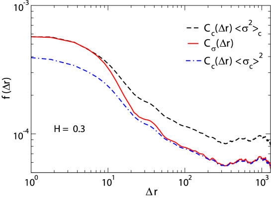
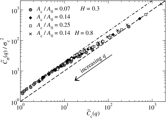
Fig 3 illustrates that the same upper and lower bounds describe the Fourier transforms of the correlation functions. Data for a range of and relative areas are shown. In each case there is a crossover from the lower bound of Eq. 8 at small (large ) to the upper bound at large .
One can derive additional relations for the Fourier transforms of the ACF’s that support the bounds quoted above. First, the values must obey:
| (10) | |||||
| (11) |
where is the number of (or real-space grid points) in the sum. This shows that in the limit the correlation functions satisfy the lower bound in Eq. 8. One can also use a general sum rule over real and reciprocal space to write:
| (12) |
and similarly
| (13) |
The last two equations show that the sum over all of the ACFs is exactly consistent with the upper bound in Eq. 8. While this implies that the upper bound must be exceeded for some , we will see that the sum is dominated by large where the upper bound is nearly obeyed. Our focus is on the power law scaling regime in the opposite limit of small .
In order to collapse data for different loads it is useful to recast the above sum rules. It is also helpful to eliminate the term since we will see that the ACFs diverge in the limit . In addition, the term scales as , while other terms scale linearly with . Subtracting Eq. 11 from Eq. 13 and rearranging factors we find:
| (14) |
where . We will see that scaling in this way removes the dependence on at small . Evaluating the same weighted sum for the stress ACF yields
| (15) |
Using the same scaling of the two ACF’s guarantees that they coincide as . While will decay more slowly at large , the fact that its integral over all is larger by only a factor of order 2 for any system size implies that should be described by the same scaling exponent as .
III.2 Comparison to overlap theories
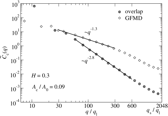
Figure 4 compares results for from the full GFMD calculation and the GW model which uses overlap to determine contact. Both models yield roughly power law behavior at intermediate
| (16) |
However there is a large discrepancy in the numerical values between GFMD () and the bearing area model (), which one can conclude from figure 4. A similar difference in the values for is observed for other and , as reported for in Ref. [10]. There is a simple physical reason that overlap models yield larger and thus cluster the contact patches too closely. They neglect the fact that an asperity in the vicinity of a very high asperity is less likely to come into contact because it is pushed down when that very high asperity comes in contact with the counter-surface [6, 8, 10, 23].
In all cases, our numerically determined exponent for the bearing area model is consistent with the estimate , within our uncertainty of for this model. In contrast, the GFMD results are consistent with within an uncertainty of . The reason for the difference in the uncertainties of our estimates stems from the fact that contact geometries associated with large have large finite-size effects, particularly when exceeds two. 333 We found was 3.1 for and 2.8 for for the bearing area model, while the size effect was merely 0.1 for the GFMD data. This is because a large value of implies significant contributions from long wavelengths, which have less sampling than short wavelengths, as can be seen from an analysis of :
| (17) | |||||
| (18) |
For the contribution at small is finite. One can change the integration variable to and finds:
| (19) |
at large with . This is the type of behavior we find for our numerical solutions, i.e. Fig. 2.
The behavior becomes qualitatively different if as predicted by the relation for the bearing area model. This implies a singular contribution from small in Eq. 18 and suggests that should increase with . The origin of this behavior seems to be related to the distribution of sizes of connected regions in the bearing area model. The probability that a cluster will have area is predicted [15] to scale as with . Since , most of the contact area is in the clusters of largest size, and there will be no decay in on this scale. The dominance of large clusters leads to significant fluctuations in data for the bearing area model that are not seen in the numerical solution with GFMD. We conclude that the bearing area model and thus GW provide a very poor description of the contact ACF.
III.3 Numerical Determination of
To determine accurate values of the scaling exponents describing the ACF’s we maximized the scaling region by taking . Our results and earlier work [10] show that resolving the asperities is not important to the large scale behavior of interest here. Figure 5 shows results for and at , and . In each case, data for two different area fractions, corresponding to about 4% and 8% have been collapsed by plotting following Eq. 14. With this rescaling, the data for the two loads are indistinguishable. This is consistent with previous numerical work that indicates area fractions of less than 10% exhibit scaling behavior consistent with the asymptotic small limit [8, 10, 23].
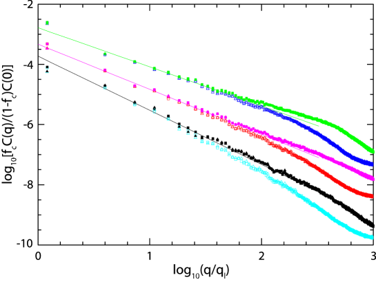
At small the stress and contact ACF follow the same scaling. Straight lines show that the data are consistent with in this regime. This ansatz for the scaling exponent was motivated by the fact that is bigger than the value predicted for full contact by an amount that decreases with increasing (see below). It also ensures that remains below 2 as increases to unity, and thus that the real space correlation function has nonsingular scaling behavior. If both stress and contact ACF are assumed to have the same exponent in numerical fits to the data, then the deviation from is less than 0.1 (Table 1). However, the fact that always decays by about an extra factor of two means that separate fits always give . Given that our scaling range is only a decade and a half, the magnitude of this difference is of order . We cannot rule out deviations between and on this scale and it represents the major source of uncertainty in Table 1. Given this uncertainty, it is possible that may reach or exceed 2 before reaches unity. As for overlap models, this would imply singular contributions from large contacts, and anomalous behavior of the correlation function at large .
| GFMD | GW | Persson | |
|---|---|---|---|
III.4 Comparison to Persson theory
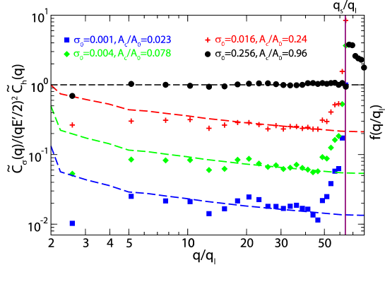
When comparing the GFMD results to Persson’s theory, it is more convenient to compare the stress ACFs rather than the contact ACFs. Figures 6 and 7 show our numerical results for normalized by the stress ACF from the full contact approximation ( in Eq. 7). Results are shown for a wide range of loads that give relative contact area between 2% and 96%. Note that theory and simulation should not be compared for where and the plotted ratio is not well defined.
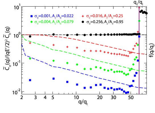
Our numerical results for are nearly indistinguishable from the full contact expression. As decreases, the discrepancies from full contact increase. The magnitude of is depressed and the data drop with an apparent power law indicating that . The deviation is clearly smaller for than , but is present in both cases.
In Persson’s theory with corrections for partial contact (Eq. 7) the ratio plotted in Figs. 6 and 7 should equal , the relative contact area for surfaces resolved to [5, 22]. Dashed lines in the figures plot the numerically determined for the same surfaces. For smaller relative contact area, the theory still captures the trend correctly, i.e., the power laws with which the ACFs decay at large are very similar to the numerical data. The theoretical prefactors are generally better for large than for small , which is consistent with the observation that the value for predicted by Persson improves with increasing [8].
For a few of the largest area fractions (not included here to make the figures clear), there appears to be a crossover at a wave vector . For the results converge to the full contact prediction, while for the results follow the larger exponent observed at small area fractions. It is intriguing to note that the crossover behavior is observed in the simulations only near and above the percolation probability for a square lattice [24]. This suggests that when the contacting area percolates, the system behaves as if it were in full contact at large scales. The wavelength corresponding to might then correspond to the size of the largest non-contacting regions, leading to an increase in as the area fraction increases. Tests of these conjectures are beyond the scope of this work.
III.5 Comparison to field-theoretical approach
In reference [13], it was argued by one of us (MHM) that Persson’s theory corresponds to the leading-order term of a rigorous field-theoretical expansion. The expansion is formally based on the assumption that a (free) energy functional exists describing the interaction between two contacting solids, which depends on the gap separating the two solids.
For exponential repulsion, corrections to Persson’s theory were worked out explicitly up to harmonic order. The main result relevant for the calculation of the correlation function is that equation (7), which is valid in Persson’s theory, will be replaced with
| (20) |
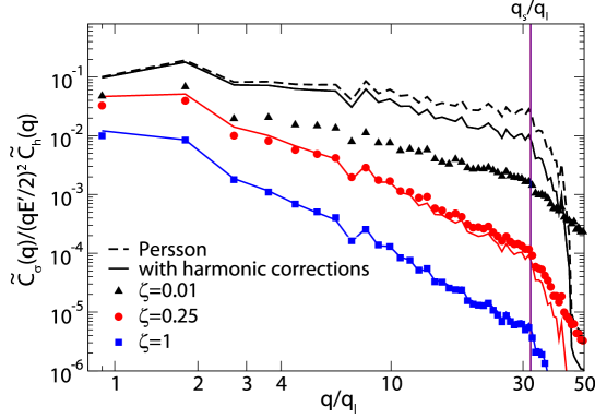
Here, is a correction factor that depends on the characteristic screening length of the exponential repulsion, the magnitude of the wavevector, the effective elastic constant and the macroscopic normal stress . As the normal force is never exactly zero, we have used for all values of in the evaluation of Eq. (7). Thus, like Persson theory, the field theory has no adjustable coefficient. In the limit , corrections disappear.
In figure 8 comparison is made between numerical results and the field theory. The numerical data was based on the same calculations as those presented in reference [13]. It can be seen that corrections to Persson theory are very small for the smallest value of the screening length analyzed here, i.e., for . However, for a value of the agreement between predicted and calculated stress ACF is essentially perfect for the relevant wave vectors. The degree of agreement is surprisingly good, given the relatively poor agreement in the stress histograms for that same value, see figure 1 in reference [13]. At the largest value of , that is, , there is almost perfect agreement, as to be expected for a rigorous expansion that is most accurate for large values of .
III.6 Analysis of connected contact patches
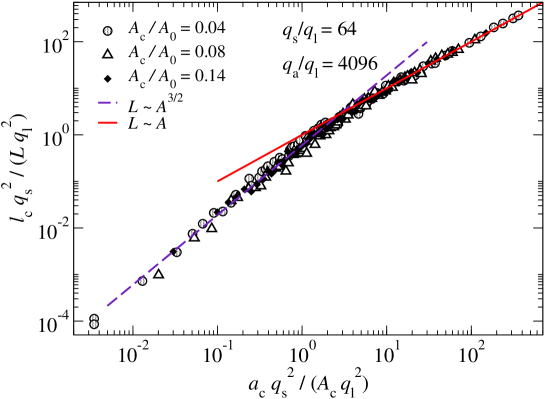
A merit of GW and related theories is that they provide an intuitive explanation for why total load and true area of contact are proportional to one another at small loads and thus that is constant. Although the relation between area and local load for any individual contact is non-linear in these theories, , the number of contacts of each area rises linearly with load. As the total load increases, a contact that already exists will have an increased local load and grow in size. However, new contacts will form under increasing so that there is a supply of new contact patches with small local loads. Under certain favorable conditions, the distribution of contact loads and sizes maintains the same shape and remains constant. Previous work shows that while the distribution of contact areas is different than the GW prediction, it is independent of load at small loads [8]. Here we examine the relation between load and area within these patches.
In figure 9 we present data for a number of systems with . In particular we analyze the load that connected contact patches carry as a function of their area . It can be seen that the data decomposes into two scaling regimes. At small , the data follow the prediction of Hertzian contact mechanics that is used in GW, . At large , the load exhibits the linear scaling with area that is found for the entire macroscopic contact area. The crossover occurs when the contact area is comparable to the square of the small wavelength cutoff in the fractal scaling. At smaller scales single asperities are fully resolved, while at larger scales one sees the effects of roughness with many wavelengths. GW theory does not include the effect of these larger scales and it is interesting that the linear scaling of area and load enters so close to . Hyun and Robbins have shown that there is also a crossover in the the probability of finding clusters of a given size at . The probability is nearly flat for and falls off as a power law at larger .
IV Discussion and Conclusions
In this work, we computed the stress and contact ACFs that one obtains when pressing an elastically deformable solid against a rough, rigid, non-adhesive, and impenetrable substrate. Analytic arguments were presented for approximate bounds and exact sum rules on the stress and contact ACFs. These imply that decays more rapidly with wavevector than , but that the change in their ratio is only about a factor of two, no matter how large the system. As a result, the decrease of these ACFs with wavevector must be described by the same scaling exponent .
Numerical results for were compared to the predictions of analytic theories for roughness exponents that span the typical range for experimental surfaces (Table 1). Our GFMD results are consistent with within an error of 0.1. This is only half the value predicted by the bearing area and GW models, which neglect the elastic interactions between deforming asperities. Persson’s theory includes these correlations through an approximation for the stress ACF that becomes exact in the limit of full contact. Recent extensions of his model[5, 22] that include corrections for partial contact lead to a scaling exponent that is consistent with our numerical data [22]. The prefactor predicted by this model appears to be slightly too high at small , but to approach the numerical results as . This is also the limit where the assumption of full contact is most accurate. In this context it is interesting to note that the value of (Eq. 1) also seemed to approach Persson’s prediction as in earlier work [8].
In this work we also tested whether a recently suggested field-theoretical approach to contact mechanics allows one to improve predictions for the stress ACFs [13]. The new approach can be interpreted as an expansion, in which the perturbation parameter is a screening length which describes the exponential repulsion between two surfaces. A zero screening length corresponds to hard wall interactions. In this limit the leading order term of the expansion reduces to Persson’s theory. Our numerical results suggest that including the next non-vanishing term vastly improves the agreement between calculated and predicted stress ACFs.
Lastly, analysis of the load that is carried by connected contact patches revealed a crossover at a critical patch size. Smaller contacts exhibit a Hertzian relation between area and load. Larger contacts exhibit a linear relation between area and load. This linearity at the contact scale may be part of the reason that a linear relation between area and load is observed for the entire surface.
Acknowledgments: MHM thanks Matt Davison for helpful discussions.
Computing time from SHARCNET as well as financial support from NSERC,
General Motors and National Science Foundation Grant No. DMR 0454947 are gratefully acknowledged.
References
- [1] F. P. Bowden and D. Tabor. Friction and Lubrication. Wiley, New York, 1956.
- [2] J. A. Greenwood and J. B. P. Williamson. Proc. R. Soc. London, A295:300, 1966.
- [3] A. W. Bush, R. D. Gibson, and T. R. Thomas. Wear, 35:87, 1975.
- [4] B. N. J. Persson. J. Chem. Phys., 115:3840, 2001.
- [5] B. N. J. Persson. Eur. J. Phys. E, 8:385, 2002.
- [6] B. N. J. Persson, F. Bucher, and B. Chiaia. Phys. Rev. B, 65:184106, 2002.
- [7] B. N. J. Persson, O. Albohr, U. Tartaglino, A. I. Volokitin, and E. Tosatti. J. Phys.: Condens. Matter, 17:R1, 2005.
- [8] S. Hyun, L. Pei, J.-F. Molinari, and M. O. Robbins. Phys. Rev. E, 70:026117, 2004.
- [9] C. Campañá and M. H. Müser. Europhys. Lett., 77:38005, 2007.
- [10] S. Hyun and M. O. Robbins. Tribol. Int., 40:1413, 2007.
- [11] C. Campañá and M. H. Müser. Phys. Rev. B, 74:075420, 2006.
- [12] C. Yang, U. Tartaglino, and B. N. J. Persson. Eur. J. Phys., 19:47, 2006.
- [13] M. H. Müser. Phys. Rev. Lett., 100:055504, 2008.
- [14] K. L. Johnson. Contact Mechanics. Cambridge University Press, Cambridge, 1966.
- [15] P. Meakin. Fractals, scaling and growth far from equilibrium. Cambridge University Press, New York, 1977.
- [16] D. Bonamy, L. Ponson, S. Prades, E. Bouchaud, and C. Guillot. Scaling exponents for fracture surfaces in homogeneous glass and glassy ceramics. Phys. Rev. Lett., 97:135504, 2006.
- [17] E. Bouchaud. Scaling properties of cracks. J. Phys. Conden. Matter, 9:4139–4344, 1997.
- [18] J. H. Dieterich and B. D. Kilgore. Imaging surface contacts: power law contact distributions and contact stresses in quartz, calcite, glass and acrylic plastic. Tectonophysics, 256:219–239, 1996.
- [19] J. Krim and G. Palasantzas. Experimental observation of self-affine scaling and kinetic roughening at sub-micron lengthscales. Int. J. of Modern Phys. B, 9:599–632, 1995.
- [20] J. A. Greenwood. Contact pressure fluctuations. J. Eng. Tribology, 210:281–284, 1996.
- [21] S. Roux, J. Schmittbuhl, J.-P. Vilotte, and A. Hansen. Some physical properties of self-affine surfaces. Europhys. Lett., 23:277–282, 1993.
- [22] B. N. J. Persson, private communication and arXiv:0805.0712v1 [cond-mat soft].
- [23] C. Campañá, M. H. Müser, C. Denniston, Y. Qi, and T. Perry. J. Appl. Phys., 102:113511, 2007.
- [24] D. Stauffer and A. Aharony. Introduction to Percolation Theory. Taylor and Francis, London, 2nd edition, 1971.