N-MODY: a code for collisionless N-body simulations in modified Newtonian dynamics

Abstract

We describe the numerical code N-MODY, a parallel particle-mesh code for collisionless N-body simulations in modified Newtonian dynamics (MOND). N-MODY is based on a numerical potential solver in spherical coordinates that solves the non-linear MOND field equation, and is ideally suited to simulate isolated stellar systems. N-MODY can be used also to compute the MOND potential of arbitrary static density distributions. A few applications of N-MODY indicate that some astrophysically relevant dynamical processes are profoundly different in MOND and in Newtonian gravity with dark matter.

1 Introduction

Modified Newtonian dynamics (MOND) is an alternative gravity theory, originally proposed by Milgrom (1983) to explain the observed kinematics of disk galaxies without dark matter. In Bekenstein & Milgrom’s Lagrangian formulation of MOND (Bekenstein & Milgrom 1984) the Poisson equation is replaced by the non-linear field equation

$$\nabla\cdot\left[\mu\left({\|\nabla\phi\|\over a_{0}}\right)\nabla\phi\right]=4\pi G\rho,$$ (1)

where $a_{0}\simeq 1.2\times 10^{-10}{\rm m\,s^{-2}}$ is a characteristic acceleration, $\|...\|$ is the standard Euclidean norm in $\mathbb{R}^{3}$, and $\phi$ is the MOND gravitational potential produced by the density distribution $\rho$. The MOND interpolating function $\mu(y)$ is a monotonic function such that

$$\mu(y)\sim\cases{y&for $y\ll 1$,\cr 1&for $y\gg 1$.}$$ (2)

For finite mass systems the boundary condition of equation (1) is $\nabla\phi\to 0$ for $\|{\bf x}\|\to\infty$.

As MOND is successful in reproducing several observed properties of galaxies (e.g. Bekenstein 2006), there is growing interest in studying dynamical processes in MOND with the aid of N-body simulations. While in Newtonian gravity N-body codes can take advantage of the multipole expansion of the Green function (treecodes; Barnes & Hut 1986; Dehnen 2002), the non-linearity of the MOND field equation forces one to solve for the potential on a grid, as done in particle-mesh schemes (see Hockney & Eastwood 1988).

We developed N-MODY, a parallel three-dimensional particle-mesh code for collisionless N-body simulations in MOND. The N-body code and the potential solver on which the code is based have been already tested and applied in Ciotti et al. (2006, 2007) and Nipoti et al. (2007a, b, c, 2008). The potential solver of N-MODY solves the MOND field equation (1) using a relaxation method in spherical coordinates based on the spherical harmonics expansion. Thus the code is ideally suited for simulations of isolated stellar systems (but see Nipoti et al. 2007c, for an application to galaxy merging). N-MODY can also be used to compute the MOND potential of arbitrary static density distributions. N-MODY is one of the very few MOND N-body code developed so far: as far as we know the only other three-dimensional MOND N-body code is Brada and Milgrom’s code (Brada & Milgrom 1999), which is based on a multi-grid potential solver in Cartesian coordinates and has been recently implemented also by Tiret & Combes (2007).

2 Overview of the code

N-MODY implements a particle-mesh scheme in spherical coordinates, following these main computational steps:

1. for a given distribution of $N$ particles, a grid-based density field is reconstructed by mass deposition with linear or quadratic shape functions. Particles are represented by a six-component array $({\bf x}_{p},{\bf v}_{p})$ of positions and velocities in Cartesian components ($p=1,...,N$).

2. For a given density distribution, the MOND acceleration and potential fields are computed on the grid points. As an alternative, the code also provides a fast Newtonian solver.

3. To move particles, the spherical components of the acceleration are first interpolated at each particle position (using the same linear or quadratic shape functions used in the mass deposition) and then transformed into Cartesian components.

4. Finally, particle positions and velocities are advanced in time using a leapfrog scheme of either second or fourth order.

In N-MODY steps 1) and 3) are parallelized using MPI routines: particles are uniformly distributed among the processors (PEs) following the sequential ordering provided by their initial memory addresses and then never exchanged among different PEs. This simple strategy assures a full efficiency in parallel execution, but entails more memory resources than in a standard domain decomposition. In fact, grid data computed on the overall computational domain must be at disposal of each PE at each timestep for particles interpolation and move. Step 2), which is only partially parallelized, contains the MOND potential solver, which represents a new contribution to the fast numerical solution of a non-linear elliptic equation. We now discuss in more detail the different parts of the code: the potential solver is described in Section 3, while the particle-mesh scheme and the time integration are described in Section 4.

3 The MOND potential solver

N-MODY solves the non-relativistic MOND field equation (1). By default in N-MODY we adopt as interpolating function $\mu(y)={y/\sqrt{1+y^{2}}}$, but it is clear that a trivial modification of the code allows to implement any other continuous function $\mu$ with the required asymptotic behaviour. N-MODY can also be used to simulate a Newtonian system, in which case the Poisson equation is solved instead of equation (1), or a system in the so-called ‘deep MOND regime’, i.e. obeying the equation $\nabla\cdot\left({\|\nabla\phi\|}\nabla\phi\right)=4\pi Ga_{0}\rho$.

We consider only systems of finite mass $M=\int\rho({\bf x})\,d^{3}{\bf x}$, for which the boundary conditions of equation (1) are given by $\|\nabla\phi\|\to O(1/r)$ for $r\equiv\|{\bf x}\|\to\infty$. It must be stressed that the asymptotic behaviour of the MOND potential ($\phi\sim\ln r\to\infty$ for $r\to\infty$) is profoundly different from that of the Newtonian potential ($\phi\to 0$ for $r\to\infty$). For this reason, to solve numerically the MOND field equation (i) we discretize a sufficiently large computational domain, in a way the asymptotic boundary condition can be represented with reasonable accuracy and (ii) we use a relaxation method to solve the non–linear elliptic equation (1) with guess solution having the correct asymptotic behaviour.

3.1 The computational grid

To accomplish task (i) above, N-MODY uses a spherical grid $(r,\vartheta,\varphi)$ with radial coordinate represented by the invertible mapping

$$r(\xi)=L\tan^{\alpha}\xi,\quad r^{\prime}(\xi)={\alpha L\tan^{\alpha-1}\xi\over\cos^{2}\xi},$$ (3)

where $0\leq\xi<\pi/2$, the mapping index $\alpha=1$ or $\alpha=2$ and the scale length $L$ are user provided parameters (see Londrillo & Messina 1990). In this representation, the unbounded radial range $(0,\infty)$ is mapped onto the finite open interval $[0,\pi/2)$. The radial derivative is then expressed as

$${\partial\over\partial r}={1\over r^{\prime}(\xi)}{\partial\over\partial\xi}$$ (4)

and the $\xi$ coordinate is discretized into the uniform grid

$$\xi_{i}=(i+1/2)\Delta\xi,\quad\Delta\xi={\pi\over 2N_{r}},\quad i=0,1,..,N_{r},$$ (5)

so the corresponding discretized radial variable $r_{i}=r(\xi_{i})$ avoids the singular points $r=0$ and $r=\infty$. The other coordinates $(\vartheta,\varphi)$ are discretized in the uniform grids

$$\vartheta_{j}=(j+1/2)\Delta_{\vartheta},\quad\Delta_{\vartheta}=\pi/N_{\vartheta},\quad j=0,1,..,N_{\vartheta}-1,$$ (6)

to avoid the singular points $\vartheta=0$ and $\vartheta=\pi$, and

$$\varphi_{k}=k\Delta_{\varphi},\quad\Delta_{\varphi}=2\pi/N_{\varphi},\quad k=0,1,..,N_{\varphi}-1.$$ (7)

The corresponding $(\xi,\vartheta,\varphi)$ numerical derivatives are computed by second-order or fourth-order finite difference central schemes.

3.2 A Newton-like relaxation procedure

In N-MODY we use a Newton-like relaxation procedure to solve the non–linear MOND equation, which can be written as

$$\hat{M}[\phi({\bf x})]\equiv\nabla\cdot\left[\mu\left({g\over a_{0}}\right)\nabla\phi({\bf x})\right]-4\pi G\rho({\bf x})=0,\quad g=O(r^{-1})\quad{\rm for}\quad r\to\infty,$$ (8)

where $\rho({\bf x})$ is assigned, $g({\bf x})=\|{\bf g}({\bf x})\|$, with ${\bf g}({\bf x})=-\nabla\phi({\bf x})$, and ${\bf x}=(r,\vartheta,\varphi)$. Starting with an approximate guess solution $\phi^{(0)}$ having the required asymptotic behaviour, a sequence of linear problems

$$\hat{R}^{(n)}\delta\phi^{(n)}=-\hat{M}\left[\phi^{(n)}\right],\quad n=0,1,...$$ (9)

is solved for the increments $\delta\phi^{(n)}=\phi^{(n+1)}-\phi^{(n)}$, each $\phi^{(n)}$ provisional solution having the same asymptotic behaviour as the guess $\phi^{(0)}$. Here the choice of the relaxation linear operator $\hat{R}^{(n)}$ is based on the requirement that it must assure convergence in the maximum norm $\|...\|_{\infty}$, i.e.

$$\left\|\delta\phi^{(n)}\right\|_{\infty}=\left\|\left[\hat{R}^{(n)}\right]^{-1}\hat{M}\left[\phi^{(n)}\right]\right\|_{\infty}\leq\left\|\delta\phi^{(n-1)}\right\|_{\infty},\quad n=1,2,...,$$ (10)

and it must be easy to invert. In a classical Newton method, one would use $\hat{R}^{(n)}=\delta\hat{M}^{(n)}$, where the linear operator $\delta\hat{M}^{(n)}$ is such that

$$\delta\hat{M}^{(n)}\left[\delta\phi^{(n)}\right]=\hat{M}\left[\phi^{(n+1)}\right]-\hat{M}\left[\phi^{(n)}\right]+O\left[(\delta\phi^{(n)})^{2}\right].$$ (11)

For the specific case of $\hat{M}$ defined by equation (8),

$$\delta\hat{M}^{(n)}=\mu^{(n)}\nabla^{2}+\delta\hat{M}^{(n)}_{1},$$ (12)

where

$$\delta\hat{M}^{(n)}_{1}=(\nabla\mu^{(n)})\cdot\nabla+\nabla\cdot\left[\mu^{\prime(n)}{\bf g}^{(n)}{\left({\bf g}^{(n)}\cdot\nabla\right)}\right]$$ (13)

and $\mu^{\prime(n)}\equiv\mu^{\prime}\left({g^{(n)}/a_{0}}\right)/g^{(n)}a_{0}$. Boundedness of the inverse of the operator $\delta\hat{M}^{(n)}$ assures quadratic convergence of the scheme for $\phi^{(0)}$ sufficiently close to the sought solution (e.g. Stoer & Bulirsch 1980). Unfortunately, $[\delta\hat{M}^{(n)}]^{-1}$ is difficult to compute, so we discretize the simpler linear operator

$$\hat{R}^{(n)}=\omega\mu^{(n)}\nabla^{2},$$ (14)

where $\omega>1$ is an empirical relaxation parameter. As an approximation of the Newton relaxation operator $\delta\hat{M}$, this choice assures a lower convergence rate, but has clear computational advantages. Using equation (9) and the identity

$$\hat{M}(\phi^{(n)})=\delta\hat{M}^{(n-1)}\left[\delta\phi^{(n-1)}\right]+\hat{M}\left[\phi^{(n-1)}\right]+O\left[(\delta\phi^{(n-1)})^{2}\right],$$ (15)

it follows that the condition for convergence (10) requires

$$\left\|{(\nabla^{2})^{-1}\delta\hat{M}^{(n-1)}\over\omega\mu^{(n)}}-{\mu^{(n-1)}\over\mu^{(n)}}I\right\|_{\infty}<1.$$ (16)

Thus N-MODY solves the sequence of Poisson equations:

$$\nabla^{2}\delta\phi^{(n)}={\mathcal{S}}^{(n)},\quad n=0,1,...,$$ (17)

with source term given by

$${\mathcal{S}}^{(n)}=-{1\over\omega\mu^{(n)}}\hat{M}\left[\phi^{(n)}\right].$$ (18)

In spherical coordinates, the Laplacian operator has the form

$$\nabla^{2}\equiv{1\over r^{2}}\left[{\partial\over\partial r}\left({r^{2}{\partial\over\partial r}}\right)+\hat{L}_{\vartheta}+\hat{L}_{\varphi}\right],$$ (19)

where

$$\hat{L}_{\vartheta}\equiv{1\over\sin\vartheta}{\partial\over\partial\vartheta}\left(\sin\vartheta{\partial\over\partial\vartheta}\right),\quad\hat{L}_{\varphi}\equiv{1\over\sin^{2}\vartheta}{\partial^{2}\over\partial\varphi^{2}}.$$ (20)

After expanding the unknown function $\delta\phi^{(n)}(r,\vartheta,\varphi)$ and the source term ${\mathcal{S}}^{(n)}(r,\vartheta,\varphi)$ in spherical harmonics (or Fourier-Legendre) components

$$\delta\phi^{(n)}(r,\vartheta,\varphi)=\sum_{l,m}\delta\phi_{l,m}^{(n)}(r)Y_{l}^{m}(\vartheta,\varphi),\quad{\mathcal{S}}^{(n)}(r,\vartheta,\varphi)=\sum_{l,m}{\mathcal{S}}_{l,m}^{(n)}(r)Y_{l}^{m}(\vartheta,\varphi),$$ (21)

equation (17) takes the simple one-dimensional form

$${1\over r}\left[{d\over dr}\left({r^{2}{d\over dr}}\right)-l(l+1)\right]\delta\phi_{l,m}^{(n)}(r)=r{\mathcal{S}}_{l,m}^{(n)}(r),$$ (22)

where we multiplied both sides by $r$ to avoid the singularity in the source term for the astrophysically relevant case of $\rho\sim r^{-1}$ central density profiles. Equation (22), involving derivatives only in the radial coordinates, is discretized by central finite differences.

3.3 Implementation of the relaxation procedure.

The relaxation scheme in N-MODY is implemented in the following steps:

1. At the initial time $t=0$ in N-body simulations (and in the case of static models) the guess solution $\phi^{(0)}$ is chosen to be the spherically symmetric MOND solution of the angle-averaged density distribution

   $$\rho_{0,0}(r)={1\over 4\pi}\int_{0}^{2\pi}\int_{0}^{\pi}\rho(r,\vartheta,\varphi)\sin\vartheta\,d\vartheta\,d\varphi,$$ (23)

   which is easily derived from the corresponding spherical Newtonian solution (Bekenstein & Milgrom 1984). In particular this guess solution satisfies the boundary condition, providing the values of the potential $\phi^{(0)}$ and of the radial acceleration $g_{r}^{(0)}$ at the boundary grid point $r_{N_{r}}$. At $t>0$ in N-body simulations the guess solution is provided by the numerical solution found in the previous timestep.

2. For assigned acceleration ${\bf g}^{(n)}(r,\vartheta,\varphi)$ at the iteration level $n$, the source term $r{\mathcal{S}}^{(n)}(r,\vartheta,\varphi)$ is evaluated, using central finite differences to approximate space derivatives.

3. The source term is then transformed into Fourier-Legendre components by

   $${\mathcal{S}}_{l,m}^{(n)}(r_{i})={1\over 4\pi}\int_{0}^{2\pi}e^{-im\varphi}d\varphi\int_{0}^{\pi}{\mathcal{S}}^{(n)}(r_{i},\vartheta,\varphi)P_{l,m}(\vartheta)\sin\vartheta d\vartheta=\sum_{j}\sum_{k}{{\mathcal{S}}^{(n)}(r_{i},\vartheta_{j},\varphi_{k})e^{-im\varphi_{k}}P^{-1}_{l,m}(\vartheta_{j})},$$ (24)

   where $P^{-1}_{l,m}(\vartheta_{j})$ is the inverse of the matrix $P_{l,m}(\vartheta_{j})$ of the associated Legendre polynomials, so $\sum_{j}{P_{l,m}(\vartheta_{j})P^{-1}_{l^{\prime},m}}(\vartheta_{j})=\delta_{l,l^{\prime}}$.

4. The operator in equation (22) is discretized in the radial coordinate by using finite differences for first and second derivatives. It results a tri-diagonal or penta-diagonal matrix of order $N_{r}+1$ that can be easily inverted by using a standard Lower-Upper triangular (LU) decomposition to solve for the $\delta\phi_{l,m}^{(n)}$ variables with boundary conditions $\delta\phi_{l,m}^{(n)}(r_{N_{r}})=0$.

5. The potential increments $\delta\phi_{l,m}^{(n)}(r_{i})$ are back transformed into the $(\vartheta,\varphi)$ coordinate space and the corresponding acceleration increments $\delta{\bf g}^{(n)}$ are evaluated using finite differences, to move to the next level solution ${\bf g}^{(n+1)}={\bf g}^{(n)}+\delta{\bf g}^{(n)}$ until convergence is achieved. Note that in this relaxation scheme the potential is never used for intermediate solutions, only the potential increments being required. The final acceleration field is a potential gradient because the guess and all the intermediate solutions keep the irrotational form. The final potential field is computed (when needed for outputs) from the final acceleration field by numerical inversion of $\nabla\phi=-{\bf g}$.

6. Convergence is achieved when $\|\delta g/g\|_{\infty}<\varepsilon$, where $\delta g=\|\delta g\|$, $\varepsilon$ is a tolerance parameter, and $\|...\|_{\infty}$ is the maximum norm over all grid points.

4 Particle-mesh scheme and time integration

For a given set of $N$ point particles with mass $m=M/N$, the Cartesian positions of the particles $(x_{p},y_{p},z_{p}),\,p=1,...,N$, are first converted into spherical coordinates:

$$r_{p}=\sqrt{x_{p}^{2}+y_{p}^{2}+z_{p}^{2}},\quad\xi_{p}=\tan^{-1}(r_{p}/L)^{1/\alpha},\quad\vartheta_{p}=\cos^{-1}(z_{p}/r_{p}),\quad\varphi_{p}=\tan^{-1}(y_{p}/x_{p}),$$ (25)

where the coordinate $\xi$ is defined by equation (3). The mass of the particles is deposited on the radial grid, using linear or quadratic shape functions $S(u-u_{p})$ of compact support for each coordinate $u$. The resulting mass density at the grid point of indices $(i,j,k)$ is

$$M_{i,j,k}\equiv\left[\rho r^{2}r^{\prime}\sin\vartheta\Delta\xi\Delta\vartheta\Delta\varphi\right]_{i,j,k}=m\sum_{p}S(\xi_{i}-\xi_{p})S(\vartheta_{j}-\vartheta_{p})S(\varphi_{k}-\varphi_{p}),$$ (26)

where the sum extends only at the particle positions where the shape function is non zero. Since the mass assignment scheme is conservative,

$$\sum_{i,j,k}M_{i,j,k}=mN=M.$$ (27)

The inverse operation to assign the grid defined acceleration components to each particle is performed along similar lines, where now the same linear or quadratic shape functions act as interpolating functions. To optimize momentum conservation, we first compute the components of the derivatives of the potential ${\tilde{\bf g}}=(g_{r},rg_{\vartheta},r\sin\vartheta g_{\varphi})$ and then we interpolate them at the particle position ${\bf x}_{p}$:

$${\tilde{\bf g}}({\bf x}_{p})=\sum_{i,j,k}{\tilde{\bf g}}_{i,j,k}S(\xi_{i}-\xi_{p})S(\vartheta_{j}-\vartheta_{p})S(\varphi_{k}-\varphi_{p}).$$ (28)

Finally, the interpolated spherical components

$$[g_{r}]_{p}=[{\tilde{g}}_{r}]_{p},\quad[g_{\vartheta}]_{p}=[{\tilde{g}}_{\vartheta}/r]_{p},\quad[g_{\varphi}]_{p}=[{\tilde{g}}_{\varphi}/r\sin\vartheta]_{p}$$ (29)

are combined to get the corresponding Cartesian components of the particle acceleration

$$g_{x}=[g_{R}\cos\varphi-g_{\varphi}\sin\varphi]_{p},\quad g_{y}=[g_{R}\sin\varphi+g_{\varphi}\cos\varphi]_{p},\quad g_{z}=[g_{r}\cos\vartheta-g_{\vartheta}\sin\vartheta]_{p},$$ (30)

where $g_{R}=g_{r}\sin\vartheta+g_{\vartheta}\cos\vartheta$.

In N-MODY time integration is performed with a either second-order or fourth-order standard leapfrog scheme. The second-order algorithm is made of the following four steps:

1. half-step position move: ${\bf x}_{p}(t+\Delta t/2)={\bf x}_{p}(t)+\Delta t\,{\bf v}_{p}(t)/2$;

2. evaluation of the particles acceleration at the current time: ${\bf g}_{p}(t+\Delta t/2)$;

3. one-step velocity move ${\bf v}_{p}(t+\Delta t)={\bf v}_{p}(t)+\Delta t\,{\bf g}_{p}(t+\Delta t/2)$;

4. a second half-step position move: ${\bf x}_{p}(t+\Delta t)={\bf x}_{p}(t+\Delta t/2)+\Delta t\,{\bf v}_{p}(t+\Delta t)/2$.

The implemented fourth order leapfrog scheme is obtained by cycling three times this basic scheme with timestep $\Delta t$ replaced by $(c_{1},c_{2},c_{1})\Delta t$ respectively, where $c_{1}=1/(2-2^{1/3})$ and $c_{2}=1-2c_{1}$. The timestep, which is the same for all particles, is adaptive in time, being determined by the leapfrog stability threshold $\Delta t=\eta/\sqrt{\max|\nabla\cdot{\bf g}|}$, where the maximum is evaluated over all grid points and $\eta$ is a dimensionless parameter (typically $\eta=0.3$).

5 Performances and applications

In Ciotti et al. (2006) we tested the potential solver of N-MODY by comparing the numerical results with analytic MOND potentials of special axisymmetric and triaxial density distributions. The N-body code was tested in Nipoti et al. (2007a), where we also discussed in detail the conservation of linear momentum, angular momentum and energy in N-MODY. Here we give a brief account of the performances of the code in typical applications.

By choosing a tolerance parameter $\varepsilon=10^{-3}$ for convergence in maximum norm (corresponding to $\simeq 10^{-4}$ in r.m.s. norm $\|...\|_{\rm rms}$), with a relaxation parameter $\omega^{-1}=0.3-0.5$, the N-MODY solver provides the required solution in $5-10$ iterations. For typical N-body systems, these error bounds correspond to an approximation in maximum norm of equation (8), of $\|\hat{M}(\phi)\|_{\infty}\simeq 0.1$ and $\|\hat{M}(\phi)\|_{\rm rms}\simeq 0.01$.

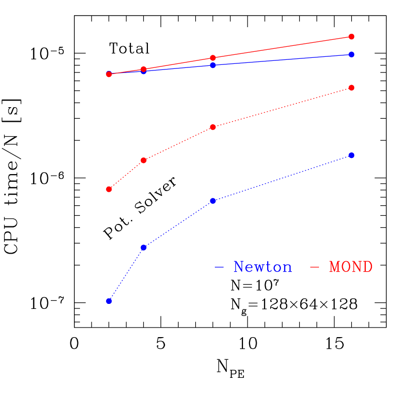
Figure 1: CPU time (summed over all PEs) per particle per timestep as a function of the number of PEs for N-MODY simulations of MOND (red) and Newtonian (blue) Hernquist (1990) spheres.

The computational time needed in the MOND potential solver scales roughly with the total number of grid points $N_{g}=(N_{r}+1)N_{\vartheta}N_{\varphi}$. In fact, in the serial version of the code (only one PE used), the MOND solver needs $\sim 10\%$ of the time spent to run particles, in a typical configuration where $N\sim 10N_{g}$. For large grids, and lower number of particles per cell, some advantages are obtained by parallelization of the MOND solver. To that purpose, when running with $N_{\rm PE}$ processors, N-MODY adopts a domain decomposition during the iteration cycle, by assigning at each PE only a sector of the $\vartheta$ coordinate containing $N_{\vartheta}/N_{\rm PE}$ grid points ($N_{\vartheta}\geq 4N_{\rm PE}$). This simple strategy results to be effective, even if several operations still require the full grid, resulting in $\sim 70\%$ of parallelization rate. In Fig. 1 we plot the CPU time (summed over all PEs) per timestep per particle as a function of the number of PEs for N-MODY simulations of a Hernquist (1990) sphere in Newtonian gravity (blue) and in MOND (red; with acceleration parameter $\kappa=1$, see Nipoti et al. 2007c). Both simulations, using $N=10^{7}$ particles and $N_{g}=128\times 64\times 128$ grid points, were run on an IBM Linux Cluster (Pentium IV/3 GHz PCs). In the diagram we distinguish the total CPU time (solid lines) and the CPU time spent by the potential solver (dotted lines). In all cases the total CPU time per particle is $\,\mathrel{\mathchoice{\lower 2.9pt\vbox{\halign{$\m@th\displaystyle\hfil#\hfil$\cr<\crcr\sim\crcr}}}{\lower 2.9pt\vbox{\halign{$\m@th\textstyle\hfil#\hfil$\cr<\crcr\sim\crcr}}}{\lower 2.9pt\vbox{\halign{$\m@th\scriptstyle\hfil#\hfil$\cr<\crcr\sim\crcr}}}{\lower 2.9pt\vbox{\halign{$\m@th\scriptscriptstyle\hfil#\hfil$\cr<\crcr\sim\crcr}}}\,}10^{-5}$ s, but it is apparent that the parallelization is not as efficient in MOND as in the case of Newtonian gravity. This is due to the contribution of the potential solver, which is only partially parallelized: while in Newtonian simulations the computational cost of the solver is always negligible, in MOND simulations it is non-negligible when $N_{\rm PE}\,\mathrel{\mathchoice{\lower 2.9pt\vbox{\halign{$\m@th\displaystyle\hfil#\hfil$\cr>\crcr\sim\crcr}}}{\lower 2.9pt\vbox{\halign{$\m@th\textstyle\hfil#\hfil$\cr>\crcr\sim\crcr}}}{\lower 2.9pt\vbox{\halign{$\m@th\scriptstyle\hfil#\hfil$\cr>\crcr\sim\crcr}}}{\lower 2.9pt\vbox{\halign{$\m@th\scriptscriptstyle\hfil#\hfil$\cr>\crcr\sim\crcr}}}\,}10$, because the iterative procedure requires a factor of 5-10 more time than the inversion of the Poisson equation.

We have already applied N-MODY to study dissipationless collapse (Nipoti et al. 2007a), phase mixing (Ciotti et al. 2007), galaxy merging (Nipoti et al. 2007c) and dynamical friction (Nipoti et al. 2008) in MOND. We found that these dynamical processes are profoundly different in MOND and in Newtonian gravity. In particular violent relaxation, phase mixing and merging take significantly longer in MOND than in Newtonian gravity, while dynamical friction is more effective in a MOND system than in an equivalent Newtonian system with dark matter.

N-MODY is publicly available upon request to the authors. It is written in FORTRAN 90 and can be compiled and run as either a parallel or a serial code.