Abstract

The well known (3+1) decomposition of Thorne and Macdonald is invoked to write down the Einstein-Maxwell equations generalised to (d+1) dimensions and also to formulate the plasma equations in a flat FRW like spacetime in higher dimensions (HD). Assuming an equation of state for the background metric we find solutions as also dispersion relations in different regimes of the universe in a unified manner both for magnetised(un) cold plasma. We find that for a free photon in expanding background we get maximum redshift in 4D spacetime, while for a particular dimension it is so in pre recombination era. Further wave propagation in magnetised plasma is possible for a restricted frequency range only, depending on the number of dimensions. Relevant to point out that unlike the special relativistic result this allowed range evolves with time. Interestingly the dielectric constant of the plasma media remains constant, not sharing the expansion of the background, which generalises a similar 4D result of Holcomb-Tajima in radiation background to the case of higher dimensions with cosmic matter obeying an equation of state . Further, analogous to the flat space static case we observe the phenomenon of Faraday rotation in higher dimensional case also.

KEYWORDS : cosmology; higher dimensions; plasma

PACS : 04.20, 04.50 +h

1. Introduction

While great strides have been made by general relativists to address the issues coming out of the recent observations in the field of astrophysics and cosmology and despite the fact that more than 90 percent of the cosmic stuff in stellar interior and intergalactic spaces is made up of matter in plasma state the much sought after union between the plasma dynamics and general relativity still remains elusive. Although we occasionally come across stray works like ‘plasma suppression of large scale structure formation in the universe’  [1] as also even the simulation techniques  [2] where it is argued that the geometry of the spacetime can be purported to be structured by observing sound waves in primordial plasmas the fact remains that as the field equations both in general relativity and plasma dynamics are highly nonlinear it is very difficult to obtain closed form solutions in physics. So either numerical relativity or a linearised approximation of the plasma equations is preferred, before going in for more complicated non linear phenomena. If we briefly trace the thermal history of the universe theorists believe that from approximately $t=10^{-3}$ s to $t=1$ s at temperatures $T>10^{10}$ K there was an electron positron plasma at ultra relativistic temperatures. With cooling the plasma comprises mainly electron and hydrogen ions, may be with small amount of helium and other light elements in thermal equilibrium with photons. This period has come to be known as radiation dominated era because it is believed that the energy density of photons much exceed that of matter  [3]. As the temperature decreased further with expansion at around $t\sim 10^{13}$ s recombination of ionized hydrogen atoms took place with consequent decoupling of matter and radiation and at a certain stage the universe becomes matter dominated. Consequently the temporal behaviour of the scale factor correspondingly changes with the evolution of matter at different time scales. Nevertheless, the studies of the effects of this expansion on the electromagnetic interactions of the matter, including the longitudinal and transverse modes have not, so far got the legitimate attention it deserves.

Another area of current interest is the role of an external magnetic field in many astrophysical systems and cosmology and possible sources for the field in different scales  [4] although the origin of the field continues to evade plausible physical explanations  [5] so far. Granted that temperature (particularly at early universe) is a known enemy of magnetism there are no compelling reasons why magnetic fields should not have been present in the early Universe either. Indeed, the presence of large scales magnetic fields in our observed Universe is a well established experimental fact. Since their first evidence in diffuse astrophysical plasmas beyond the solar corona  [4, 5] magnetic fields have been detected in our galaxy and in our local group through Zeeman splitting and through Faraday rotation measurements of linearly polarized radio waves. The Milky Way possesses a magnetic field whose strength is of the order of the microgauss corresponding to an energy density roughly comparable with the energy density today stored in the Cosmic Microwave Background Radiation (CMBR) energy spectrum peaked around a frequency of 30 GHz. Faraday rotation measurements of radio waves from extra-galactic sources also suggest that various spiral galaxies are endowed with magnetic fields whose intensities are of the same order as that of the Milky Way. The existence of magnetic fields at even larger scales (intergalactic scale, present horizon scale, etc.) cannot be excluded, but it is still quite debatable since, in principle, dispersion measurements (which estimate the electron density along the line of sight) cannot be applied in the intergalactic medium because of the absence of pulsar signals. Given the fact that a seed field does exist its amplification mechanism through the so called dynamo effect is relatively well understood  [6] for an expanding cosmological model with the help of magnetohydrodynamical (MHD) equations  [7]. On the other hand when discussing a primordial magnetic field one should also bear in mind that a large value would create significant anisotropy of the background geometry  [8] with consequent impact on CMBR findings. As the large scale isotropy of the CMBR fairly excludes that possibility there should be efficient mechanism to rapidly damp that field.

On the other hand there has been, of late, a resurgence of interests in physics in higher dimensional spacetime  [9] in its attempts to unify all the forces in nature, to give a physical explanation of the current accelerating era of the universe without bringing in any hypothetical quintessencial type of scalar field  [10] by hand, in the newly fashionable area of brane cosmology  [11] where the gravity is supposed to act in the bulk while other forces in the physical 3D space. It has also received serious attention in the recently proposed induced matter theory pioneered by Wesson and others [12]. Most importantly both higher dimensional spacetime and cosmological plasma have one thing in common - both are very relevant in the context of early universe. While early universe may be loosely viewed as the history of evolution of matter in plasma state it can also be shown that starting from a higher dimensional phase the Einstein’s generalized field equations dictate results such that as time evolves the 3D space expands while the extra dimensions shrink till plackian length when some stabilizing mechanism ( for example, quantum gravity, casimir effect, a repulsive potential) halts the shrinkage down to a very small length, say planckian size as to be invisible with the low energy physics at the moment. So the world around us appears manifestly three dimensional. But it should be emphasized that the time scales for the spontaneous self compactification (SSC) and the onset of nucleosynthesis clearly differ with SSC occurring much earlier. So many of our findings in MHD lose much of their relevance when working in higher dimensional spacetime. While literature abounds with works on the effects of the expanding background on the matter distribution and vice versa as also on a large number of other physical processes scant attention has been paid so far to address the issues resulting from the expanding universe on the propagation of say, electromagnetic wave as also its interactions in a plasma media. To authors’ knowledge Holcomb and Tajima (HT) [13, 14], Banerjee et al  [15] and later Dettmann et al  [16] made important contributions in this regard. HT investigated the electromagnetic wave propagation in a radiation dominated and later in a matter dominated background both with or without any plasma material and also generalised it to the magnetized case both warm and cold. For the ultra relativistic case it is observed that all the modes redshift at the same rate i.e., photons are, so to say, self similar. Though not explicitly pointed out in their works we think this, however, may be a direct consequence of the conformal flatness of the FRW metric chosen by them. Later Banerjee et al discussed this in a little more general way. Dettmann et al got the similar results starting from a kinetic theory approach. HT’s findings for the matter dominated model, however, differ sharply from the first paper in the sense that while in the unmagnetised plasma case the photons redshift identically but here for the Alfven waves the frequency redshifts in a bizarre fashion unlike the case of free photons, depending on the magnitudes of the plasma density and also strength of the external magnetic field. On the other hand Dettmann shows that even for the unmagnetised plasma the plasma oscillations and the photons do not share the identical temporal dependence if they are decoupled. They, however, treated the whole situation from kinetic energy considerations. In the present work we have investigated the plasma dynamics in an expanding higher dimensional background in a very general way. Taking a (d+1) dimensional flat FRW type of metric as background, which one of us  [17] derived earlier in a different context we first take the case of propagation of an electromagnetic wave in vacuum. To make things very general we assume an equation of state for the background as $p=\gamma\rho$. Taking $\gamma=\frac{1}{d}$, (as we are dealing with a (d+1) dimensional case) for the radiation and $\gamma=0$, for the dust case in the resulting solution we observe that solutions are very similar to the special relativistic form except that the frequencies red shift depending on $\gamma$ and the field amplitude is no longer a constant decaying with the expansion rate, reminiscent of the acoustic case where the damping occurs due to some form of dissipating mechanism. Here the expansion of the background, in a sense, takes the role of dissipation, causing this type of damping. It is observed that with number of dimensions the red shift decreases, being maximum in the usual 4D case. Moreover, red shift is less in the post recombination era compared to the early universe as expected. After briefly carrying out the so called $(3+1)$ decomposition of the Maxwell’s equations generalised to $(d+1)$ dimensional spacetime in section 2 we investigate the propagation of an electromagnetic wave in vacuum in section 3. In section 4 the electrostatic oscillations are very briefly discussed for a cold plasma and the dispersion relations obtained both for transverse and longitudinal modes. In section 5 we discuss in some detail the propagation of an electromagnetic wave in cold plasma in the presence of an ambient and homogeneous magnetic field both parallel and perpendicular to the wave propagator k. The presence of the magnetic field introduces newer and interesting modes of oscillation, creating Left and Right circularly polarized waves, resulting in the well known classical phenomenon of Faraday rotation. We also find that the wave propagation in the plasma is possible for certain range of frequencies only and this range critically depends on the number of dimensions. The paper ends with a short discussion in section 6.

2. Field Equations and its Formalism

We extend here the (3+1) decomposition of GR as formulated by Arnowitt, Deser and Misner (ADM)  [18] to a higher dimensional space time of (d+1) dimensions. The ADM formalism was developed mainly to address the issue associated with numerical relativity as also quantization of gravity fields, specially when the space time has considerable symmetry. This work is connected with plasma physics in curved space time. To make use of the intuition from the known results of MHD in flat spacetime it is preferable to spilt the ordinary electromagnetic field tensor $F^{\mu\nu}$ into electric and magnetic fields $E$ and $B$ in terms of which the field equations are more familiar. As the split formalism has been extensively discussed and used in the literature  [13, 14, 19] we shall very briefly touch upon its salient features as extended to higher dimensions.

We define a set of observers ( Fiducial Observers or FIDO ) at rest in the space spanned by the hypersurfaces of constant universal time, having a d-velocity vector field, $n$ orthogonal to spatial slices. It is well known that for a rotation-free space time ( as we are dealing here )

$$n_{i;j}=\sigma_{ij}+\frac{1}{d}~{}\theta\gamma_{ij}-a_{i}n_{j}$$ (1)

$(i,j=1,2,3,\ldots d)$ where $\sigma_{ij}$ is the shear of the Eulerian world lines given by

$$\sigma_{ij}\equiv\frac{1}{2}\left(n_{i;\mu}\gamma_{j}^{\mu}+n_{j;\mu}\gamma_{i}^{\mu}\right)-\frac{1}{d}~{}\theta\gamma_{ij}$$ (2)

Here $\gamma_{ij}$ is d-metric spatial tensors

$$a^{i}=n_{;j}^{i}n^{j}$$ (3)

and

$$\theta=n_{i}^{i}(=-K)$$ (4)

are the usual acceleration and expansion scalars and $K$ is the trace of the extrinsic curvature, $K_{;i}^{i}$.

For our metric we take the ( d+1) dimensional generalized FRW space time as

$$ds^{2}=dt^{2}-A^{2}\left(dx^{2}+dy^{2}+dz^{2}+d\psi_{n}^{2}\right)$$ (5)

(n = 5, 6, 7, …, d )

where $A\equiv A(t)$ is the scale function. For this particular metric two relevant quantities $\alpha=\frac{d\tau}{dt}$ ( the lapse function - the rate of change of fiducial proper time to that of universal time ) and also the shift vector $\beta$ ( signifying how much spatial co-ordinates are shifted as one moves from one hypersurface to the other ) naturally reduce to $\alpha=1$ and $\beta=0$.

In an earlier work  [17] one of us extensively discussed the ( d+1) dimensional isotropic and homogeneous space time and assuming an equation of state, $P=\gamma\rho$ found the scale factor as ( $P$ = pressure, $\rho$ = energy density )

$$A\sim t^{\frac{2}{d(1+\gamma)}}=t^{n},~{}~{}~{}n=\frac{2}{d(1+\gamma)}$$ (6)

With the extrinsic curvature scalar defined as

$$K=-\theta=-d\frac{\dot{A}}{A}=-d\frac{n}{t}$$ (7)

we finally write down the Maxwell’s equations  [20, 21, 22] (see Mcdonald et al for ( 3+1 ) split for more details ) generalized to ( d+1) dimensions as

$$\nabla.E = 4\pi\rho_{e}$$ (8)

$$\nabla.B = 0$$ (9)

$$\frac{\partial E}{\partial t} = KE+cA^{-1}\nabla\times B-4\pi J$$ (10)

$$\frac{\partial B}{\partial t} = KB-cA^{-1}\nabla\times E$$ (11)

$$\frac{\partial\rho_{e}}{\partial t} = K\rho_{e}-\nabla.J~{}\textrm{(charge ~{} conservation)}$$ (12)

and finally the particle equation of motion in $(d+1)$ dimensional as

$$\frac{DA^{d-1}p}{D\tau}=A^{d-1}q\left(E+A\frac{v}{c}\times B\right)$$ (13)

or

$$\frac{Dp}{D\tau}=\frac{d-1}{d}Kp+q\left(E+A\frac{v}{c}\times B\right)$$ (14)

where

$$\frac{D}{D\tau}=\frac{1}{\alpha}\left(\partial_{t}+v.\nabla\right)$$ (15)

is the convective derivative and the d- momentum

$$p=m_{e}\Gamma v$$ (16)

( $m_{e}$ is the rest mass, $\Gamma$ is the boost factor, and v, the d-velocity ). We thus see that for the simple metric given by equation(5)the decomposed ( d+1)- dimensional Maxwell equations closely mimic the flat space counterparts with some additional inputs from curved geometry( e.g., A and K terms).

Here $\nabla\cdot$ and $\nabla\times$ are the ordinary Minkowskian divergence and curl in Cartesian co-ordinates. In what follows we shall consider, for simplicity, the small amplitude linear theory such that the convective derivative simply reduces to ordinary derivative, $\frac{d}{dt}$.

3. Electromagnetic Waves in Vacuum

With the set of equations split to ( d + 1) formalism we are now in a position to attempt applications in varied plasma phenomena. To start with we discuss briefly the propagation of an electromagnetic wave in free space in the expanding back ground. Using equations (9-11) we get via $\nabla\cdot E=0$ (for vacuum) the wave equation as

$$A^{2}\ddot{E}+\left(2d+1\right)A\dot{A}\dot{E}+\left(d^{2}\dot{A}^{2}+dA\ddot{A}\right)E=c^{2}\nabla^{2}E$$ (17)

Assuming separation of variables in electric field

$$E(\textbf{x},t)=E_{t}E_{r}$$ (18)

we finally get

$$\ddot{E_{t}}+(2d+1)\frac{\dot{A}}{A}\dot{E_{t}}+\left[d\left(\frac{\ddot{A}}{A}+d\frac{\dot{A}^{2}}{A^{2}}\right)+\frac{k_{i}^{2}c^{2}}{A^{2}}\right]E_{t}=0$$ (19)

which, through equation (6) finally reduces to

$$t^{2}\ddot{E_{t}}+(2d+1)nt\dot{E_{t}}+\left[dn\left(dn+n-1\right)+k_{i}^{2}c^{2}t^{2(1-n)}\right]E_{t}=0$$ (20)

(here $k_{i}$ is a separation constant) corresponding to some initial fiducial time $t_{i}$. We shall subsequently see that $k_{i}$ is also identified with the $d$- dimensional wave vector.

On the other hand, as we are dealing with a homogeneous world the spatial equation remains unchanged yielding a solution $e^{i(k_{i}\cdot~{}r)}$ as in special theory of relativity. A little algebra shows that the time equation is reducible to a Bessel equation of order $\frac{1}{2}$ as in the 4D case. Thus dimensionality or the equation of state has apparently no role in determining the order of the equation. Plugging everything together we get

$$\textbf{E}=E_{0}\hat{e}t^{\frac{1-(2d+1)n}{2}}H_{\frac{1}{2}}^{(2)}\left[\frac{t^{1-n}}{1-n}k_{i}c\right]e^{ik_{i}.r}$$ (21)

where $H_{\frac{1}{2}}^{(2)}$ is a Hankel function of order $\frac{1}{2}$. Replacing the asymptotic form of $H_{\frac{1}{2}}$ we get

$$E=E_{0}i\sqrt{\frac{2k_{i}cd(1+\gamma)}{\pi\{d(1+\gamma)-2\}}}t^{-\frac{2}{1+\gamma}}e^{-\frac{ik_{i}cd(1+\gamma)}{d(1+\gamma)-2}t^{\frac{d(1+\gamma)-2}{d(1+\gamma)}}}e^{ik_{i}.r}$$ (22)

It represents a d-dimensional ‘damped’ harmonic wave as one encounters in mechanical vibration. While in mechanical motion the damping occurs due to friction here the expansion of the universe seemingly causes some sort of damping. For pre recombination era in $(d+1)$ dimensional space time $\gamma=\frac{1}{d}$ and the damping factor is $A^{-d}$. Hence the damping of the wave amplitude apparently decreases with number of dimensions. This finding merits some explanation. We have remarked earlier that the amplitude decay is somewhat geometrical in nature caused by the expansion and curvature. In that case as with dimension the expansion rate decreases one expects that damping should be larger in 4D but a little inspection of the last relation shows that when we plug in the expression of ‘$A$’ (equation (6)) the last relation further reduces to $t^{-\frac{2d}{d+1}}$. So the damping actually increases in higher dimensional spacetime. On the other hand, for a fixed $d$ the damping factor is $t^{-2}$ for post recombination era ($\gamma=0$) (see figure 1). Alternatively for the case of a very large number of dimensions the damping asymptotically reaches $t^{-2}$, a form set for post recombination era. It has not escaped our notice that the scaling of $E$ or $B$ for $\gamma=0$ is independent of the number of dimensions unlike the radiation case. So the amplitude factor gets increasingly damped as the universe ages. The fact that damping of the $E$ or $B$ increases with the number of dimensions in the early universe has a number of interesting theoretical implications. Firstly we mention in the introduction that in order that the universe evolves isotropically according to the FRW model there should be efficient mechanisms to damp the primordial magnetic field as early as possible. In that respect the HD spacetime has some inherent advantage over the standard 4D in the sense that the damping is faster in HD. Secondly the magnetic field at small scales may influence the bigbang nucleosynthesis and change the primordial abundances of light elements by significantly changing the expansion rate of the universe at the corresponding time. The success of the standard BBN scenario can provide an interesting set of bounds on the intensity of the magnetic field at that epoch  [5], indirectly constraining the number of dimensions of the spacetime. At this stage it may not be out of place to call attention to the fact that most of the above findings are of theoretical nature only and it is not feasible to relate them to current astrophysical data. Because multidimensional cosmological models lose much of their relevance well before the onset of bigbang nucleosynthesis and current observational findings can be explained for all practical purposes if the cosmological evolution be modelled along the standard four dimensional spacetime.

If as usual we set $k_{i}c=\omega_{i}$ ( the angular frequency of the wave at some initial time $t=t_{i}$ ) then the above equation may be rewritten as

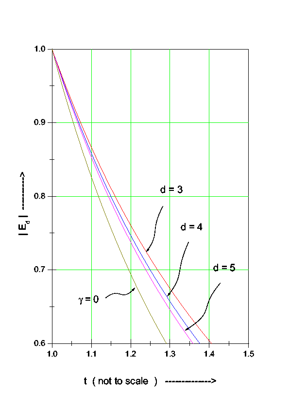
Figure 1: $\mid E_{d}\mid\sim t$ graph

$$E = E_{0}i\sqrt{\frac{2k_{i}cd(1+\gamma)}{\pi\{d(1+\gamma)-2\}}}t^{-\frac{2}{1+\gamma}}e^{-i\omega_{i}t\frac{d(1+\gamma)}{d(1+\gamma)-2}t^{-\frac{2}{d(1+\gamma)}}}e^{ik_{i}.r}$$ (23)

$$= E_{0}i\sqrt{\frac{2k_{i}cd(1+\gamma)}{\pi\{d(1+\gamma)-2\}}}t^{-\frac{2}{1+\gamma}}e^{-i\frac{d(1+\gamma)}{d(1+\gamma)-2}\omega_{d}t}e^{ik_{i}.r}$$

where

$$\omega_{d}=\omega_{i}t^{-\frac{2}{d(1+\gamma)}}$$ (24)

gives a measure of the red shift of the photon due to background expansion. For radiation dominated era $\gamma=\frac{1}{d}$ , $\omega_{d}=\omega_{i}t^{-\frac{2}{d+1}}$, so the rate at which the frequency decreases is maximum in 4D universe. Moreover damping is greater in radiation era (see figure 2).

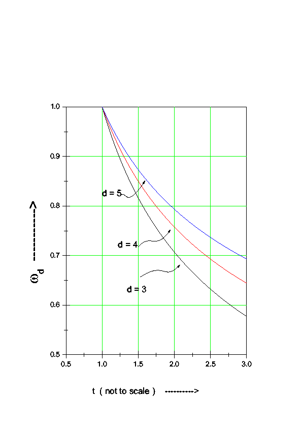
Figure 2: $\omega_{d}\sim t$ graph. As the number of dimension increases red shift decreases

Returning again to the equation (22) we see that the horizon for our metric is given by

$$L_{d}=\int\frac{cdt}{t^{\frac{2}{d(1+\gamma)}}}=\frac{d(1+\gamma)}{d(1+\gamma)-2}ct^{\frac{d(1+\gamma)-2}{d(1+\gamma)}}$$ (25)

so the equation may be recast as

$$E=E_{0}(x,t)e^{i({k.r-k_{i}.L_{d}})}=E_{0}(x,t)e^{ik_{i}(\hat{k}x-L)}$$ (26)

exactly similar to the Newtonian result where the horizon is simply $L=ct$.

4. Electrostatic Oscillation

In this section we shall very briefly consider an electromagnetic wave in a 2-component plasma. For simplicity we assume a small amplitude wave such that, $v\times B=0$ because it is of second order in perturbed quantities. This, in turn, allows us to neglect the motion of ions. Skipping intermediate mathematical steps for space we get via equations (14) and (16) for our metric (5)

$$v=\frac{iqt^{\frac{2}{d(1+\gamma)}}}{m_{e}\Gamma\omega_{i}}E=-\frac{ie}{m_{e}\Gamma\omega_{d}}E$$ (27)

The last equation is very similar to the flat space case except that here, $\omega_{d}$ is not a constant but shares the background expansion. When one uses the last equation in Maxwell equation (10) through $J=n_{0}qv$ we arrive at Coulomb’s law

$$\nabla\times B=-\frac{i\omega_{i}}{c}\epsilon E$$ (28)

where

$$\epsilon(\omega_{d})=1-\frac{\omega_{pT}^{2}}{\omega_{d}^{2}}$$ (29)

is the dielectric constant of the plasma medium with the suffix ${}^{\prime}T^{\prime}$ signifying transverse mode. The $\omega_{pT}^{2}$ is related to the well known plasma frequency  [23],

$$\omega_{p}^{2} = \frac{b_{d}n_{0}q^{2}}{m_{e}}~{},~{}~{}~{}\omega_{pT}^{2}\sim\frac{\omega_{p}^{2}}{\Gamma}$$

$$b_{d} = \frac{2^{\frac{d}{2}}\pi^{\frac{d}{2}}}{(d-1)!!}~{}~{}~{}~{}~{}~{}~{}~{}~{}~{}~{}~{}\mathrm{(d~{}~{}~{}even)},$$

$$= \frac{2^{(\frac{d+1)}{2}}\pi^{\frac{(d-1)}{2}}}{(d-2)!!}~{}~{}~{}~{}~{}~{}~{}~{}~{}\mathrm{(d~{}~{}odd)}$$

Skipping mathematical details it can also be shown that the transverse and the longitudinal modes give the dispersion relations as

$$\omega_{T}^{2}=\omega_{p}^{2}+c^{2}k^{2}$$ (30)

$$\omega_{L}^{2}=\omega_{p}^{2}$$ (31)

These relations are pretty well known in the special relativistic case, excepting that here all the quantities depend on time as well as the total number of dimensions.

Apparently the equation (29) has the same Newtonian form but both the frequencies depend on the scale factor, ‘$A$’ which, again, is a function of both the number of dimensions and the equation of state chosen.To end the section let us investigate the time dependence of the dielectric constant in equation(29). Now, $\omega_{pT}^{2}$ should share the time evolution of the background electron number density, $n_{0}$ ( the inverse of volume of the universe) i.e., $n_{0}\sim A^{-d}\sim t^{-\frac{2}{1+\gamma}}$. Again, from (27) we get, $v\Gamma\sim A^{n(1-d)}$. The equation (10) further dictates that $v\sim A^{-1}$, which gives $\Gamma\sim A^{(2-d)}$. So, $\omega_{pT}^{2}\sim\frac{n_{0}}{\Gamma}\sim A^{-2}\sim t^{-\frac{4}{d(1+\gamma)}}$. On the other hand the equation (24) implies that $\omega_{d}^{2}\sim A^{-2}$, hence $\epsilon$($\omega_{d}$) does not explicitly depend on time. This is a remarkable result in the sense that for a FRW type of metric the dielectric constant is a real constant irrespective of not only the total number of dimensions but also on the equation of state i.e., $\epsilon$($\omega_{d}$) continues to remain constant all through the evolution of the universe.

5. Electromagnetic Oscillations in Cold Plasma

In this section we investigate the situation where a plasma in thermodynamic equilibrium is slightly disturbed through the passage of an electromagnetic wave. We assume that an external ambient magnetic field is also present. We, however, assume the plasma medium to be cold so that the pressure can be neglected when considering the particle equation of motion. In stellar systems one often encounters situations where relaxation times are much larger than the age of the universe so that collisions ( hence pressure ) may be neglected. The effect of an electric field is not generally seriously considered because of the well known Debye shielding effect. The general problem of an electromagnetic wave propagating along an arbitrary direction with the external magnetic field is given by Appleton and Hartee in the Newtonian case when studying the propagation of radio waves in ionosphere. Holcomb  [14] studied in FRW metric a specialised situation of the A-H equation in the dust case. Considering the fact that a general solution with arbitrary $\theta$ is very difficult to tackle in an expanding background with arbitrary number of dimension we shall restrict ourselves to the cases when the electromagnetic wave propagates parallel and perpendicular to the magnetic field. However the topic is of great importance in astrophysics and space science where electromagnetic wave propagation in magnetized plasma is very relevant.

Case I ($\vec{B}\parallel\textbf{k}$) :

we assume that the external, uniform magnetic field and the wave vector $\mathbf{k}$ are both aligned along the $i^{th}$ direction (say z direction with $i=3$) in the $d$- dimensional space, such that $\textbf{k}=|k|\mathbf{e_{z}}$ and $\mathbf{B}=|B|\mathbf{e_{z}}$. As is customary in the analogous 3-dimensional static space we also assume that all the perturbed quantities have the same time dependence given by equation (23) such that the linearized equation of motion (13) takes the form

$$i\omega_{d}m_{e}v=e\left(E+A\frac{v}{c}\times B\right)$$ (32)

[ Here E is $\perp$r to $k$ and considering that we are dealing with a $(d+1)$ dimensional space time it has components $E_{1}$, $E_{2}$, $E_{3}$, $E_{4}$, …, $E_{j}$ . ]
Replacing $\frac{\partial E}{\partial t}$ via equation (23) by

$$\frac{\partial E}{\partial t}=-\left[i\omega_{d}+\frac{2}{(1+\gamma)t}\right]E$$ (33)

which, when plugged in equation (10) gives, after a long but fairly straight forward calculation gives for j=1

$$\left(\nabla\times B\right)_{1} = -\frac{i\omega_{d}}{c}A\left[\left(1-\frac{\omega_{p}^{2}}{\omega_{d}^{2}}\right)E_{1}-\frac{\omega_{p}^{2}}{\omega_{d}^{2}-\omega_{c}^{2}}\frac{\omega_{c}^{2}}{\omega_{d}^{2}}E_{1}+i\sum_{j=2}^{d}\frac{\omega_{p}^{2}}{\omega_{d}^{2}-\omega_{c}^{2}}\frac{\omega_{c}}{\omega_{d}}E_{j}\right]$$

$$=-i\frac{\omega_{d}}{c}\left[\left(1-\frac{\omega_{p}^{2}}{\omega_{d}^{2}-\omega_{c}^{2}}\right)E_{1}+i\sum_{j=2,j\neq 1}^{d}\frac{\omega_{c}}{\omega_{d}}\frac{\omega_{p}^{2}}{\omega_{d}^{2}-\omega_{c}^{2}}E_{j}\right]$$ (34)

For the case $j=3$ (i.e., along the direction of the magnetic field ) it takes a simple form

$$\left(\nabla\times B\right)_{3}=-i\frac{\omega_{d}}{c}\left(1-\frac{\omega_{p}^{2}}{\omega_{d}^{2}}\right)E_{3}$$ (35)

repeating the process for the remaining $(d-2)$ components we can write for the $\mu^{th}$ component a tensorial relation as

$$\left(\nabla\times B\right)_{\mu}=-i\frac{\omega_{d}}{c}\epsilon_{\mu\nu}E_{\nu}$$ (36)

($\mu,\nu=1,2,3,\ldots,d$). where $\epsilon_{\mu\nu}$ is rank 2 skew symmetric tensor of order ‘d’. A little inspection shows that

$$\epsilon_{11} = \epsilon_{22}=\epsilon_{44}=\epsilon_{55}=\ldots=\epsilon_{dd}=1-\frac{\omega_{p}^{2}}{\omega_{d}^{2}-\omega_{c}^{2}}=p_{1}\textrm{(say)}$$ (37)

$$\epsilon_{12} = \epsilon_{14}=\epsilon_{15}=\ldots=\epsilon_{1d}=\frac{\omega_{c}}{\omega_{d}}\frac{\omega_{p}^{2}}{\omega_{d}^{2}-\omega_{c}^{2}}=p_{2}$$ (38)

$$\epsilon_{31} = \epsilon_{32}=\epsilon_{34}=\ldots=\epsilon_{3d}=0$$ (39)

$$\epsilon_{33} = 1-\frac{\omega_{p}^{2}}{\omega_{d}^{2}}=p_{3}$$ (40)

so the $(d\times d)$ permitivity tensor comes out to be

$$\epsilon_{\mu\nu}=\left(\begin{array}[]{cccccc}p_{1}&ip_{2}&0&ip_{2}&.&ip_{d}\\ -ip_{2}&p_{1}&0&ip_{2}&.&0\\ 0&0&p_{3}&0&.&0\\ -ip_{2}&-ip_{2}&0&p_{1}&.&0\\ .&.&.&.&.&.\\ -ip_{d}&.&.&.&.&p_{1}\\ \end{array}\right)$$ (41)

Here $\omega_{p}$ is the plasma frequency given by

$$\omega_{p}^{2}=\frac{b_{d}n_{0}e^{2}}{m_{e}}$$ (42)

and the electron cyclotron frequency is given by

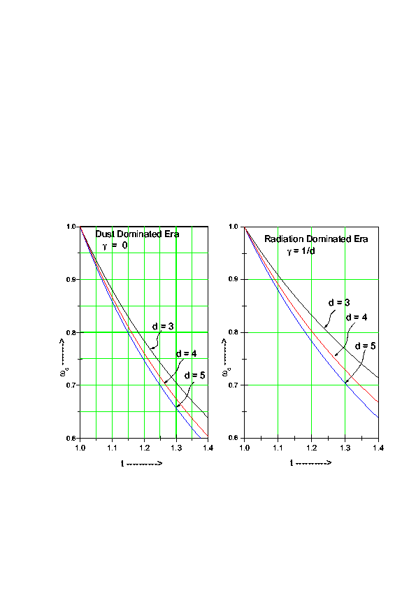
Figure 3: $\omega_{c}\sim t$ graph for both radiation and matter dominated era. As the number of dimension increases $\omega_{c}$ decreases. Further the decay is sharper in dust case compared to radiation case.

$$\omega_{c}=\frac{eB}{m_{e}c}t^{\frac{2}{d(1+\gamma)}}\equiv\frac{e\hat{B}}{m_{e}c}$$ (43)

where $\hat{B}$, the orthogonal magnitude of the ambient magnetic field is given by $\hat{B}=|(B)_{z}(B)^{z}|^{1/2}=Bt^{\frac{2}{d(1+\gamma)}}$ for our system (see figure 3).

If the magnetic field is switched off $(\omega_{c}=0)$ the equation (34) reduces to

$$\left(\nabla\times B\right)_{j}=-\frac{e\omega_{i}}{c}\epsilon E_{j}$$ (44)

exactly similar to the expression(28) of the section 4. Thus the introduction of the magnetic field generates varied modes transforming the dielectric constant scalar $\epsilon$ in equation (35) to a second rank tensor $\epsilon_{ij}$. Although the equations (30) - (40) exactly resemble the analogous expressions in Newtonian theory the fact remains that that all the frequencies now depend on time rather than being constant. Further the cyclotron frequency $\omega_{c}$ decays as $t^{-\frac{2(d-1)}{d(1+\gamma)}}$ exactly similar to the orthogonal component of the magnetic field.

If we take the curl of the equation (36) and replace $\nabla$ by $ik\hat{e_{z}}$, after a long but fairly straight forward calculation we are led to the matrix form

$$\left(\begin{array}[]{cccccc}(1-\frac{p_{1}}{\mathbf{n}^{2}})&-i\frac{p_{2}}{\mathbf{n}^{2}}&0&0&.&0\\ i\frac{p_{2}}{\mathbf{n}^{2}}&(1-\frac{p_{1}}{\mathbf{n}^{2}})&0&0&.&0\\ 0&0&-\frac{p_{3}}{\mathbf{n}^{2}}&0&.&0\\ .&.&.&.&.&.\\ .&.&.&.&.&.\\ 0&0&0&0&.&(1-\frac{p_{1}}{\mathbf{n}^{2}})\\ \end{array}\right)\left(\begin{array}[]{c}E_{1}\\ E_{2}\\ E_{3}\\ .\\ .\\ E_{d}\\ \end{array}\right)=\left(\begin{array}[]{c}0\\ 0\\ 0\\ .\\ .\\ 0\\ \end{array}\right)$$ (45)

where

$$\mathbf{n}^{2}=\frac{c^{2}k^{2}}{\omega_{i}^{2}}$$ (46)

where $\mathbf{n}$ is the refractive index of the plasma medium.

Three modes are possible.

First the longitudinal mode characterized by $E_{1}=E_{2}=E_{4}=\ldots=E_{d}=0$, ($E_{3}\neq 0$ and $p_{3}=0$). Since the displacement is along $Z$ direction the magnetic field has no role to play and $\omega_{d}=\omega_{p}$.

As we are more interested in the dynamics of the electromagnetic waves rather than the plasma oscillation as such we take $E_{3}=0$ in equation (45). Setting the determinant of the resulting $(d-1)\times(d-1)$ matrix in equation (45) to zero we get

$$\mathbf{n}^{2}=p_{1}\pm p_{2}$$ (47)

The plus sign gives via equation (36)

$$E_{\mu}-\emph{i}E_{\nu}=0~{}~{}~{}~{}~{}(\mathrm{\mu\neq\nu\neq 3}~{}~{}~{},~{}~{}~{}\emph{i}=\sqrt{-1})$$ (48)

such that

$$E_{l}=\left(\hat{e_{\mu}}-\emph{i}\hat{e_{\nu}}\right)e^{i(k_{L}z-\omega_{d}t)}$$ (49)

corresponding to left circularly polarized wave.

The wave number $k_{L}$ can be found from equations (37, 38, 46, 47) as

$$k_{L}=\frac{\omega_{d}}{c}\left[1-\frac{\omega_{p}^{2}}{\omega_{d}(\omega_{d}+\omega_{c})}\right]^{1/2}$$ (50)

On the other hand for the minus sign in (47) we get

$$E_{R}=\left(\hat{e_{\mu}}+\hat{e_{\nu}}\right)e^{[\emph{i}(k_{R}z-\omega t)]^{1/2}}$$ (51)

representing RCP wave with

$$k_{R}=\frac{\omega_{d}}{c}\left[1-\frac{\omega_{p}^{2}}{\omega_{d}(\omega_{d}-\omega_{c})}\right]^{1/2}$$ (52)

It is clear that the two eigen modes have different phase and group velocities and unlike the former case the Right Circularly Polarized (RCP) wave has a resonance at $\omega=\omega_{f}=\omega_{c}$ where the phase velocities vanish. The expressions so far exactly resemble the ones found in the propagation of an electromagnetic wave with an ambient magnetic field in Newtonian mechanics. However, here all the quantities $\omega_{d}$, $\omega_{p}$ etc. depend on time, a dependence modelled by the form of line-element, the number of dimensions and also the equation of state.

It should be noted that the time dependence of $\omega_{d}$ and $\omega_{c}$ are different being $\omega_{d}\sim t^{-\frac{2}{d(1+\gamma)}}$ and $\omega_{c}\sim t^{-\frac{2(d-1)}{d(1+\gamma)}}$. So there is no fixed resonant frequency as in Newtonian case but with time it changes.

It also follows from equation (52) that for

$$\omega_{d}=\omega_{1}=\frac{1}{2}\left[\omega_{c}+\sqrt{\omega_{c}^{2}+4\omega_{p}^{2}}\right]$$ (53)

the wave vector $k$ vanishes and our analysis breaks down. So the wave propagates for $\omega_{d}<\omega_{c}$ and $\omega_{1}<\omega_{d}$, otherwise it becomes evanescent. Moreover, as the temporal dependence of $\omega_{c}$ and $\omega_{d}$ are different the magnitude of the allowed region changes. With dimensions $\omega_{c}$ decays more sharply than $\omega_{d}$. Thus the propagation of the electromagnetic wave is more restricted in higher dimensions than the usual 4D.

Returning to the Left Circularly Polarized (LCP) wave we see that the wave vector vanishes for

$$\omega_{d}=\omega_{2}=\frac{1}{2}\left[-\omega_{c}+\sqrt{\omega_{c}^{2}+4\omega_{p}^{2}}\right]$$ (54)

and so the wave propagates for $\omega_{d}>\omega_{2}$

From what has been discussed above it is tempting to look for Faraday rotation (see ref. 4 for recent astrophysical data) analogous to the Newtonian case. Assuming that an electromagnetic wave traverses a distance $z$ in a plasma medium with a magnetic field subject to the restriction on frequencies discussed above the Faraday rotation is given by

$$\theta=\frac{k_{L}-k_{R}}{2}Z$$ (55)

It should be noted that one should revert to the physical co-ordinate rather than the co-moving one we are considering here. Accordingly $Z_{ph}=t^{-\frac{2}{d(1+\gamma)}}$, $Z_{cm}$ and $\theta$ finally comes out to be via equation (23)

$$\theta=\frac{k_{Li}-k_{Ri}}{2}Z_{ph}$$ (56)

with no dependence on time. so apparently the number of dimensions and the equation of state have no impact on this classical result. It may be relevant to mention that measurements of the radio waves from the extra galactic sources suggest that various spiral galaxies are endowed with magnetic fields whose intensities are of the same order of magnitude as that of Milky way  [4] i.e., of the order of microgauss corresponding to an energy density stored today in CMBR energy spectrum peaked around a frequency of 30 GHz.

Case II ($\vec{B}\bot\vec{k}$) :

Let us very briefly consider the case of a plasma with a uniform magnetic field $\textbf{B}=B_{0}\hat{e}_{z}$, through which an electromagnetic wave is propagating with propagation vector $\vec{\textbf{k}}=k\hat{e_{x}}$, perpendicular to the magnetic field. Here two modes are possible. As the mathematical exercise closely resembles the case I we shall totally skip intermediate steps to write the final form as

1. First mode (called ordinary wave) with displacements in z direction ( i.e. $\parallel B$) having the dispersion relation

$$\omega_{d}^{2}=\omega_{p}^{2}+k^{2}c^{2}$$ (57)

as the magnetic field has no influence for motion parallel to itself the equation (57) is exactly same as equation (30) for the electrostatic oscillation.

2. Second mode (called extraordinary wave) with displacements in (d-1)-dimensional hypersurface ($\bot B$) having dispersion relation

$$\frac{c^{2}k^{2}}{\omega_{d}^{2}}=1-\frac{\omega_{p}^{2}}{\omega_{d}^{2}}\frac{\omega_{d}^{2}-\omega_{p}^{2}}{\omega_{d}^{2}-\omega_{p}^{2}-\omega_{c}^{2}}$$ (58)

Before ending the section a final remark may be in order. We know that pulsars are rotating neutron stars giving out pulses of radio waves periodically, which are affected by the interstellar medium during their propagation to reach us. If the interstellar medium has a component of magnetic field parallel to propagation direction then as shown earlier the plane of polarization will suffer Faraday rotation depending on frequency, having a spread in the rotation angle. This spread may have, in principle at least, some imprint on the nature of expanding universe.

6. Discussion

With the help of (3+1) formalism the Einstein-Maxwell and the electrodynamical equations are written for a (d+1) dimensional FRW-like spacetime in presence of plasma and linearised equations are solved for different phases of the universe.The analysis essentially generalises to HD the well known results of Holcomb and Tajima. The salient features of our analysis may be summarised as:

1. For a propagating wave in HD in vacuum the photons redshift most in 4D and for a fixed $d$ in radiation dominated model.

2. Although the plasma is sharing the expansion of the background the dielectric constant remains a true constant. So the photons are in a sense self similar. This result was found earlier by Holcomb and Tajima. We here generalise this remarkable result to the case of extra dimensional spacetime and also for a fluid obeying a general equation of state. It may be tempting to suggest that the fact that the classical flat space result of the constancy of the dielectric constant is carried over to non static curved background and that too in higher dimensions may be due to the conformal flatness of the particular metric analysed here. So one should move with caution against any far fetched generalisation and in other complicated space time this result may not be true.

3. In the presence of an external magnetic field many interesting oscillation modes manifest themselves. A simplified Appleton-Hartee type of solution generalised to higher dimensions is obtained in curved spacetime. Only a selected range of frequencies are available for propagation here.

4. The well known phenomenon of Faraday rotation is obtained.

To end a final remark may be in order. The present work suffers from two serious disqualifications. For sake of mathematical simplicity we work out everything assuming a linearised plasma theory. Conditions under which one may assume linearized plasma theory may well exist in Newtonnian theory, but we are not being able to clearly formulate those things for the case of a nonflat spacetime and that too when it is expanding. Secondly most observational evidences suggest that even if one starts with a higher dimensional phase the universe underwent the self compactification transition much earlier than the epoch when the big bang nucleosynthesis sets in. So although literature abounds with works (for example, higher dimensional black holes and its thermodynamics etc.) studying the standard electromagnetic as well as MHD laws in the framework of multidimensions becomes a sort of suspect . In that sense our analysis is more of a purely theoretical nature without much direct physical applications. In future work one should try to generalise these results in the realm of non linear plasma and also attempt to relate some of our findings to known astrophysical data.

Acknowledgment : One of us(SC) acknowledges the financial support of UGC, New Delhi for carrying out this work.

References

- [1] Pisin Chen and Kwang- Chang Lai, 2007 Phys. Rev. Lett. 99 231302
- [2] G F Smoot, 2007 Rev. Mod. Phys. 79 1370
- [3] S Banerji and A Banerjee, 2007 General Relativity and Cosmology, Elsevier
- [4] P P Kronberg, 1994 Rep.Prog.Phy 57 325
- [5] M Gasperini, M Giovanini and G Veneziano,1995 Phy. Rev.Lett. 75 3796
- [6] R Beck, A Brandenberg, D Moss, A A Shukurov and D. Sokoloff,1996 Annu. Rev. Astron. Astrophys.34 155
- [7] C G Tsagas and J D Barrow , 1997 Class. Quant. Grav. 14 2539
- [8] Y B Zeldovich, A A Ruzmaikin and D D Sokoloff, 1983 Magnetic Fields in Astrophysics, ( Mcgraw Hill), N Y
- [9] D Hooper and S Profumo, ‘Dark Matter and Collider Phenomenology of Universal Extra Dimensions’, 2007 Physics Reports 453 p 27 - 115
- [10] S Chatterjee, A Banerjee and Z H Zhang, 2006 Int. J. Mod. Phys. A21 4035 ; N Banerjee and S Das, 2006 Mod. Phys. Lett. A 21 2663
- [11] U Debnath, A Banerjee and S Chakraborty , 2004 Class. Quant. Grav. 21 5609
- [12] P S Wesson, 1999 Space Time Matter ( World Scientific), Singapore
- [13] K A Holcomb and T Tajima, 1989 Phy. Rev. D40 3809
- [14] K A Holcomb, 1990 Astrophysical. J. 362 381
- [15] A Banerjee, S Chatterjee, A Sil and N Banerjee, 1994 Phy. Rev. D50 1161
- [16] C P Dettmann, N E Frankel, 1993 Phys. Rev. D48 5655
- [17] S Chatterjee and B Bhui, 1990 Mon. Not. R. Astron. Soc. 247 57
- [18] R Arnowitt, S Deser and C W Misner, in Gravitation: 1962 An Introduction to current Research, edited by L witten ( Wiley) New York
- [19] X H Zhang, 1989 Phy. Rev. D39 2933
- [20] D A Macdonald and K Thorne, 1982 Mon. Not. R. Astron. Soc. 198 345
- [21] K Thorne and D A Macdonald, 1982 Mon. Not. R. Astron. Soc. 198 339
- [22] C R Evans and J F Hawley, 1988 Astrophysical J. 332 659
- [23] V M Emelyanov, Yu P Nikitin, I L Rozenbal and A V Berkov , 1996 Phys.Rep. 143 p 1-68