Conjugate gradient heatbath for ill-conditioned actions

Abstract

We present a method for performing sampling from a Boltzmann distribution of an ill-conditioned quadratic action. This method is based on heatbath thermalization along a set of conjugate directions, generated via a conjugate-gradient procedure. The resulting scheme outperforms local updates for matrices with very high condition number, since it avoids the slowing down of modes with lower eigenvalue, and has some advantages over the global heatbath approach, compared to which it is more stable and allows for more freedom in devising case-specific optimizations.

A common problem in many branches of statistical physics is the sampling of distributions of the type $p\propto\exp\left(-\frac{1}{2}{\bf x\,\raisebox{0.0pt}[0.0pt][0.0pt]{\uuline{\mbox{$A$}}}\,x}\right)$ where  $\bf A$  is a positive definite $N\times N$ matrix and the random variable ${\bf x}$ an $N$-dimensional vector. Areas in which such sampling is needed are for instance QCDLüscher (1994); de Divitiis et al. (1995); de Forcrand (1999a) and a recently developed linear scaling electronic structure methodKrajewski and Parrinello (2005, 2006). In principle sampling $p$ is straightforward, if diagonalizing  $\bf A$  is an option. However, in many cases, $N$ is so large that circumventing the $\mathcal{O}\left(N^{3}\right)$ diagonalization step becomes mandatory. Different approaches have been proposed. In the so-called global heatbath method one writes $\,\raisebox{0.0pt}[0.0pt][0.0pt]{\uuline{\mbox{$\bf A$}}}\,=\,\raisebox{0.0pt}[0.0pt][0.0pt]{\uuline{\mbox{$\bf M$}}}\,^{T}\,\raisebox{0.0pt}[0.0pt][0.0pt]{\uuline{\mbox{$\bf M$}}}\,$, and obtains a series of statistically independent vectors by solving the linear system $\,\raisebox{0.0pt}[0.0pt][0.0pt]{\uuline{\mbox{$\bf M$}}}\,{\bf x}={\bf R}$, where ${\bf R}$ is a vector whose components are distributed according to a Gaussian with zero mean and unit variance $\left<R^{2}\right>=1$. The advantage of this method is that the algorithmic complexity of the problem can be reduced by using an iterative solver for the linear system. In order to expedite sampling a Metropolis-like criterion has been suggested that leads to correct sampling without having to bring the iterative process to full convergencede Forcrand (1999b); Wilcox (2002). Unfortunately, when the ratio between the largest and smallest eigenvalues is large (ill-conditioned matrices) the acceptance of this scheme drops to zero unless full convergency is achieved. An alternative approach is the local heatbath algorithm, in which at every step one single component of the state vector ${\bf x}$ is thermalized in turn, keeping the others fixed. It has been pointed out elsewhereGoodman and Sokal (1989); Adler (1989) that there is a close analogy between this second method and the Gauss-Seidel minimization technique. This approach is relatively inexpensive, but becomes very inefficient when the condition number of  $\bf A$  is large, and even more inefficient when the observable of interest depends strongly on the eigenvectors corresponding to smaller eigenvalues.

In this paper we propose a heatbath algorithm in which moves are performed along mutually conjugated directions. This choice is based on the analogy between various heatbath methods (see e.g. Ref. Goodman and Sokal (1989)) and directional minimization techniques. We show both analytically and numerically that the choice of conjugate directions allows all the degrees of freedom to become decorrelated on the same time scale, independent of their associated eigenvalue. We also discuss the cases in which the improved efficiency outbalances the additional computational cost. Our method can be interpreted as the subdivision of the global heatbath matrix inversion process into $N$ intermediate steps, all of which guarantee an exact sampling of the probability distribution.

In section I we introduce a simple formalism to treat heatbath moves along general directions, discuss the properties of a sweep through a set of conjugate directions, and describe a couple of algorithms to obtain such a set with reasonable effort. In section II we present some numerical tests on a model action and compare the efficiency of conjugate directions heatbath with local moves for a model observable. In section III we compare our method with global heatbath, and in section IV we present our conclusions.

I Collective modes heatbath

Given a probability distribution

$$P({\bf x})\propto\exp\left[-\left(\frac{1}{2}{\bf x}\,\raisebox{0.0pt}[0.0pt][0.0pt]{\uuline{\mbox{$\bf A$}}}\,{\bf x}-{\bf b}\cdot{\bf x}\right)\right]$$ (1)

a generic heatbath algorithm can be described as a stochastic process in which the vector ${\bf x}\left(t+1\right)$ is related to the vector at the previous step ${\bf x}\left(t\right)$ by

$${\bf x}\left(t+1\right)={\bf x}\left(t\right)+\tau{\bf d},$$ (2)

where ${\bf d}$ is a direction in the ${\bf x}$ space and

$$\tau=-\frac{{\bf d}\left(\,\raisebox{0.0pt}[0.0pt][0.0pt]{\uuline{\mbox{$\bf A$}}}\,{\bf x}-{\bf b}\right)}{{\bf d}\,\raisebox{0.0pt}[0.0pt][0.0pt]{\uuline{\mbox{$\bf A$}}}\,{\bf d}}+\left(\beta{\bf d}\,\raisebox{0.0pt}[0.0pt][0.0pt]{\uuline{\mbox{$\bf A$}}}\,{\bf d}\right)^{-1/2}R$$ (3)

where $R$ is a Gaussian random number with zero mean and unitary spread $\left<R^{2}\right>=1$, and $\beta$ is the inverse temperature at which the sampling is performed. The application of this algorithm does not require inversion of the matrix  $\bf A$ . The sequence of directions ${\bf d}$ is rather arbitrary, and could be a random sequence or a predefined deterministic sequence. Strictly speaking, detailed balance is satisfied only if the directions are randomly chosen at each step. Nevertheless it has been shown in RefManousiouthakis and Deem (1999) that correct sampling can be achieved if every Monte Carlo move leaves the equilibrium distribution unchanged. In Appendix A we show that this is the case, provided that direction ${\bf d}$ is chosen independently from position ${\bf x}$. Nevertheless, different choices of directions can lead to different sampling efficiency. Our final choice will be to select for ${\bf d}$ a sequence of conjugate directions (Section I.1). However, we shall first analyze the choice of random, uncorrelated directions, and a sequential sweep along a set of orthogonal directions.

For the sake of simplicity, we take ${\bf b}=0$ and we choose the basis into which  $\bf A$  is diagonal, $A_{ij}=a_{i}\delta_{ij}$. Since these properties are subsequently never used, no loss of generality is implied. To compare the efficiency of the different choices of directions we shall consider the autocorrelation matrix for the components along the eigenmodes $\left<x_{i}\left(0\right)x_{j}\left(t\right)\right>$. A quantitative measure of the speed of decorrelation of $\left<x_{i}\left(0\right)x_{j}\left(t\right)\right>$ can be obtained from its slope at the origin. Since in Monte Carlo one progresses in discrete steps, this quantity is given by

$$\left<x_{i}\left(0\right)x_{j}\left(1\right)\right>=\sqrt{\left<x_{i}\left(0\right)^{2}\right>\left<x_{j}\left(0\right)^{2}\right>}\left[\delta_{ij}-\Delta_{ij}\left({\bf d}\right)\right]$$ (4)

In Eq. (4) we have introduced the normalized slope tensor  $\boldsymbol{\Delta}$ , which can be expressed as a function of the eigenvalues of  $\bf A$  and of the components of ${\bf d}$, using equations (2) and (3):

$$\Delta_{ij}\left({\bf d}\right)=\frac{a_{i}h_{i}h_{j}}{\sum_{k}a_{k}h_{k}^{2}}\frac{\left<x_{i}\left(0\right)^{2}\right>}{\sqrt{\left<x_{i}\left(0\right)^{2}\right>\left<x_{j}\left(0\right)^{2}\right>}}=\frac{\sqrt{a_{i}a_{j}}d_{i}d_{j}}{\sum_{k}a_{k}d_{k}^{2}}$$ (5)

Therefore, depending on the choice of direction ${\bf d}$, the different components of the vector ${\bf x}$ decorrelate at different speeds. However, since $\operatorname{Tr}\,\raisebox{0.0pt}[0.0pt][0.0pt]{\uuline{\mbox{$\boldsymbol{\Delta}$}}}\,=1$, the sum of these normalized speeds does not depend on the direction chosen. The same quantity  $\boldsymbol{\Delta}$  also enters a recursion relation for the autocorrelation functions at a generic Monte Carlo step $t$,

$$\left<x_{i}\left(0\right)x_{j}\left(t+1\right)\right>=$$

$$\left<x_{i}\left(0\right)x_{j}\left(t\right)\right>-\sum_{k}\left[\left<x_{i}\left(0\right)x_{k}\left(t\right)\right>\sqrt{\frac{a_{k}}{a_{j}}}\Delta_{kj}\left({\bf d}\right)\right]$$ (6)

Use of this equation requires that one appropriately averages over the direction ${\bf d}$, as we shall discuss in the following.

We will begin our analysis from the simpler case, in which the direction ${\bf d}$ is chosen at every step to be equal to a stochastic vector ${\bf R}$, whose components are distributed as Gaussian random numbers with zero mean and standard deviation one. The normalized slope tensor (5) in this case results from an average over the possible directions,

$$\left<\Delta_{ij}\left({\bf d}={\bf R}\right)\right>=a_{i}\delta_{ij}\left<\frac{R_{i}^{2}}{\sum_{k}a_{k}R_{k}^{2}}\right>\overset{N\rightarrow\infty}{\approx}\frac{a_{i}\delta_{ij}}{\operatorname{Tr}\,\raisebox{0.0pt}[0.0pt][0.0pt]{\uuline{\mbox{$\bf A$}}}\,}.$$ (7)

The limit expression holds for the size $N$ of the matrix going to infinity (see Appendix B), under the hypothesis that the largest eigenvalue of  $\bf A$  does not grow with $N$ and that $\operatorname{Tr}\,\raisebox{0.0pt}[0.0pt][0.0pt]{\uuline{\mbox{$\bf A$}}}\,$ is $\mathcal{O}\left(N\right)$, hypotheses which are relevant to many physical problems. Since in this case the direction chosen at every step is independent of all the previous choices, the same average enters equation (6) at any time, so that proceeding by induction one can easily obtain the entire autocorrelation function,

$$\left<x_{i}\left(0\right)x_{j}\left(t\right)\right>=\delta_{ij}\left<x_{i}\left(0\right)^{2}\right>\left[1-\left<\Delta_{ij}\right>\right]^{t}$$ (8)

where $\left<\Delta_{ij}\right>$ is the quantity obtained in equation (7). From (8) we can calculate the autocorrelation time for mode $i$,

$$\tau_{i}=\frac{\sum_{t=0}^{\infty}\left<x_{i}\left(0\right)x_{i}\left(t\right)\right>}{\left<x_{i}^{2}\right>}=\left[a_{i}\left<\frac{R_{i}^{2}}{\sum_{k}a_{k}R_{k}^{2}}\right>\right]^{-1}\overset{N\rightarrow\infty}{\approx}\frac{\operatorname{Tr}\,\raisebox{0.0pt}[0.0pt][0.0pt]{\uuline{\mbox{$\bf A$}}}\,}{a_{i}}.$$

In the case of large $N$, the decorrelation speed of the components along normal modes is directly proportional to the corresponding eigenvalue, so that in ill-conditioned cases a critical slowing down for the softer normal modes will be present.

Let us now consider moves along a predefined set of orthogonal directions $\left\{{\bf u}^{(m)}\right\}_{m=0\ldots N-1}$. This is done to mimic the case in which one performs a sweep along Cartesian directions. In our reference frame, where  $\bf A$  is taken to be diagonal, this would be trivial, hence the choice of an arbitrarily oriented set of orthogonal directions. As in standard local heatbath, the outcome will depend on the orientation of the $\left\{{\bf u}^{(m)}\right\}$ relative to the eigenvectors of  $\bf A$ . Averaging over all the possible choices of initial direction, we find the slope at $t=0$,

$$\left<\Delta_{ij}\right>=\frac{1}{N}\sum_{m}\Delta_{ij}\left({\bf u}^{(m)}\right)=\frac{1}{N}\sum_{m}\frac{\sqrt{a_{i}a_{j}}u_{i}^{(m)}u_{j}^{(m)}}{\sum_{k}{a_{k}u_{k}^{(m)}}^{2}}$$ (9)

Obviously, it is not possible to reduce this result to an expression which does not depend on the particular set of orthogonal directions. However, the following inequality holds

$$\frac{a_{i}\delta_{ij}}{Na_{max}}\leq\left<\Delta_{ij}\right>\leq\frac{a_{i}\delta_{ij}}{Na_{min}}$$ (10)

Equation (10) does not put rigid constraints on the value of $\left<\Delta_{ij}\right>$, but demonstrates that also in this case  $\boldsymbol{\Delta}$  is diagonal and suggests that in real life the convergence will be faster for the higher eigenvalues, and that the spread in the relaxation speed for different modes is larger when the condition number $\kappa=a_{max}/a_{min}$ is higher.

In the case where directions $\left\{{\bf u}^{(m)}\right\}$ are swept sequentially we have not been able to derive a closed expression for $\left<x_{i}\left(0\right)x_{j}\left(t\right)\right>$ because of the dependence of ${\bf d}\left(t\right)$ on the previous history. If, on the other hand, a random direction is drawn from $\left\{{\bf u}^{(m)}\right\}$ at every step, $\left<x_{i}\left(0\right)x_{j}\left(t\right)\right>$ is given by expression (8) where $\left<\Delta_{ij}\right>$ has the value in equation (9).

I.1 Moves along conjugate directions

It is clear from equation (8) that a random choice of the directions ${\bf d}$ leads to fast decorrelation of the components relative to the eigenvectors with high eigenvalues. On the other hand, the components relative to the eigenvectors with low eigenvalues will decorrelate more slowly. Similar behavior is expected for the local heatbath method, unless particular relations hold between the eigenvectors and the Cartesian axes. If the operator  $\bf A$  is ill-conditioned, the practical consequence is that the slow modes will be accurately sampled only after a very large number of steps. As we have already discussed, the sum of the decorrelation slopes of the different components does not depend on the choice of the directions ${\bf d}$. However, with a proper choice of the directions ${\bf d}$ this sum could be spread in a uniform way among the different modes. A similar problem arises in minimization algorithms based on directional search, and is often solved choosing a sequence of conjugated directionsPress et al. (1986). In the same spirit, we can compute the decorrelation speed of the different modes when the ${\bf d}$’s are chosen to be conjugated directions. Let us consider a set of conjugated directions $\left\{{\bf h}^{(i)}\right\}$, such that ${\bf h}^{(i)}\,\raisebox{0.0pt}[0.0pt][0.0pt]{\uuline{\mbox{$\bf A$}}}\,{\bf h}^{(j)}=\delta_{ij}$. The set $\left\{{\bf h}^{(i)}\right\}$ can be generated with various algorithms, such as a Gram-Schmidt orthogonalization that uses the positive definite  $\bf A$  matrix as a metric, or a conjugate gradient procedure, as described in Section I.2.

Using the fact that $\sum_{k}h_{i}^{(k)}h_{j}^{(k)}=a_{i}^{-1}\delta_{ij}$, the slope at $t=0$ is

$$\left<\Delta_{ij}\right>=\frac{1}{N}\sum_{m}\frac{\sqrt{a_{i}a_{j}}h^{(m)}_{i}h^{(m)}_{j}}{{\bf h}^{(m)}\,\raisebox{0.0pt}[0.0pt][0.0pt]{\uuline{\mbox{$\bf A$}}}\,{\bf h}^{(m)}}=$$

$$=\frac{1}{N}\sqrt{\frac{a_{j}}{a_{i}}}\sum_{m}\frac{a_{i}h^{(m)}_{i}h^{(m)}_{j}}{{\bf h}^{(m)}\,\raisebox{0.0pt}[0.0pt][0.0pt]{\uuline{\mbox{$\bf A$}}}\,{\bf h}^{(m)}}=\frac{\delta_{ij}}{N}$$

With this choice, the decorrelation slopes of the different modes are independent of the eigenvalue. If one chooses one conjugate direction at random at each step it is straightforward to show that overall the autocorrelation function decays exponentially as

$$\left<x_{i}\left(0\right)x_{j}\left(t\right)\right>=\delta_{ij}\left<x_{i}\left(0\right)^{2}\right>\left[1-\frac{1}{N}\right]^{t}$$

This derivation shows that if matrix  $\bf A$  is ill-conditioned and one wishes to decorrelate the slow modes, then the choice of performing the heatbath using a sequence of conjugated directions can improve the sampling quality dramatically. Of course, the slow modes are accelerated and the fast modes are decelerated. However, it is clear that a completely independent vector ${\bf x}$ is obtained only when all the modes are decorrelated. A heatbath on conjugate directions allows all the modes to be decorrelated with the same efficiency, irrespective of their stiffness. Even better efficiency can be obtained by sequentially sweeping a set of conjugated directions. At first sight it would appear that the dependence of ${\bf h}\left(t\right)$ on ${\bf h}\left(t-1\right)$ would make it very difficult if not impossible to obtain the autocorrelation function in a closed form. However, conjugate directions have a redeeming feature. If we expand the position vector on the non-orthogonal basis $\left\{{\bf h}^{(m)}\right\}$, ${\bf x}=\sum_{i}\alpha^{i}{\bf h}^{(i)}$, and we evaluate the correlation matrix between the contravariant components $\alpha^{i}$, we find that $\left<\alpha^{i}\alpha^{j}\right>=\delta_{ij}$. This property can be easily demonstrated taking into account that the ensemble average $\left<x_{i}x_{j}\right>=A^{-1}_{ij}$, and that conjugacy implies ${\bf h}^{(i)}\,\raisebox{0.0pt}[0.0pt][0.0pt]{\uuline{\mbox{$\bf A$}}}\,{\bf h}^{(j)}=\delta_{ij}$. Thus, effectively, every time we perform a heatbath move along direction ${\bf h}^{(i)}$ the component $\alpha^{i}$ is randomized, without affecting the others. After a complete sweep across the set of directions a completely independent state is obtained.

A more formal proof is provided in appendix C, where it is also demonstrated that the autocorrelation function is

$$\left<x_{i}\left(0\right)x_{i}\left(t\right)\right>=\left<x_{i}\left(0\right)^{2}\right>\left\{\begin{array}[]{cc}\left[1-\frac{t}{N}\right]&t<N\\ 0&t\geq N\end{array}\right.$$ (11)

Therefore the corresponding autocorrelation time is $\tau_{i}=\left(N+1\right)/2$. A remarkable feature of equation (11) is that the autocorrelation function is linear, and that after $N$ moves a completely independent vector is obtained. This property holds also for the global heatbath method. In Section III we shall discuss the relation between our approach and global heatbath sampling.

I.2 Conjugate-gradient approach to generate conjugate directions

In the last section we have shown how a heatbath algorithm based on conjugate directions can dramatically improve the sampling of the slow modes for an ill-conditioned action. An efficient strategy to generate these directions is the application of the conjugate gradient procedurePress et al. (1986). For the sake of completeness and to introduce a consistent notation we give here an outline of the CG algorithm. One starts from a random configuration and search direction, ${\bf h}^{(0)}={\bf g}^{(0)}={\bf R}$, so that the directions obtained and the sample vector ${\bf x}$ are independent as required. Then, a series of directions ${\bf h}^{(m)}$ and residuals ${\bf g}^{(m)}$ are generated using the recurrence relations

$${\bf g}^{(i+1)}={\bf g}^{(i)}-\lambda_{i}\,\raisebox{0.0pt}[0.0pt][0.0pt]{\uuline{\mbox{$\bf A$}}}\,\cdot{\bf h}^{(i)}\quad{\bf h}^{(i+1)}={\bf g}^{(i+1)}+\gamma_{i}\cdot{\bf h}^{(i)}$$

$$\lambda_{i}=\frac{{\bf g}^{(i)}\cdot{\bf g}^{(i)}}{{\bf h}^{(i)}\,\raisebox{0.0pt}[0.0pt][0.0pt]{\uuline{\mbox{$\bf A$}}}\,{\bf h}^{(i)}}\quad\gamma_{i}=\frac{{\bf g}^{(i+1)}\cdot{\bf g}^{(i+1)}}{{\bf g}^{(i)}\cdot{\bf g}^{(i)}}$$

This procedure generates at every step a new direction ${\bf h}^{(i)}$, conjugated to all the previous ones, and it can be used to perform a directional heatbath move on ${\bf x}$. It should be stressed that there is no need to store all the ${\bf h}^{(i)}$ if the heatbath moves are performed concurrently with the CG minimization. The “force” $\,\raisebox{0.0pt}[0.0pt][0.0pt]{\uuline{\mbox{$\bf A$}}}\,{\bf h}^{(i)}$ can be reused for performing the heatbath update (cfr. Eq. (2)). At a certain point the CG procedure will be over, with the residual ${\bf g}$ dropping to zero. The sequential sweep algorithm described inte the previous section can be implemented starting again from the same ${\bf g}^{(0)}$.

In contrast to the global heatbath method, numerical stability is not a major issue, since the accuracy of the sampling does not depend on the search directions being exactly conjugated. The only effect of imperfect conjugation would be to slightly reduce the decorrelation efficiency. There is however a drawback to this approach. In order to be ergodic, the set of directions must span the whole space. The problem arises when there are degenerate eigenvalues, as CG converges to zero in a number $p$ of iterations equal to the number of distinct eigenvalues. If we keep reusing the same set of $p<N$ directions, only a part of the subspaces corresponding to degenerate eigenvalues will be explored, and the sampling will not be ergodic.

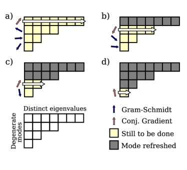
Figure 1: Scheme of the block algorithm described in paragraph I.2; squares represent eigenvectors of the action matrix, which need to be refreshed in order to obtain a statistically independent sample point; modes on the same column correspond to the same, degenerate eigenvalue. At every step, one of the vectors of a set with the same size as the biggest degenerate subspace is used in a conjugate gradient minimization, while the remaining ones are made orthogonal to the search directions that are generated in the process. When the first vector approaches zero, one can start back on the second one (Figure b)), and the process can be continued (Figures c) and d)) until the refresh is complete.

We have considered two possible ways of recovering ergodicity. The simplest consists in drawing a new random point ${\bf g}^{(0)}={\bf R}$ every time we reset the CG search. This causes a deviation from the linear behavior of the autocorrelation functions for $t\approx N$. Non-degenerate eigenvalues will initially converge with $-1/p$ instead of $-1/N$ slope, but degenerate ones will converge more slowly, and with exponential trend, as we are sampling random directions within every degenerate subspace.

In order to improve the efficiency, we mix CG with Gram-Schmidt orthogonalization of a small set of vectors, ideally of the same size $d$ of the largest degeneracy present. As discussed earlier, here Gram-Schmidt orthogonalization has to be performed using the metric of  $\bf A$ , which amounts to imposing conjugacy. The procedure is illustrated in Figure 1. We start from $d$ random vectors, $\left\{{\bf v}^{(j)}\right\}_{j=0..d-1}$. We set ${\bf h}^{(0)}={\bf g}^{(0)}={\bf v}^{(0)}$ and begin a CG minimization. At each step we obtain a search direction ${\bf h}^{(i)}$, and make each of the other $d-1$ vectors conjugate to ${\bf h}^{(i)}$ with a Gram-Schmidt procedure. This does not require any matrix-vector product other than the one necessary for the heatbath step. After $p$ iterations the conjugate gradient will have converged and ${\bf g}$ will be close to zero. We can start again from the second vector in the pool, which meanwhile has become $\bar{\bf v}^{(1)}$, and is conjugate to all the directions visited so far. Thus, we set ${\bf h}^{(0)}={\bf g}^{(0)}=\bar{\bf v}^{(1)}$ and start again the CG procedure, orthogonalizing the $d-2$ remaining vectors to ${\bf h}^{(i)}$, and so on and so forth. After $N$ steps the procedure will be converged. At the successive sweep, one can generate again a set of random initial $\left\{{\bf v}^{(j)}\right\}$. This can make the method more stable, at the cost of some loss in performance. Some savings can be made if one stores the conjugated $\bar{\bf v}^{(i)}$, and uses them in the subsequent sweeps, avoiding the need to repeat the GS orthogonalizations (see figure 1). In practice, where more than one complete sweep is affordable, it is easy to devise adaptive variations of this scheme, in which the pool of vectors $\left\{{\bf v}^{(j)}\right\}$ is enlarged whenever the CG minimization converges in less than $N$ steps, so that in a few sweeps the optimal size to guarantee ergodicity is attained.

II Benchmarks and comparison with local heatbath

In the previous section we have discussed a collective modes heatbath method that could outperform standard local heatbath techniques when the Hamiltonian has a very large condition number and sampling along the slower eigenmodes is required. In this section we illustrate the efficiency of our algorithm using numerical experiments on a simple model for  $\bf A$ ,

$$\,\raisebox{0.0pt}[0.0pt][0.0pt]{\uuline{\mbox{$\bf A$}}}\,=\,\raisebox{0.0pt}[0.0pt][0.0pt]{\uuline{\mbox{$\bf 1$}}}\,+\left(\begin{array}[]{cccccc}-2b&b&0&\cdots&0&b\\ b&-2b&b&0&\cdots&0\\ 0&b&-2b&b&\ddots&\vdots\\ \vdots&0&b&-2b&\ddots&0\\ 0&\vdots&\ddots&\ddots&\ddots&b\\ b&0&\cdots&0&b&-2b\end{array}\right)$$ (12)

This matrix corresponds to the dynamical matrix of a linear chain of spring-connected masses, with periodic boundary conditions and an additional diagonal term to make the acoustic mode nonzero. $b$ can be chosen so as to obtain the desired condition number. Eigenmodes and eigenvalues for such a matrix are easily obtained,

$$a_{k}=1+2b\left(1-\cos\frac{2k\pi}{N}\right)$$

$$u^{(k)}_{l}=\sqrt{\frac{1+\delta_{0k}+\delta_{N/2,k}}{N}}\left\{\begin{array}[]{lc}\cos\frac{2kl\pi}{N}&k\leq N/2\\ \sin\frac{2kl\pi}{N}&k>N/2\end{array}\right.$$

and projection of a state on the eigenvectors is quickly done via fast-Fourier transform. In Figure 2 we compare the the autocorrelation functions obtained with different algorithms for a matrix of the form (12). Figure 2 also highlights the ergodicity problems connected with the naive use of the conjugate gradient algorithm to generate the search directions, and shows how both the suggestions of paragraph I.2 can help in solving this problem. In general, a conjugate directions search speeds up decorrelation for the slower modes, but is less efficient than local heatbath for the modes with a high eigenvalue. This is a direct consequence of the fact that $\operatorname{Tr}\,\raisebox{0.0pt}[0.0pt][0.0pt]{\uuline{\mbox{$\boldsymbol{\Delta}$}}}\,=1$. An additional advantage of our method is the linear rate of decorrelation, which allows complete decorrelation just like the direct inversion of  $\bf M$ , whereas moves along the Cartesian axes lead to approximatively exponential autocorrelation functions.

Figure 2: Autocorrelation functions for a) the projection along the mode $a_{0}=1$; b) the projection along the mode $a_{4}\approx 9.8$ for a matrix of the form (12) with $N=100$ and condition number $\kappa=10^{3}$. Line A corresponds to local heatbath moves (one step stands for a complete sweep of the $N$ coordinates), lines B to D to conjugate directions moves: B is the hybrid conjugate gradient/Gram-Schmidt block algorithm; C corresponds to CG sweeps, with the search direction randomized at the beginning of every sweep; curve D corresponds to CG sweeps starting from the same initial vector. Conjugate direction moves decorrelate faster than local heatbath for the slow mode, but are less efficient for modes with higher eigenvalue. For degenerate eigenmodes, the method used for curve D is not ergodic (and thus gives incorrect values for $\left<x_{i}^{2}\right>$), and random restarts (curve C) are much less efficient than the hybrid (curve B) algorithm.

We stress again that the relative efficiency of the two methods depends strongly on the observable being calculated and on the actual spectrum of the Hamiltonian of the system. As a more realistic benchmark we will consider the evaluation of the trace of the inverse matrix, i.e.

$$\Omega=\operatorname{Tr}\left(\,\raisebox{0.0pt}[0.0pt][0.0pt]{\uuline{\mbox{$\bf A$}}}\,^{-1}\right)=\left<{\bf x}^{2}\right>$$ (13)

This observable is strongly dependent on the slow modes.

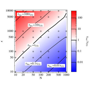
Figure 3: (Color online) Comparison of the efficiency of local heatbath versus conjugate-gradient moves. The graph represents $\tau_{CG}/\tau_{loc}$, the ratio of the autocorrelation times for the observable $\Omega$ (13); $\tau_{loc}$ corresponds to the value obtained from standard local heatbath moves (one unit of Monte Carlo time corresponds to a whole coordinates sweep), while $\tau_{CG}$ corresponds to the value obtained with moves along conjugate directions, as obtained from our block algorithm with random restarts. The data plotted results from a linear interpolation of some simulations (labeled by $\otimes$) performed for an action of the form (12), with varying size $N$ and condition number $\kappa$.

In Figure 3 we plot the ratios of the autocorrelation times $\tau\left[\Omega\right]$ as obtained with local heatbath moves and with the block conjugate gradient version of our algorithm, as a function of changing condition number and system size.

III Comparison with global heatbath

It remains for us to discuss how our method fares in comparison with global heatbath. The latter requires that matrix  $\bf A$  be decomposable in the form $\,\raisebox{0.0pt}[0.0pt][0.0pt]{\uuline{\mbox{$\bf A$}}}\,=\,\raisebox{0.0pt}[0.0pt][0.0pt]{\uuline{\mbox{$\bf M$}}}\,^{T}\,\raisebox{0.0pt}[0.0pt][0.0pt]{\uuline{\mbox{$\bf M$}}}\,$. This is the case in many fieldsKrajewski and Parrinello (2005), but in principle if it were necessary to decompose  $\bf A$  this would add extra cost. Here we make our comparison assuming that  $\bf M$  is already available. In such a case, the two algorithms are on paper equally efficient in producing statistically independent samples. The global heatbath might offer some numerical advantages when the spectrum of  $\bf M$  is highly degenerate, since the number of CG iterations needed to solve the $\,\raisebox{0.0pt}[0.0pt][0.0pt]{\uuline{\mbox{$\bf M$}}}\,x={\bf R}$ linear system is $p<N$, as discussed earlier. Whenever a good preconditioner for the linear system is available, other inversion algorithms such as the stabilized bi-conjugate gradientVan Der Vorst (1992) or the generalized conjugate residual may allow to solve the linear system with a sufficient accuracy more efficiently than using CG. In this paper we make the comparison with conjugate gradient because of the close analogy with our scheme and because our method is aimed at problems where ill-conditioning cannot be otherwise relieved.

In this respect, our method displays significant advantages. Firstly, it is more stable, because every move preserves the probability distribution, and the conjugate gradient procedure (which is known to be quite delicate in problems with large condition number) is only used to generate search directions. Instabilities in the procedure, which would cause incorrect sampling in the global heatbath, affect only the efficiency, and not the accuracy. Moreover, dividing the $N$ steps of an iterative inversion process into separate heatbath moves greatly improves the flexibility of the sampling scheme. To give some examples, if one needs to perform an average on a slowly varying  $\bf A$ , it is possible to perform only a partial sweep with fixed action, then continue with the new  $\bf A$ , assuming that eigenmodes will change slowly. It is also straightforward to tailor the choice of directions in order to optimize the convergence speed for the observable or interest. Adler’s overrelaxationAdler (1981) can be included naturally, and can help in further optimizing the autocorrelation time. As an example of possible fine-tunings, let us recall the observable $\Omega$ introduced in the previous section (equation (13)). This observable depends strongly on the softer eigenvector of  $\bf{A}$ . We have then modified our algorithm in the following way: we perform block conjugate gradient sweeps, with random resets, and we monitor the curvature along the direction being thermalized, ${\bf h}\,\raisebox{0.0pt}[0.0pt][0.0pt]{\uuline{\mbox{$\bf A$}}}\,{\bf h}/{\bf h}\cdot{\bf h}$. We save the direction of minimum curvature encountered along the sweep, ${\bf h}_{min}$; during the following sweep, every $m$ moves along the CG directions, one move is performed along ${\bf h}_{min}$. As is evident from Figure 4, this trick considerably reduces the autocorrelation time for $\Omega$. Even smarter combinations of moves can be devised, and the one we suggest is just an example of how the additional flexibility gained through subdividing the inversion process in $N$ exact sampling moves can be exploited. In Table 1 we report some numerical extimates of the error in the evaluation or $\Omega$, which can serve as a reference to compare our method to other approaches.

Table 1: Percentual errors in the evaluation of $\Omega=\left<{\bf x^{2}}\right>$ (equation (13)), extimated using a blocking analysis, for different sampling methods. A corresponds to local heatbath, B corresponds to “hybrid” versions of our CG algorithm, with a pool of two vectors with random restarts, while curve C is obtained including the tricks described in section III with $m=50$. Different tests are performed with varying matrix size $N$, number of sampling steps $T$ and condition number $\kappa$. Due to the large autocorrelation time, the values of the error for local heatbath with $N=100$ and $T=10^{6}$ could not be extimated as reliably as in the other cases, and are only indicative.

$N$	$\kappa$	$T$	A	B	C
$10^{3}$	$5\times 10^{4}$	$10^{6}$	4.0	1.5	1.4
$10^{3}$	$5\times 10^{4}$	$10^{7}$	1.3	0.51	0.45
$10^{3}$	$5\times 10^{3}$	$10^{6}$	0.78	0.85	0.85
$10^{3}$	$5\times 10^{3}$	$10^{7}$	0.24	0.28	0.28
$100$	$5\times 10^{4}$	$10^{6}$	$\sim$11	1.2	1.1
$100$	$5\times 10^{4}$	$10^{7}$	4.9	0.44	0.34
$100$	$5\times 10^{3}$	$10^{6}$	$\sim$3	0.88	0.82
$100$	$5\times 10^{3}$	$10^{7}$	1.1	0.30	0.25

Figure 4: Autocorrelation function for the observable (13) for an action of the form (12), with size $N=100$ and condition number $\kappa=5\times 10^{3}$. Line A corresponds to local heatbath, line B to the “hybrid” versions of our CG algorithm, with a pool of two vectors with random restarts, while curve C is obtained including the tricks described in section III with $m=5$

IV Conclusions

We have presented an algorithm for performing collective modes heatbath along conjugate directions for a quadratic action, which allows the components of the sampling vector along all modes to be decorrelated in $N$ steps, with a linear decay to zero. This method is more computationally demanding than local updates, but becomes competitive for ill-conditioned actions, when one needs to compute observables which depend on modes with low eigenvalues, or when the spectrum of the action matrix has only a few high eigenvalue modes which would slow down Cartesian moves. In fact, this method has an efficiency comparable with that of direct inversion of the matrix, but presents various advantages, such as improved stability, as the numerical issues connected with conjugate gradient method do not affect the accuracy of the sampling, and the possibility of exploiting some additional flexibility to improve the sampling on a case-by-case basis. Lastly, global heatbath requires the knowledge of the square root of the action  $\bf A$ , so our scheme should be considered whenever the square root is difficult to compute or its use is inefficient with respect to the original action.

The geometrical simplicity of this approach, with its close analogy with minimization methods, also suggests that it might be extended to the sampling of anharmonic systems.

Appendix A

We report here a simple demonstration of the fact that heatbath moves along a generic direction ${\bf d}$ leave an equilibrium probability distribution unchanged. We will use the fact that if ${\bf R}$, ${\bf R}^{\prime}$ and ${\bf R}^{\prime\prime}$ are vectors distributed as Gaussians with zero mean and standard deviation one, then $\,\raisebox{0.0pt}[0.0pt][0.0pt]{\uuline{\mbox{$\bf B$}}}\,{\bf R}+\,\raisebox{0.0pt}[0.0pt][0.0pt]{\uuline{\mbox{$\bf C$}}}\,{\bf R}^{\prime}$ is distributed as $\,\raisebox{0.0pt}[0.0pt][0.0pt]{\uuline{\mbox{$\bf D$}}}\,{\bf R}^{\prime\prime}$ where $\,\raisebox{0.0pt}[0.0pt][0.0pt]{\uuline{\mbox{$\bf D$}}}\,^{T}\,\raisebox{0.0pt}[0.0pt][0.0pt]{\uuline{\mbox{$\bf D$}}}\,=\,\raisebox{0.0pt}[0.0pt][0.0pt]{\uuline{\mbox{$\bf B$}}}\,^{T}\,\raisebox{0.0pt}[0.0pt][0.0pt]{\uuline{\mbox{$\bf B$}}}\,+\,\raisebox{0.0pt}[0.0pt][0.0pt]{\uuline{\mbox{$\bf C$}}}\,^{T}\,\raisebox{0.0pt}[0.0pt][0.0pt]{\uuline{\mbox{$\bf C$}}}\,$. Since ${\bf x}$ is drawn from the equilibrium distribution, i.e. ${\bf x}=\,\raisebox{0.0pt}[0.0pt][0.0pt]{\uuline{\mbox{$\bf M$}}}\,^{-1}{\bf R}$, we can cast Eq. (3) and (2) into the form

$$x_{j}^{\prime}=\sum_{m}P_{jm}R_{m}+\sum_{m}Q_{jm}R_{m}^{\prime}$$

$$P_{jm}=\left(\,\raisebox{0.0pt}[0.0pt][0.0pt]{\uuline{\mbox{$\bf M$}}}\,^{-1}\right)_{jm}-d_{j}\sum_{k}M_{km}d_{k}\quad\quad Q_{jm}=d_{j}\delta_{m0}$$

where we have put ${\bf b}=0$ into Eq. (3) and normalized the direction so that ${\bf d}\,\raisebox{0.0pt}[0.0pt][0.0pt]{\uuline{\mbox{$\bf A$}}}\,{\bf d}=1$ in order to simplify the notation. We can then compute

$$\sum_{m}P_{jm}P_{lm}=\,\raisebox{0.0pt}[0.0pt][0.0pt]{\uuline{\mbox{$\bf A$}}}\,^{-1}_{jl}-d_{j}d_{l}\quad\quad\sum_{m}Q_{jm}Q_{lm}=d_{j}d_{l}$$

so that $\,\raisebox{0.0pt}[0.0pt][0.0pt]{\uuline{\mbox{$\bf P$}}}\,^{T}\,\raisebox{0.0pt}[0.0pt][0.0pt]{\uuline{\mbox{$\bf P$}}}\,+\,\raisebox{0.0pt}[0.0pt][0.0pt]{\uuline{\mbox{$\bf Q$}}}\,^{T}\,\raisebox{0.0pt}[0.0pt][0.0pt]{\uuline{\mbox{$\bf Q$}}}\,=\left(\,\raisebox{0.0pt}[0.0pt][0.0pt]{\uuline{\mbox{$\bf M$}}}\,^{-1}\right)^{T}\,\raisebox{0.0pt}[0.0pt][0.0pt]{\uuline{\mbox{$\bf M$}}}\,^{-1}$, i.e. also ${\bf x^{\prime}}$ may be written as $\,\raisebox{0.0pt}[0.0pt][0.0pt]{\uuline{\mbox{$\bf M$}}}\,^{-1}{\bf R}$, and is therefore correctly distributed.

Appendix B

We shall here discuss briefly the derivation of the asymptotic form of equation (7) when the size $N$ of the action matrix tends to infinity. The quantity to be computed is

$$Q_{i}=\left<\frac{R_{i}^{2}}{\sum_{k}a_{k}R_{k}^{2}}\right>\propto\int\mathrm{d}{\bf x}\frac{x_{i}^{2}}{\sum_{k}x_{k}^{2}a_{k}}\exp\left[-\frac{1}{2}\sum_{k}x_{k}^{2}\right]$$

The integral can be transformed as follows:

$$Q_{i}\propto\int_{0}^{\infty}\mathrm{d}t\int\mathrm{d}{\bf x}x_{i}^{2}\exp\left[-\frac{1}{2}\sum_{k}\left(1+a_{k}t\right)x_{k}^{2}\right]=$$

$$=\int_{0}^{\infty}\mathrm{d}t\frac{1}{a_{i}t+1}\prod_{k}\frac{1}{\sqrt{a_{k}t+1}},$$

and the resulting expression, including the correct normalization, is

$$Q_{i}=\frac{1}{2}\int_{0}^{\infty}\mathrm{d}t\frac{1}{a_{i}t+1}f\left(t\right),\qquad f\left(t\right)=\prod_{k}\frac{1}{\sqrt{a_{k}t+1}}$$ (14)

Let us focus on $F=\int_{0}^{\infty}f\left(t\right){\rm d}t$, since all the $Q_{i}$ can be computed as $Q_{i}=a_{i}\frac{\partial F}{\partial a_{i}}+\frac{1}{2}F$. We perform the change of variables $Nt\rightarrow t$, so that

$$\int_{0}^{\infty}f\left(t\right){\rm d}t=\frac{1}{N}\int_{0}^{\infty}\tilde{f}\left(t\right){\rm d}t,\qquad\tilde{f}\left(t\right)=\prod_{k}\frac{1}{\sqrt{\frac{a_{k}}{N}t+1}}.$$

Under the physically reasonable assumption that $\operatorname{Tr}\,\raisebox{0.0pt}[0.0pt][0.0pt]{\uuline{\mbox{$\bf A$}}}\,=\mathcal{O}\left(N\right)$, and that the maximum eigenvalue does not scale with the system size, we can use $1/N$ as a small parameter. Expanding $\log\tilde{f}$ one finds

$$\log\tilde{f}\left(t\right)=\sum_{k}\log\left(1+\frac{a_{k}}{N}t\right)=$$

$$\sum_{n=1}\frac{t^{n}}{n+1}\sum_{k}\left[\frac{a_{k}}{N}\right]^{n}=\sum_{k}\frac{a_{k}}{N}\frac{t}{2}+\sum_{n=1}t^{n+1}\mathcal{O}\left(\frac{1}{N^{n}}\right).$$

All but the leading term become negligible for $N\rightarrow\infty$. This suggests separating out from $\tilde{f}\left(t\right)$ the term order zero in $1/N$, and writing for $F$ the expression

$$\frac{1}{N}\int_{0}^{\infty}\exp\left(-\frac{t}{2}\frac{\operatorname{Tr}\,\raisebox{0.0pt}[0.0pt][0.0pt]{\uuline{\mbox{$\bf A$}}}\,}{N}\right)\times$$

$$\times\left[1+\frac{1}{4}\sum_{k}\left(\frac{a_{k}}{N}\right)^{2}t^{2}+\mathcal{O}\left(\frac{1}{N^{2}}\right)t^{3}+\ldots\right]{\rm d}t$$ (15)

which leads to the asymptotic result $F=\frac{2}{Tr\,\raisebox{0.0pt}[0.0pt][0.0pt]{\uuline{\mbox{$\bf A$}}}\,}+\mathcal{O}\left(N^{-2}\right)$. Correspondingly, dropping the higher order terms in $1/N$, we have $Q_{i}=\frac{1}{Tr\,\raisebox{0.0pt}[0.0pt][0.0pt]{\uuline{\mbox{$\bf A$}}}\,}+\mathcal{O}\left(N^{-2}\right)$, which is the desired result.

Appendix C

We obtain here the autocorrelation function for the components along the eigenmodes of the action matrix  $\bf A$ , when performing heatbath sweeps along a set of conjugate directions $\left\{{\bf h}^{(m)}\right\}_{m=0\ldots N-1}$. In this section, the indices of the directions are defined modulo $N$, i.e. ${\bf h}^{(j+N)}={\bf h}^{(j)}$. In this case, one can write Eq. (6) as

$$\left<x_{i}\left(0\right)x_{i}\left(t+1\right)\right>=\left<x_{i}\left(0\right)x_{i}\left(t\right)\right>-$$

$$\frac{1}{N}\sum_{m}\sum_{k}\left[\left<x_{i}\left(0\right)x_{k}\left(t\right)\right>\sqrt{\frac{a_{k}}{a_{i}}}\Delta_{ki}\left({\bf h}^{(m)}\right)\right].$$ (16)

Explicit calculations for small values of $t$ suggest for $t<N$ the ansatz

$$\left<x_{i}\left(0\right)x_{i}\left(t\right)\right>=\left<x_{i}\left(0\right)^{2}\right>\left[1-\frac{t}{N}\right].$$ (17)

Since the first term in Eq. (16) does not contain the new direction, we can substitute the ansatz without concern. On the other hand, the second term contains reference to ${\bf h}^{(m)}$, so that the average that led to (17) cannot be performed separately, and one should rather write:

$$\frac{1}{N}\sum_{m}\sum_{k}\left[\sum_{k^{\prime}}\left<x_{i}\left(0\right)x_{k^{\prime}}\left(t-1\right)\right>\right.$$

$$\left.\left(\delta_{k^{\prime}k}-\sqrt{\frac{a_{k^{\prime}}}{a_{k}}}\Delta_{k^{\prime}k}\left({\bf h}^{(m-1)}\right)\right)\sqrt{\frac{a_{k}}{a_{i}}}\Delta_{ki}\left({\bf h}^{(m)}\right)\right].$$ (18)

which is split into

$$\frac{1}{N}\sum_{m}\sum_{k}\left[\left<x_{i}\left(0\right)x_{k}\left(t-1\right)\right>\sqrt{\frac{a_{k}}{a_{i}}}\Delta_{ki}\left({\bf h}^{(m)}\right)\right],$$ (19)

$$\frac{1}{N}\sum_{mkk^{\prime}}\left[\left<x_{i}\left(0\right)x_{k^{\prime}}\left(t-1\right)\right>\sqrt{\frac{a_{k^{\prime}}}{a_{i}}}\Delta_{k^{\prime}k}\left({\bf h}^{(m-1)}\right)\Delta_{ki}\left({\bf h}^{(m)}\right)\right]$$ (20)

The term (20) goes to zero, since

$$\sum_{k}\sum_{m}\Delta_{ik}\left({\bf h}^{(m-n)}\right)\Delta_{kj}\left({\bf h}^{(m)}\right)=\delta_{n,pN}\delta_{ij}$$

while (19) can be expanded again, giving rise to the $t-2$ analogue and to a term containing $\Delta_{k^{\prime}k}\left({\bf h}^{(m-2)}\right)\Delta_{kj}\left({\bf h}^{(m)}\right)$. One iterates this process recursively until it reaches $\left<x_{i}\left(0\right)^{2}\right>$, thus contributing another $-1/N$ to the autocorrelation function. Things are different for $t\geq N$, since terms involving products of the slopes for the same direction will enter the procedure at a certain point in the iteration. Because of these terms, for $t\geq N$ autocorrelation functions will be identically zero.

References

- Lüscher (1994) M. Lüscher, Nucl. Phys. B 418, 637 (1994).
- de Divitiis et al. (1995) G. M. de Divitiis, R. Frezzotti, M. Guagnelli, M. Masetti, and R. Petronzio, Nucl. Phys. B 455, 274 (1995).
- de Forcrand (1999a) P. de Forcrand, Parallel Comp. 25, 1341 (1999a).
- Krajewski and Parrinello (2005) F. R. Krajewski and M. Parrinello, Phys. Rev. B 71, 233105 (2005).
- Krajewski and Parrinello (2006) F. R. Krajewski and M. Parrinello, Phys. Rev. B 73, 041105 (2006).
- de Forcrand (1999b) P. de Forcrand, Phys. Rev. E 59, 3698 (1999b).
- Wilcox (2002) W. Wilcox, Nucl. Phys. B 106, 1064 (2002).
- Goodman and Sokal (1989) J. Goodman and A. D. Sokal, Phys. Rev. D 40, 2035 (1989).
- Adler (1989) S. L. Adler, Nucl. Phys. B 9, 437 (1989).
- Manousiouthakis and Deem (1999) V. I. Manousiouthakis and M. W. Deem, J. Chem. Phys. 110, 2753 (1999).
- Press et al. (1986) W. H. Press, S. A. Teukolsky, W. T. Vetterling, and B. P. Flannery, Numerical Recipes in Fortran 77 (Cambridge University Press, 1986).
- Van Der Vorst (1992) H. A. Van Der Vorst, J. Sci. Stat. Comput. 13, 631 (1992).
- Adler (1981) S. L. Adler, Phys. Rev. D 23, 2901 (1981).